Direct Spectroscopic Observation of Berry Phase Interference in the Ni4 Single-Molecule Magnet
Abstract
Berry phase effects in spin systems lead to the suppression of tunneling effects when different tunneling paths interfere destructively. Such effects have been seen in several single-molecule magnets (SMMs) through measurements of magnetization dynamics, where the experimental signal may arise from the contributions of numerous energy levels. Here we present experimental measurements of Berry phase interference effects that are determined through electron-spin resonance on a four-fold symmetric SMM. Specifically, we measure transitions between tunnel-split excited states in the Ni4 SMM in the presence of a transverse field in the hard plane of the crystalline sample. By using a home-built rotation apparatus, the direction of the sample can be changed in situ so that that the field direction can be swept through the entire hard plane of the sample. When the field is in certain directions in the plane, we observe a splitting of the transition, a hallmark of Berry phase interference. The experimental results are well reproduced by numerical simulations, and fitting of the data provides information about the effects of dipolar interactions and sample misalignment.
I Introduction
Single-molecule magnets (SMMs) are zero-dimensional magnetic systems with with an energy barrier that separates spin states and leads to slow over-barrier relaxation at low temperatures. A crystal of SMMs typically has molecules, which are sufficiently separated due to the presence of non-magnetic ligands so that intermolecular interactions are too weak to induce ordering and the crystal then behaves as an ensemble of spins. These molecules exhibit many different kinds of quantum behavior, including quantum tunneling of magnetization. Friedman and Sarachik 2010 Furthermore, SMMs are attractive candidates for investigation as qubits due to their chemically tunable properties.
One particularly fascinating property of SMMs is Berry phase interference, a phenomenon in which multiple tunneling paths interfere coherently to enhance or suppress tunneling. In 1993, Garg showed that tunneling can be “quenched” by destructive interference between the tunneling paths in spin systems with biaxial symmetry when the field is applied along the spin’s hard axis.Garg 1993 The location of a quench in three-dimensional magnetic-field parameter space is known as a diabolical point. Four-fold symmetric spin systems have also been shown to be capable of producing a similar effect.Park and Garg 2002; Kim 2002; Foss-Feig and Friedman 2009 Berry phase interference in SMMs was first observed experimentally by Wernsdorfer and Sessoli,Wernsdorfer and Sessoli 1999 who found an oscillating tunnel splitting when the applied field was aligned with the hard axis of the Fe8 SMM, leading to a quenching of tunneling when the field produces destructive interference between paths. Since that observation, Berry phase interference in SMMs has been observed in a variety of systems,Friedman and Sarachik 2010 including several variants of the Mn12 SMM.Wernsdorfer et al. 2002; Lecren et al. 2005; Adams et al. 2013 Futhermore, other flavors of SMMs have shown evidence of geometric phase interference, including half-integer-spin SMMs,Wernsdorfer et al. 2005 trigonal SMMs,Atkinson et al. 2014 an antiferromagnetic SMM,Waldmann et al. 2009 and other SMM-based systems including exchange-coupled SMM dimers.del Barco et al. 2004; Leuenberger and Mucciolo 2006; Wernsdorfer et al. 2008; Quddusi et al. 2011 Many of these experiments based their observations on direct measurements of the magnetization of the molecule, and while clear interpretations of the results could be gleaned, the inference of spin dynamics from a thermodynamic quantity involving populations of multiple eigenstates can be challenging. Here we present a direct, spectroscopic observation of geometric-phase interference using electron-spin resonance (ESR). Our work establishes unambiguous evidence for this form of interference in the Ni4 SMM, a system with four-fold symmetry, and shows how the interference is modulated by the magnitude and direction of the transverse field within the hard plane of the molecule.
The Ni4 SMM is composed of four Ni2+ ions with ferromagnetically coupled to yield a total spin of .Yang et al. 2003; Lawrence et al. 2008 The total number of states is therefore given by , ranging from to . Its effective “giant-spin” Hamiltonian can be written as
| (1) |
where and are positive axial anisotropy parameters, and is the -component of the applied magnetic field . In the absence of , the magnetic quantum numbers are eigenvalues of the Hamiltonian. At zero field, states and are degenerate. contains transverse terms that do not commute with . To a first approximation, the eigenstates can be described as , leading to tunneling between states.sup The associated energies of these states can be labelled . for Ni4 is
| (2) |
where is the transverse magnetic field.
It is important to note that different components of the magnetic field play distinct roles in SMMs. A component along the z (easy) axis shifts the energies, as shown in Fig. 1(a), producing a mostly linear dependence on field. In contrast, components transverse to z contribute to and affect the tunneling. Fig. 1(b) shows the levels as a function of field applied along the x axis. The splitting between pairs of nearly degenerate levels , known as the tunnel splitting, is shown in Fig. 1(c) as a function of transverse field, illustrating the effect of Berry phase interference of tunneling paths. Without the modulating effect of Berry phase interference on the tunnel splitting, an increasing (Eq. 2) suggests a monotonic increase in the tunnel splitting.

Berry phase interference occurs when there are multiple least-action (instanton) paths for tunneling between states. As is generally true in quantum systems, the complex amplitudes of these paths must add, allowing for constructive and destructive interference between paths, depending on the relative phase associated with the paths. In a spin system, the paths can be described as trajectories along the Bloch sphere connecting energy minima located at (or near) the poles. Ni4 has four-fold rotational symmetry (cf. Eq. 2) and thus in zero field there are four least-action paths for tunneling. Two of these paths are shown in Fig. 2(a); the other pair is hidden for clarity. Symmetry ensures that each path has the same amplitude, but they will have different geometric phases, giving rise to interference. The geometric phase is proportional to the solid angle between adjacent paths. Application of a magnetic field would, in general, break the rotational symmetry of the system, suppressing the interference. However, if the field is applied along the x or y axes (the hard axes), a reflection symmetry is maintained so that for any tunneling path there is another with the same amplitude but different phase. Fig. 2(b) shows the paths when is increased. The solid angle subtended by the paths, on the right-hand side of the Bloch sphere, becomes smaller. Because the geometric phase is proportional to this solid angle, an increasing transverse field causes the solid angle to decrease and so the interference is modulated between constructive and destructive. When the interference is completely destructive, the tunneling is suppressed, leading to the sharp dips in the tunnel splittings shown in Fig. 1(c). This is the primary signature of Berry phase interference: the tunnel splitting oscillates as a function of the transverse field instead of monotonically increasing.
Berry phase interference is reflected in the transverse-field dependence of the energy levels shown in Fig. 1(b). As the transverse field increases, the tunnel splitting varies and resonance with the applied radiation field will take place when , where is the applied RF frequency. Such transitions involve radiative coupling of the and states. These states only have a matrix element for the component of spin. To wit, , to a first approximation.sup An exact calculation of the eigenstates and matrix elements leads to substantially similar conclusions.sup The substantial matrix element implies that the radiation magnetic field should lie parallel to the easy axis of the sample. With such an experimental configuration, the tunnel splitting can then be directly probed by ESR. Transitions for are observable, indicated by the small red arrows in Fig. 1(b). However, in our experiments, the Berry phase oscillations for occur on energy scales too low to be observed and the tunnel splitting can be measured only at fields larger than the last quench. The transition has a single quench at zero field, giving it the character of a Zeeman doublet. In contrast, the transition has a clearly observable non-trivial field dependence. With the field along the hard axis, the tunnel splitting goes to zero at , the consequence of complete destructive interference of tunneling paths. This can be seen more clearly in the upper panel of Fig. 3(a), which shows a zoomed-in view of the boxed () region in Fig. 1(b). The level degeneracy (diabolical point) gives rise to a clear ESR signature: two transitions can be observed for the same pair of levels, one at a field below the quench and one above. The lower panel in Fig. 3(a) shows a simulated spectrum with these transitions. An important feature of Berry phase interference is that a field applied along a hard axis preserves the symmetry of the system. By moving the transverse field (by an angle , as defined in ) away from the hard axis within the hard plane, the symmetry is broken and one path is favored over others, suppressing interference. This is illustrated in Fig. 3(b) and 3(c) for two values of . As increases, the degeneracy is lifted, giving rise to an avoided crossing. The transitions move closer together and, for large enough , eventually merge into a single transition. Since the system has four-fold symmetry, the spectral dependence on should be periodic with period . Thus, by varying the magnitude and direction of the field within the hard plane, the unique spectral features of the Berry phase interference can be mapped out.


In this work, we spectroscopically measure the tunnel splittings in Ni4, in particular the transition, and follow the behavior of the observed ESR spectra as the direction of the field is varied in the hard plane. We qualitatively and quantitatively observe the expected signatures of Berry phase interference discussed above, providing strong evidence of this effect in the Ni4 SMM.
II Experimental Methods
We directly observed the transitions in Ni4 through low-temperature continuous-wave (cw) ESR measurements. We developed a method of in situ sample rotation to allow for consistent sample realignment between ESR spectrum measurements. We performed the ESR measurements within a Quantum Design Physical Property Measurement System (PPMS) cryostat, which contains a nine Tesla superconducting electromagnet.
The apparatus is designed to rotate a crystal of Ni4 about its easy axis with the applied DC field in the hard plane and the RF field along the easy axis. Figure 4 shows a CAD drawing of the heart of the apparatus, which sits within the sample chamber of the PPMS. ESR spectra were obtained using a loop-gap resonator (LGR), which produces a uniform, strong RF magnetic field within the loop and has a resonant frequency of 3.78 GHz and a quality factor of . ESR was performed in reflection mode with a single coaxial cable that runs the length of the sample chamber providing the source radiation and the reflected signal. Radiation coupling between coax and LGR was achieved through an antenna comprising an exposed section of the coax’s inner conductor that is brought close to the gap of the LGR. Measurements of reflected power were obtained with a Keysight E5063A Vector Network Analyzer; data on the reflected power at resonance, the resonant frequency, and the quality factor were obtained as a function of magnetic field.sup
In situ rotation of the sample was achieved through a custom-designed, 3D-printed worm drive mechanism. A stepper motor outside the cryostat turns a G10 rod that runs the length of the cryostat and attaches to the mechanism. The rod turns the worm, which rotates the worm gear. A spindle located on the axis of the worm gear extends into the loop of the LGR. The Ni4 crystal, roughly 1 mm in length, was placed on the end of the spindle and held in place with a small amount of vacuum grease. The sample, which has a bipyrimidal shape, was carefully oriented to align the easy axis (long axis of crystal) with the spindle’s axis. The LGR, sample and worm drive mechanism are contained inside a copper shield to prevent radiation losses that degrade the resonator . Using this apparatus, all data from a single sample could be collected during a single cooldown.
Ni4 was synthesized according to published procedures.Yang et al. 2006 Importantly, Ni4 contains two distinct conformational states (isomers) at low temperatures arising from distinct ligand geometries, which occur in roughly even proportions in the bulk crystal structure.Collett et al. 2016 This results in a doubling or broadening of the ESR spectral peaks.
To describe the experiment precisely, we use lower-case labels (x,y,z) to refer to the crystal axes and upper case (X,Y,Z) for the laboratory axes. The DC field lies along the Z axis, and the RF field and spindle are parallel to the X axis. Rotation of the spindle is characterized by an angle . For a perfectly aligned sample in which the sample’s z axis coincides with the X axis, is identical (up to a constant offset) to , the angle between the (hard) x axis of the sample and the applied DC field (the Z axis), as shown in Fig. 5(a). In practice, however, there is a small misalignment of the easy (z) axis of the sample from the spindle axis, meaning that is not equivalent to , as shown in Fig. 5(b). When rotating the crystal by , the sample still rotates by , but the easy axis also wobbles from slightly above to slightly below the X-Y plane, meaning that the DC field has a small -dependent component along the easy (z) axis (the effect of which is discussed below). For a given misalignment , it is straightforward to use standard rotation matrices to describe the orientation of the crystal as a function of . The crystal orientation can be fully described in terms of , , and , the value of at .


III Results & Discussion
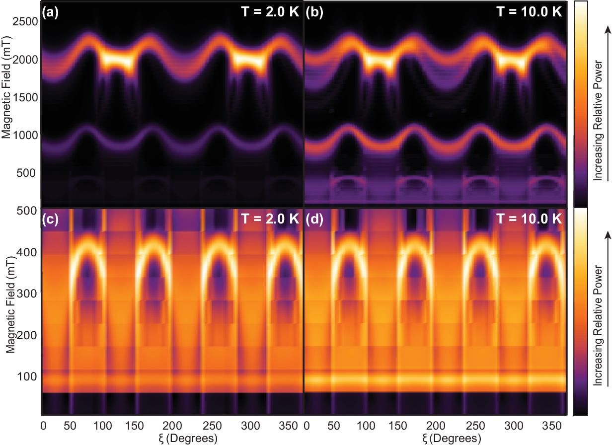
We measured cw ESR field spectra at intervals in of 4.5∘, resulting in 81 spectra being taken over a full rotation. The resonant frequency of the LGR was 3.78 GHz. Figure 6 shows the change in reflected power as a function of field over a full range in , at both T = 2.0 K (panels (a) and (c)) and T = 10.0 K (panels (b) and (d)). Near 2000 mT, transition peaks represent the ground state tunnel-split transition (), while the transitions near 1000 mT are the transition. The and transitions each have two expected peaks for the two comformational states of Ni4, but they lie very close together and cannot be clearly resolved. At low fields, visible in panels (a) and (b), as well as in further detail in panels (c) and (d), are the peaks of the transition (the transition also appears faintly at mT). The lower panels use a different color scale for clarity. For certain values of , there are two clear peaks visible in the 200 – 400 mT range, corresponding to the bifurcation of the transition. As is rotated through a full circle, the fourfold nature of the bifurcation appears clearly: As is varied, the two peaks become closer together and eventually merge into one, behaving qualitatively as expected (cf. Fig. 3).
In Fig. 6, the highly visible ( mT) and ( mT) transitions reveal two obvious patterns. The peak positions of both transitions shift as is varied, as expected when the transverse field sweeps through the hard plane of Ni4. In addition, the amplitude of the transitions changes dramatically. This is due to the crystal misalignment (Fig. 5(b)). When the crystal easy (z) axis is in the X-Y plane, the DC field lies in the hard plane and the pairs of states can be well approximated by the superposition states , with a large radiative coupling within each pair. However, as the sample is rotated, the easy axis leaves the X-Y plane, resulting in a small component of the DC field along the easy axis, , that tends to localize the eigenstates, reducing the transition matrix elements between the two states so the transitions are suppressed.sup This effect is less pronounced at low fields since a small DC field results in a correspondingly small when the sample is rotated out of the X-Y plane.
Superimposed on the data in Fig. 6 are curves corresponding to the theoretically predicted positions of the transitions. Due to the closeness of the peaks of each conformational state in the Ni4 SMM, the theoretical curves for the and transitions show the average predicted position of the peak positions. In contrast, for the transition, theory predicts rather different results from the two conformational states and so the curves for both conformation states are presented. Fig. 6 illustrates our fundamental finding: the periodic bifurcation of the transition (panels (c,d)), as predicted (Fig. 3) due to the Berry phase interference and the existence of a diabolical point in this pair of levels. The fact that the observed positions of the resonances agree with the theoretical predictions lends strong credence to this interpretation. The figure also demonstrates the four-fold symmetry of the peak positions, especially in the lower panels, with the pattern repeating every 90∘. Also apparent, especially in the upper panels, is the effect of misalignment, which produces much stronger signals at two values of 180∘ apart, corresponding to the orientations when the sample’s easy axis lies in the X-Y plane and . Since the transition corresponds to a transition between high-lying levels (cf. Fig. 1), these transitions become stronger at higher temperatures, as shown in the right panels of Fig. 6. Similarly, the transition is stronger at higher temperature while the transition, a ground-state transition, becomes weaker as the temperature is increased.


III.1 Simulations and Fitting
Simulated spectra were produced using the EasySpin package for Matlab.Stoll and Schweiger 2006 We used simulated spectra to fit our data using a least-squares method and extract relevant parameters (discussed below). To reasonably reproduce our experimental spectra, we needed to account for various factors, including misalignment and the effects of dipole fields within the sample. These factors have correlated effects, requiring them to be treated carefully.
To start, we take into account that the field seen by a typical spin in the sample differs from the applied field :
| (3) |
for the th Cartesian component, where characterizes lattice and demagnetization effects.Chen et al. 2016 The magnetization has both a mean value and a small random portion :
| (4) |
The former can be determined using basic statistical mechanical techniques:
| (5) |
where is the unit cell volume of Ni4. The matrix elements and energies are found by diagonalizing the spin Hamiltonian (Eq. 1) for each conformational state to calculate the magnetization for that state. The net magnetization is obtained by taking the average of the magnetizations of the two conformation states. Hamiltonian parameters used for the calculations are based on previously determined values.Chen et al. 2016
The random field is due to fluctuations of about equilibrium and arises from the configuration of neighboring spins. Since the molecule is an easy-axis system, we assume the primary direction for the random dipole fields is the z axis and neglect the other components: . is assumed to have a Gaussian-weighted distribution of width :
| (6) |
Calculation of a spectrum proceeds as follows. For a given applied field , and orientation of the crystal (specified by angles , , and ), the components along the crystal axes are calculated. Given a temperature , for each value of in a distribution of width , we numerically invert Eq. 3, making use of Eq. 4, to determine the components of , the field experienced by a spin. Using a range of values , the total (weighted) spectral response is then calculated for this field and the procedure is iterated over the full range of to obtain a complete spectrum. In addition, the effects of strain can be included in the calculated spectrum. These effects are essentially indistinguishable from those of crystal mosaicicity, as discussed below. Iteration of this procedure over every value of creates a simulation of the full experiment.
III.2 Fitting Results
We implemented a least-squares fitting routine that considered the full behavior of the spectrum at every measured value of . Fitting includes only the and transitions since the other observed transitions are too small to have a significant effect on the fits. The results of fitting are shown in Fig. 7, and partially in Fig. 8. The fits reasonably reproduce the experimental results, although the amplitude of the peaks vary as a function of more in the actual data than in the fitted spectra, as shown in Fig. 8. While we do not have a definitive explanation for this discrepancy, we conjecture that it may result from sample heating by the radiation, as discussed further below. Nevertheless, the peak positions agree very well. Remarkably, although the low-field data was not included in the fitting routine, the simulated spectra reproduce the observed interference effects in the transitions extremely well (cf. Fig. 6 and Fig. 7(c,d)). This provides strong confirmation that we are observing the anticipated Berry phase interference in Ni4.
Fitting parameters include the misalignment angle ; initial orientations of the crystal and apparatus, and respectively; the dipole Gaussian width ; the magnetization factor ; strain; and the temperature; as well as an overall scaling factor. We fit data taken at both 2 K and 10 K. Since the same sample was measured at both temperatures in a single cool down, the difference is the same for both sets of data. We treat as the free parameter that, with the value of for each temperature, determines the value of for that temperature. Best-fit values of these parameters are given in Table 1. Parameters , and strain represent intrinsic properties of the sample while is an essential property of the experiment. In contrast, , and are “accidental” properties relating the sample or apparatus alignment. For completeness, the table also includes a value for a mosaic distribution width that produces spectra (and therefore a fit) that is essentially identical to that obtained with the given value of strain. We treat the mosaicicity as a Gaussian distribution in angular orientations of individual molecules within the crystal, where the center of the Gaussian represents the overall orientation of the crystal itself. (Use of strain for fitting is computationally more efficient.)
The value of obtained from the fitting is on the order of the nearest-neighbor dipole field for molecules in the crystal. The fitted value of agrees with the value determined in previous experiments on Ni4.Chen et al. 2016 While a strain on the order of 12% is surprisingly large, it translates into a mosaic spread of that is reasonable for molecular crystals.
| Parameter | Value |
|---|---|
| 14(3) mT | |
| 4(1) | |
| T (2.0 K data) | 3.9(6) K |
| T (10.0 K data) | 12.7(6) K |
| (2.0 K data) | |
| (10.0 K data) | |
| strain | 12(4)% |
The most significant deviations of fitting parameters from experiment are in the fitted temperatures, as mentioned above. For the 2.0 K data, the fit temperature is 3.9 K, nearly twice the experimental temperature. This may indicate an issue of sample heating by the applied microwave radiation. Indeed, these experiments were done at high power (0 dBm) to obtain a good signal-to-noise ratio. Heating by absorption of radiation (and emission of phonons) drives the system out of thermal equilibriumBal et al. 2004; Bal et al. 2005 and depends on the transition: more heating is expected for the ground-state transition. Thus, use of a “temperature” for a spectrum (or set of spectra) is heuristic and does not fully characterize the level populations of the system as a function of field. In keeping with this interpretation, we find that for the 10.0-K data, the fit temperature of 12.7 K is a significantly smaller relative deviation, as one might expect: when the temperature is higher, the sample has a higher specific heat and better effective thermal coupling to the cryostat reservoir. The amount of heating may further depend on because of changes in the matrix element as the sample’s easy axis is rotated in and out of the X-Y plane, resulting in temperature changes that cannot be accounted for with a single value of temperature for a full set of data. This may account for the disagreement between experimental and simulated peak amplitudes seen in Fig. 8.
IV Conclusion
In this paper we have provided compelling evidence of Berry phase interference effects in the single-molecule magnet Ni4. In particular, we explored an excited-state tunneling transition that shows a bifurcation at a given frequency as the applied magnetic field is swept. This doubling is dependent on the angle of the applied field relative to the hard axes of the crystal, and as such, modulation of these transitions occurred as the crystal was rotated. An in situ method of sample rotation allowed investigation of the behavior as the field direction is swept through the hard plane of the sample, and showed the expected periodic bifurcation of the resonances, the hallmark of Berry phase interference.
Furthermore, simulations of the ESR spectra clearly reproduce the bifurcation effects and show agreement with data from other excited transitions. We found that sample misalignment and the effects of dipolar interactions between molecules in the crystal to be a significant factors that needed to be incorporated in the simulations to adequately reproduce the experimental spectra.
Acknowledgements.
We thank G. Joshi and K. Jagannathan for useful conversations and advice, A. Anderson for assistance with use of the computing cluster, J. Kubasek for assistance with design and machining of the rotation apparatus, and R. Winn for 3D printing of portions of the apparatus. Support for this work was provided by the U.S. National Science Foundation under Grant Nos. DMR-1310135 and DMR-1708692, and by the Amherst College Dean of Faculty. J.R.F. acknowledges the support of the Amherst College Senior Sabbatical Fellowship Program, funded in part by the H. Axel Schupf ’57 Fund for Intellectual Life. R.A.A. Cassaro thanks FAPERJ and CNPq for financial support. T.A. Costa acknowledges CNPq for the fellowship.References
- Friedman and Sarachik (2010) J. R. Friedman and M. P. Sarachik, Annu. Rev. Condens. Matter Phys. 1, 109 (2010).
- Garg (1993) A. Garg, Europhys. Lett. 22, 205 (1993).
- Park and Garg (2002) C.-S. Park and A. Garg, Phys. Rev. B 65, 064411 (2002).
- Kim (2002) G.-H. Kim, J. Appl. Phys. 91, 3289 (2002).
- Foss-Feig and Friedman (2009) M. S. Foss-Feig and J. R. Friedman, Europhys. Lett. 86, 27002 (2009).
- Wernsdorfer and Sessoli (1999) W. Wernsdorfer and R. Sessoli, Science 284, 133 (1999).
- Wernsdorfer et al. (2002) W. Wernsdorfer, M. Soler, G. Christou, and D. N. Hendrickson, J. Appl. Phys. 91, 7164 (2002).
- Lecren et al. (2005) L. Lecren, W. Wernsdorfer, Y.-G. Li, O. Roubeau, H. Miyasaka, and R. Clérac, J. Am. Chem. Soc. 127, 11311 (2005).
- Adams et al. (2013) S. T. Adams, E. H. da Silva Neto, S. Datta, J. F. Ware, C. Lampropoulos, G. Christou, Y. Myaesoedov, E. Zeldov, and J. R. Friedman, Phys. Rev. Lett. 110, 087205 (2013).
- Wernsdorfer et al. (2005) W. Wernsdorfer, N. E. Chakov, and G. Christou, Phys. Rev. Lett. 95, 037203 (2005).
- Atkinson et al. (2014) J. H. Atkinson, R. Inglis, E. del Barco, and E. K. Brechin, Phys. Rev. Lett. 113, 087201 (2014).
- Waldmann et al. (2009) O. Waldmann, T. C. Stamatatos, G. Christou, H. U. Güdel, I. Sheikin, and H. Mutka, Phys. Rev. Lett. 102, 157202 (2009).
- del Barco et al. (2004) E. del Barco, A. D. Kent, E. C. Yang, and D. N. Hendrickson, Phys. Rev. Lett. 93, 157202 (2004).
- Leuenberger and Mucciolo (2006) M. N. Leuenberger and E. R. Mucciolo, Phys. Rev. Lett. 97, 126601 (2006).
- Wernsdorfer et al. (2008) W. Wernsdorfer, T. C. Stamatatos, and G. Christou, Phys. Rev. Lett. 101, 237204 (2008).
- Quddusi et al. (2011) H. M. Quddusi, J. Liu, S. Singh, K. J. Heroux, E. del Barco, S. Hill, and D. N. Hendrickson, Phys. Rev. Lett. 106, 227201 (2011).
- Yang et al. (2003) E.-C. Yang, W. Wernsdorfer, S. Hill, R. S. Edwards, M. Nakano, S. Maccagnano, L. N. Zakharov, A. L. Rheingold, G. Christou, and D. N. Hendrickson, Polyhedron 22, 1727 (2003).
- Lawrence et al. (2008) J. Lawrence, E.-C. Yang, R. Edwards, M. M. Olmstead, C. Ramsey, N. S. Dalal, P. K. Gantzel, S. Hill, and D. N. Hendrickson, Inorg. Chem. 47, 1965 (2008).
- (19) See supplemental material at [URL will be inserted], for details on data acquisition, analysis and calculations.
- Yang et al. (2006) E.-C. Yang, W. Wernsdorfer, L. N. Zakharov, Y. Karaki, A. Yamaguchi, R. M. Isidro, G.-D. Lu, S. A. Wilson, A. L. Rheingold, H. Ishimoto, and D. N. Hendrickson, Inorg. Chem. 45, 529 (2006).
- Collett et al. (2016) C. A. Collett, R. A. A. Cassaro, and J. R. Friedman, Phys. Rev. B 94, 220402 (2016).
- Stoll and Schweiger (2006) S. Stoll and A. Schweiger, Journal of Magnetic Resonance 178, 42 (2006).
- Chen et al. (2016) Y. Chen, M. D. Ashkezari, C. A. Collett, R. A. A. Cassaro, F. Troiani, P. M. Lahti, and J. R. Friedman, Phys. Rev. Lett. 117, 187202 (2016).
- Bal et al. (2004) M. Bal, J. R. Friedman, Y. Suzuki, K. M. Mertes, E. M. Rumberger, D. N. Hendrickson, Y. Myasoedov, H. Shtrikman, N. Avraham, and E. Zeldov, Phys. Rev. B 70, 100408 (2004).
- Bal et al. (2005) M. Bal, J. R. Friedman, Y. Suzuki, E. M. Rumberger, D. N. Hendrickson, N. Avraham, Y. Myasoedov, H. Shtrikman, and E. Zeldov, Europhys. Lett. 71, 110 (2005).