A frequency-dependent -adaptive technique for spectral methods
Abstract
When using spectral methods, a question arises as how to determine the expansion order, especially for time-dependent problems in which emerging oscillations may require adjusting the expansion order. In this paper, we propose a frequency-dependent -adaptive technique that adaptively adjusts the expansion order based on a frequency indicator. Using this -adaptive technique, combined with recently proposed scaling and moving techniques, we are able to devise an adaptive spectral method in unbounded domains that can capture and handle diffusion, advection, and oscillations. As an application, we use this adaptive spectral method to numerically solve the Schrödinger equation in the whole domain and successfully capture the solution’s oscillatory behavior at infinity.
Keywords:
unbounded domain, spectral method, adaptive method, Schrödinger equation, Jacobi polynomial, Hermite function, Laguerre function1 Introduction
Unbounded domain problems arise in many scientific applications [1, 2] and adaptive numerical methods are needed on many occasions, for instance, in solving the Schrödinger equation in unbounded domains when the solution’s behavior varies over time and we wish to capture the solution’s behavior in the whole domain. As an important class of numerical algorithms, adaptive methods have witnessed numerous advances in their efficiency and accuracy [3, 4, 5, 6]. However, despite considerable progress that has been made for spectral methods in unbounded domains [7], there are few adaptive methods that apply in unbounded domains.
In [8], adaptive scaling and moving techniques were proposed for spectral methods in unbounded domains and it was noted that adjusting the expansion order is necessary when the function displays oscillatory behavior that varies over time. In this paper, we first develop a frequency-dependent technique for spectral methods which adjusts the expansion order ( basis functions are used to approximate the solution). This technique takes advantage of the frequency indicator defined in [8] and corresponds to -adaptivity [9, 10, 11]. By adjusting the expansion order efficiently, our -adaptive technique can be used to accurately solve problems with varying oscillatory.
By combining this -adaptive technique with scaling and moving methods, we develop an adaptive spectral method that can capture diffusion, advection, and oscillations in unbounded domains. Since scaling and adjusting the expansion order both depend on the frequency indicator, we also investigate the interdependence of these two techniques. We demonstrate that appropriately adjusting the expansion order can facilitate scaling to more efficiently distribute allocation points. In turn, proper scaling can help avoid unnecessary increases in the expansion order when it does not increase accuracy, thereby avoiding unnecessary computational burden.
The significance of this adaptive spectral method is that it can capture the solution’s behavior in the whole domain. We demonstrate the utility of our method by solving Schrödinger’s equation in . Here, the unboundedness and the oscillatory nature of the solution pose two major numerical challenges [12]. Specifically, in the semiclassical regime, when the wavelength of the solution is small, the function becomes extremely oscillatory. Moreover, in certain situations, one has to work with a very large computational domain that is difficult to automatically determine.
Previous numerical methods which solve Schrödinger’s equation in unbounded domains usually truncate the domain into a finite subdomain and impose artificial boundary conditions, which may be nonlocal and complicated [13, 12, 14, 15]. Our adaptive spectral method tackles the oscillatory problem directly in the original unbounded domain without the need to truncate it or to devise an artificial boundary condition.
This paper is organized as follows. In the next section, we first present a -adaptive technique for spectral methods and use examples to illustrate its efficiency. In Section 3, we incorporate and study this technique within existing scaling and moving techniques and devise an adaptive spectral method in unbounded domains. Application of our adaptive spectral methods to numerically solving Schrödinger’s equation is given in Section 4. We summarize our results in Section 5 and propose directions for future work.
2 Frequency-dependent -adaptivity
We present a frequency-dependent -adaptive spectral method based on information extracted from only the numerical solution of time-dependent problems. In [8], we showed that a frequency indicator defined for spectral methods is particularly useful in measuring the contribution of high frequency modes in the numerical solution. Because high frequency modes decay more slowly, this indicator could be used to determine scaling in spectral methods applied to unbounded domains. In this work, we will show that the frequency indicator can also be used to determine whether more or fewer basis functions are needed to refine or coarsen the numerical solution.
Given a set of orthogonal basis functions under a specific weight function in a domain , the frequency indicator associated with the interpolation of a function
| (2.1) |
is defined as in [8]
| (2.2) |
where is the square of -weighted norm of the basis function . This frequency indicator measures the contribution of the highest-frequency components to the -weighted norm of . Here is often chosen to be following the -rule [16, 17]. This indicator provides a lower bound for the error divided by the norm of the numerical solution which is illustrated in [8]. Thus, the quality of the numerical interpolation can be measured by .
For a time-dependent problem, the expansion order may need adjusting dynamically, which can be reflected by the frequency indicator. If the frequency indicator increases, the lower bound for will also increase. On the other hand, as increases, the error as well as are expected to decrease. By sufficiently increasing the expansion order , the frequency indicator as well as the error can be kept small. If the frequency indicator decreases, we can also consider decreasing to relieve computational cost without compromising accuracy, as was done in [9]. The pseudo-code of the proposed -adaptive technique is given in Alg. 1.
The -adaptive spectral method in Alg. 1 for time-dependent problems consists of two ingredients: refinement (increasing ) and coarsening (decreasing ). It maintains accuracy when there are emerging oscillations by increasing the expansion order . It also decreases when the expansion order is larger than needed to avoid unnecessary computation. In Alg. 1, the frequency_indicator subroutine is to calculate the frequency indicator defined in Eq. (2.2) for the numerical solution while the evolve subroutine is to obtain the numerical solution at the next timestep from .
In Line 11 of Alg. 1, the refine subroutine uses to generate a new numerical solution with a larger expansion order (refine), and in Line 20 the coarsen subroutine uses to generate a new numerical solution with a smaller expansion order (coarsen). The refinement or coarsening is achieved by reconstructing the function values of or at the new set of collocation points :
| (2.3) |
where uses basis functions for refinement and uses basis functions for coarsening.
In Alg. 1, is the refinement threshold such that if the current frequency indicator , we increase the expansion order . The while loop starting in Line 9 ensures we either refine enough such that the frequency indicator, after increasing , is smaller than the threshold , or the maximal allowable expansion order increment within a single step is reached.
After increasing , is renewed to be the current frequency indicator and is multiplied by a factor , enabling us to dynamically adjust the refinement threshold for the next refinement in order to prevent increasing too fast without substantially increasing accuracy. On the other hand, when an extremely large is needed to match the increasingly oscillatory behavior of the numerical solution, we can set or even , as we will do in Examples 5 and 6. We have observed numerically, as expected, that the larger are, the more difficult it is to increase the expansion order.
We also consider reducing when a large expansion order is not really needed and is the threshold for decreasing the expansion order. If the condition in Line 17 is satisfied and , the minimal allowable expansion order, and we have not increased in the current step, on the contrary we consider decreasing the expansion order below Line 17. As long as the frequency indicator of the new numerical solution with the decreased expansion order is smaller than , the frequency indicator recorded after previously adjusting the expansion order, reducing the expansion order is accepted; else reducing the expansion order is declined. Therefore, after coarsening will not surpass before coarsening. This procedure is described by the If condition in Line 22. If is decreased, will also get renewed to be the latest frequency indicator.
In addition, if the current frequency indicator , neither the refinement nor the coarsening subroutine is activated.
Alg. 1 can be generalized to higher dimensions in a dimension-by-dimension manner. The expansion order for each dimension can change simultaneously within each timestep by using the tensor product of one-dimensional basis functions, in much the same way moving and scaling algorithms were generalized to higher dimensions [8]. For example, for a two-dimensional problem, given
| (2.4) |
where , the frequency indicator in the -direction is defined as
| (2.5) |
while the frequency indicator in -direction is similarly defined. At each timestep, we keep fixed and use to judge whether or not to renew ; simultaneously, we fix and use to renew if adjusting the expansion order in dimension is needed. Finally are updated to .
In this work, the relative -error
| (2.6) |
is used to measure the quality of the spectral approximation compared to the reference solution . Table 1 lists some typical choices of orthogonal basis functions for different domains that we use in this paper.
Computational domain Bounded interval Basis functions Jacobi polynomials Laguerre polynomials/functions Hermite polynomials/functions
We provide two examples of using this -adaptive technique in Alg. 1 below, where the generalized Jacobi polynomials [18] are used. Theorem 3.41 in [18] gives an estimation for the interpolation error of a function in the Jacobi-weighted Sobolev space for as follows
| (2.7) | ||||
where is a positive constant independent of and . When and , the left hand side becomes the interpolation error which decreases with . Therefore, by increasing the expansion order for the Jacobi polynomials it is generally true that the interpolation will be more accurate. Theorem 7.16 and Theorem 7.17 in [18] give similar error estimates for Laguerre and Hermite interpolations, which reveals that under some smoothness assumptions, the interpolation error decreases when the expansion order increases.
Since unbounded domain problems may involve diffusive and advective behavior, we discuss and develop adaptive spectral methods in unbounded domains in the next section.
Example 1
We numerically solve the PDE
| (2.8) |
with a Dirichlet boundary condition specified at given as . This PDE admits an analytical solution
| (2.9) |
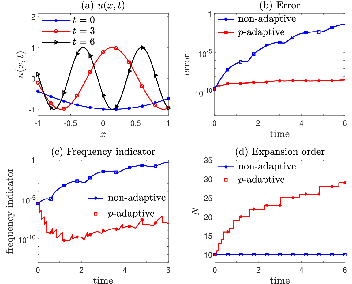
We solve it numerically by using Chebyshev polynomials with Chebyshev-Gauss-Robatto quadrature nodes and weights. The Chebyshev polynomials are orthogonal under the weight function , i.e., they correspond to Jacobi polynomials with . Since becomes increasingly oscillatory over time, an increasing expansion order is required to capture these oscillations. We start with at , the parameters , and a timestep . We use a third order explicit Runge-Kutta scheme to advance time.
The reference solution is plotted in Fig. 1(a). The increasing oscillations lead to a fast rise in the frequency indicator as the contribution from high frequency modes increases. Keeping the same number of basis functions over time will fail as it will be eventually incapable of capturing the shorter wavelength oscillations.
However, a much more accurate approximation can be obtained (see Fig. 1(b)) with our -adaptive method which maintains the frequency indicator (see Fig. 1(c)) by increasing the number of basis functions (shown in Fig. 1(d)). Furthermore, the coarsening subroutine for decreasing the expansion order described in the while loop in Line 17 will not be triggered (shown in Fig. 1(d)).
When directly approximating the reference solution in Eq. (2.9), we can achieve accuracy with only 20 basis functions. However, when numerically solving Eq. (2.8), the error will accumulate due to the increasing oscillatory behavior which will require even more basis functions to achieve the same accuracy as the direct approximation to Eq. (2.9). Thus, the oscillatory behavior of the solution poses additional difficulties and requires even more refinement when numerically solving a PDE.
Next, we present an example of a two-dimensional problem in .
Example 2
We approximate the function
| (2.10) |
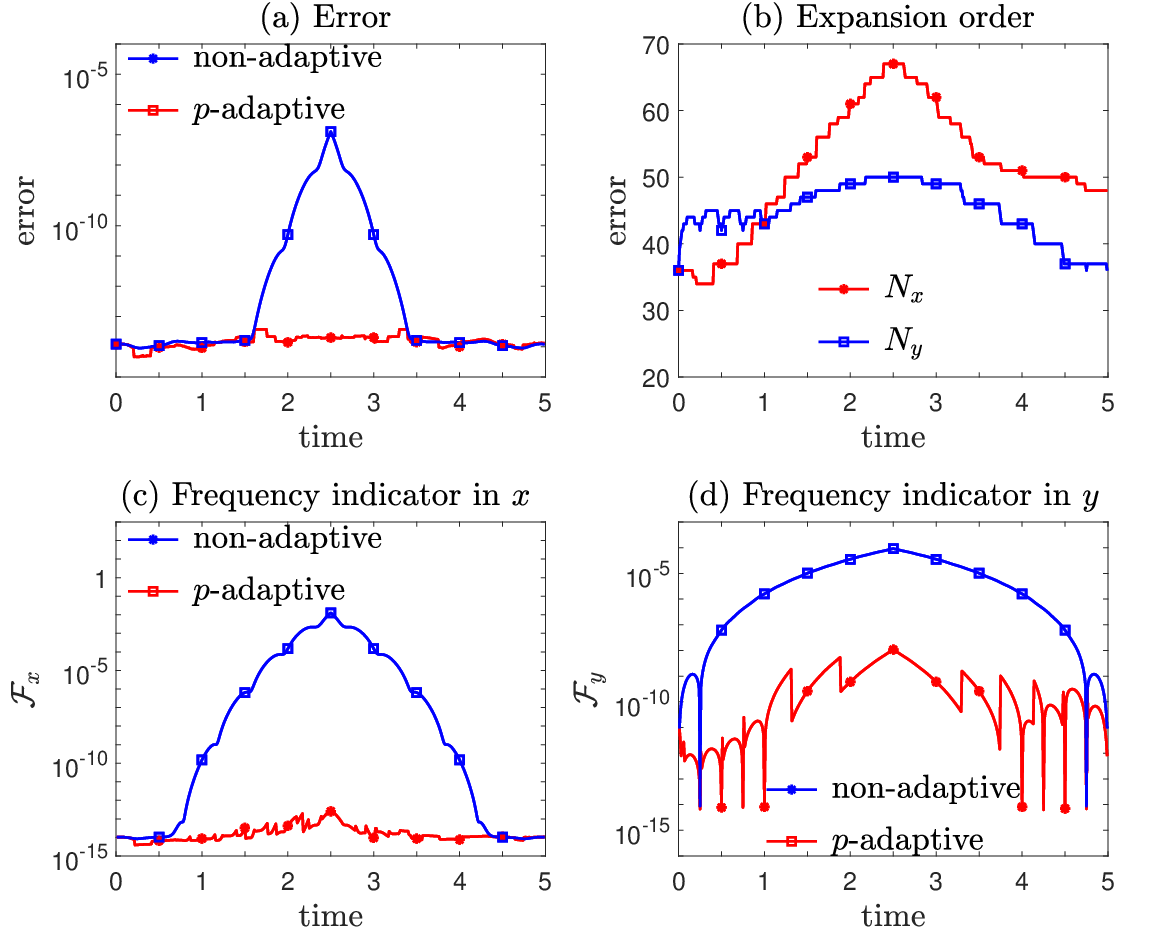
by Legendre polynomials (corresponding to Jacobi polynomials with ) with Legendre-Gauss-Robatto quadrature nodes and weights in both dimensions. Within , the function becomes more oscillatory over time in both dimensions, requiring increasing expansion orders. For , the error for approximation with fixed expansion orders in both dimensions decreases because the function becomes less oscillatory, and therefore a reduction in expansion orders in both directions can be used to reduce computational effort without compromising accuracy. Since the function is not symmetric in and and the adjustment of expansion is anisotropic. We show that Alg. 1 can appropriately increase when and reduce when . We take at with a timestep , and .
It is clear from Fig. 2(a) that fixing the number of basis functions in each dimension leads to an approximation which deteriorates while the proposed -adaptive spectral method is able to keep the error small. Furthermore, when we see that with fixed expansion order the approximation error decreases, indicating that coarsening may be performed to relieve computational burden while maintaining accuracy. Alg. 1 first tracks the increasing oscillation by increasing expansion orders in both and dimensions. When , Alg. 1 senses a decrease in frequency indicator and decreases both and adaptively (shown in Figs. 2(b)) without compromising accuracy, as shown in Fig. 2(a).
Since is the most oscillatory term in , the function becomes more oscillatory in than in when . Because the function displays different oscillatory behavior in - and -directions, the expansion order should be adjusted anisotropically and needs increasing more than in order to maintain small. Both and are maintained well for the -adaptive approximation over time (shown in Fig. 2(c) and (d)), leading to satisfactory error control. Overall, Alg. 1 preserves accuracy for all times while still avoids using excessive values of and when they are not needed.
3 Adaptive spectral methods in unbounded domains
Unbounded domain problems are often more difficult to numerically solve than bounded domain problems. Diffusion and advection in unbounded domains necessitates knowledge of the solution’s behavior at infinity. To distinguish and handle diffusive and advective behavior in unbounded domains, techniques for scaling and moving basis functions are proposed in [8]. When combining scaling, moving, refinement and coarsening, we can devise a comprehensive adaptive spectral approach for unbounded domains. A flow chart of our overall approach is given in Fig. 3. The scaling, refinement and coarsening techniques all rely on a common frequency indicator.
As is stated in [8], advection may cause a false increase in the frequency indicator. Thus, we must first compensate for advection by the moving technique before we consider either scaling or adjusting the expansion order. Next, as the cost of changing the scaling factor is lower than increasing the expansion order, we implement scaling before adjusting the expansion order. Only if scaling cannot maintain the frequency indicator below the refinement threshold do we consider increasing the expansion order. Coarsening is also considered after scaling if the frequency indicator decreases below the threshold for coarsening while no refinement is performed in the current timestep.
As we have done in [8], we also decrease the scaling factor by multiplying it by a common ratio if the current frequency indicator is larger than the scaling threshold . The scaling we perform here contains an additional step: when the current frequency indicator decreases and is below , we consider increasing the scaling factor by dividing it by the common ratio as long as the frequency indicator decreases after increasing . When , is neither increased nor decreased. Thus, at each step, the scaling factor may be either increased or decreased as long as the frequency indicator decreases after adjusting the scaling factor. A decrease in the scaling factor indicates that the allocation points are more efficiently distributed. These changes avoid unnecessary computational burden that may arise if is excessively increased. We briefly describe our modified scaling subroutine for one timestep in Alg. 2.
For simplicity, we assume that the function is moving rightward so we need to move the basis functions rightward. Therefore, is the “exterior domain" of the spectral approximation on which we wish to control the error as illustrated in [8]. For Laguerre polynomials/functions the parameter in the algorithm in Fig. 3 denotes the starting point for the approximation, while for Hermite polynomials/functions represents the translation of Hermite polynomials/functions, i.e., we use or . After the expansion order has changed, we need to renew both the threshold for scaling and the threshold for adjusting the expansion order. We also need to renew the threshold for moving, denoted by , after has changed because different leads to different . is the spectral approximation with the scaling factor . Here the exterior-error indicator for the semi-unbounded domain is defined in [8] and we can generalize it to when using Hermite polynomials/functions
| (3.1) |
where is the weight function and is taken to be for Hermite functions/polynomials and for Laguerre functions/polynomials [8] in view of the often-used -rule. The difference between the choices of for Hermite and Laguerre basis functions arises because the allocation points for Hermite functions are symmetrically distributed around their center while those for Laguerre functions are one-sided, to the right of the starting point in the axis.
For the scaling subroutine we need the following parameters: the common ratio that we use to geometrically shrink/increase the scaling factor, the parameter describing the threshold for considering shrinking the scaling factor ; a predetermined lower bound for the scaling factor and an upper bound . For the moving subroutine, required parameters include the minimal displacement for the moving technique , the maximal displacement within a single timestep , and the parameter of the threshold for activating the moving technique . The scale and move in Fig. 3 are the scaling and moving subroutines and exterior_error_indicator calculates the exterior-error indicator for the moving subroutine. Detailed discussions about scaling and moving techniques are given in [8].
After first applying the moving technique, adjusting the expansion order and scaling both depend on the frequency indicator and aim to keep the frequency indicator low to control the error. The relationship and interdependence between them is key to understanding and justifying the first-scaling-then-adjusting expansion-order procedure in Fig. 3. Thus, we need to investigate how the proposed scaling technique will affect our -adaptive technique and how these two techniques interact with each other. We use two examples containing both diffusive and oscillatory behavior to investigate how the two techniques will be activated and influence each other. In Example 3, both refinement and reducing are needed for matching increasing oscillatory and diffusive behavior of the solution; in Example 4, a less oscillatory and diffusive solution over time implies that coarsening and increasing may be considered.
1.2 1.5 2 4 1.05 1.1 1.2 1.5
Example 3
We approximate the function
| (3.2) |
with the generalized Laguerre function basis discussed in [8] with the parameter . The magnitude of oscillations for this function, , increases over time, requiring proper scaling. Under a variable transformation , can be rewritten as , indicating that the solution is increasingly oscillatory in as time increases. Thus, if we reduce the scaling factor to match the diffusive behavior of the solution, proper refinement is also required. In other words, diffusive and oscillatory behavior is coupled in this example. We carry out numerical experiments using the algorithm described in Fig. 3 with different to investigate how scaling and refinement influence each other. We deactivate the moving technique by setting since the solution exhibits no intrinsic advection. Even if we had allowed moving, it was hardly activated. We set at and . and choose the initial scaling factor .
1.2 1.5 2 4 1.05 1.1 1.2 1.5
In Table 2 and Table 3 the error in is recorded in the lower-left part of each entry while the scaling factor and expansion order at is recorded in the upper-right. By comparing entries in each column/row for smaller , both tables show the expansion order is likely to be increased more when the threshold for refinement is lower.
It can be observed from Table 2 that with more refinement tends to be smaller. This interaction between -adaptivity and scaling arises because more refinement leads to a larger expansion order and a smaller scaling threshold . Since scaling will only be performed if the frequency indicator after scaling decreases, proper refinement is not likely to lead to over-scaling.
Moreover, by comparing at between Tables 2 and 3, we see that tends to be smaller with the scaling technique for the same . This implies that without scaling, the refinement procedure is more often activated, leading to a larger to compensate for the incapability of scaling alone to maintain a low frequency indicator. This results in a larger computational burden without an improvement in accuracy. This behavior has been expected from the design of Alg. 3 since we put scaling before refinement so that redistribution of collocation points is tried first to avoid unnecessary refinement when the increase in frequency indicator results from diffusion instead of oscillation.
Example 4
We approximate the function
| (3.3) |
with the generalized Laguerre function basis with the parameter . The magnitude of oscillations for this function, , decreases over time and increasing the scaling factor to more densely redistribute the allocation points is needed. Furthermore, under the variable transformation , can be rewritten as . Since the oscillations decrease with , one can reduce the expansion order. We consider coarsening with or without scaling to investigate whether increasing can facilitate coarsening (and save computational effort) or result in higher accuracy. We carry out numerical experiments using the algorithm described in Fig. 3 and different and also deactivate the moving technique by setting since the solution exhibits no intrinsic advection. We set at the beginning and set the parameters , and initial scaling factor . We use a different threshold for coarsening and we have checked numerically that the parameter in the refinement subroutine will not affect the coarsening subroutine in this example.
1.2 1.5 2 4 Scaled Unscaled
In Table 4 the error in is recorded in the lower-left part of each entry while the scaling factor and expansion order at is recorded in the upper-right. By comparing entries in each row we see that a smaller will lead to easier coarsening and a smaller at . Since the approximation with larger is always better, whether we can achieve the same level of accuracy with a smaller expansion order if proper scaling is implemented is of interest. The initial approximation error is and the approximation will not worsen after coarsening regardless of because in the -adaptive subroutine coarsening is allowed only when the post-coarsening frequency indicator remains below the previous threshold . Moreover, by comparing the two rows in Table 4 we see that if the solution concentrates and becomes less diffusive, increasing and more efficiently redistributing the allocation points allows the scaling technique to achieve high accuracy with fewer expansion orders than without the scaling technique.
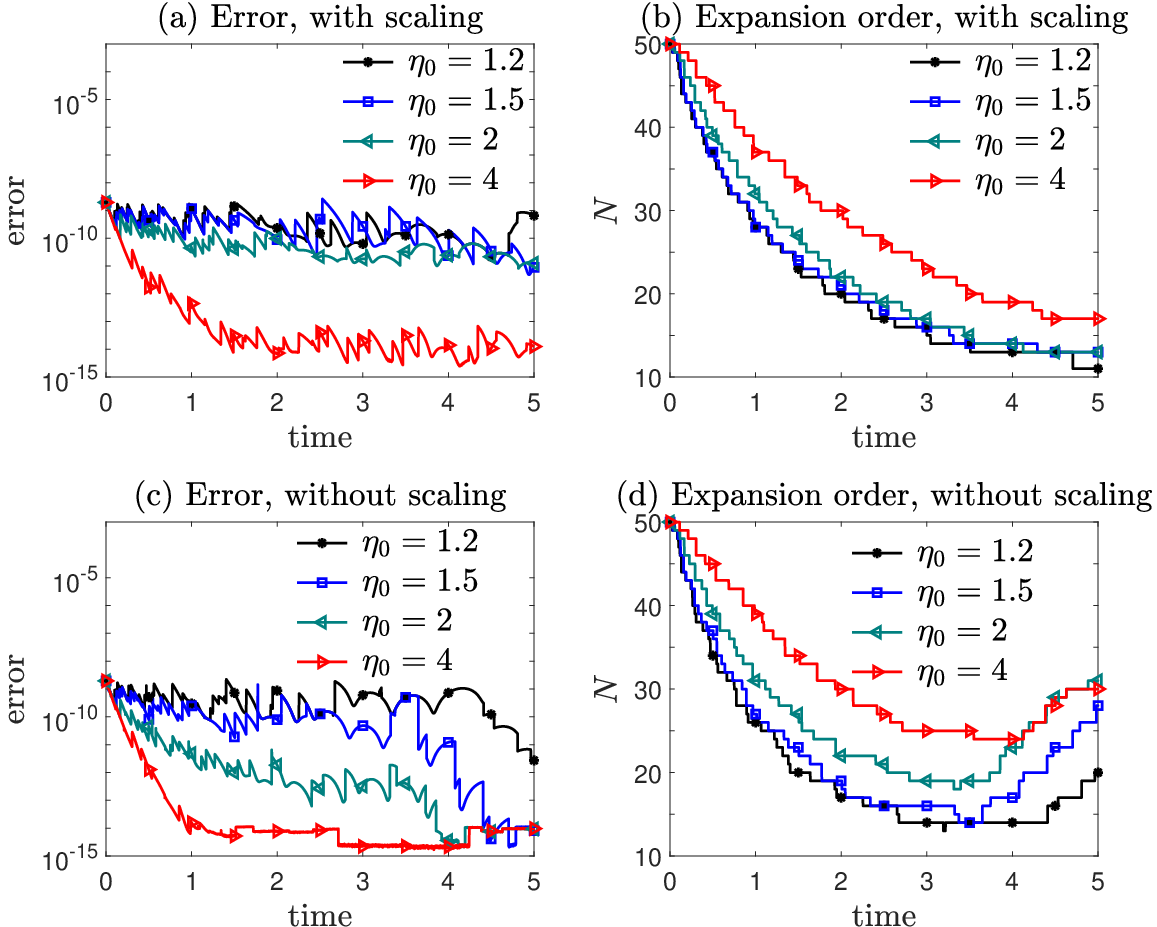

The errors and expansion orders over time are plotted in Fig. 4 where the -adaptive method is compared with the non--adaptive method when scaling is applied. From Figs. 4(a) and (c) we can observe that both scaled and unscaled methods maintain the error below the initial approximation error. Yet, upon comparing Fig. 4(b) to Fig. 4(d) it is readily seen that the scaled method leads to appropriate coarsening while succeeding in maintaining low error, but the unscaled method will increase when increasing the expansion order is not actually needed, resulting in additional unnecessary computational burden. In Fig. 4(e) the scaled and -adaptive spectral method with is compared with the scaling-only spectral method. We see that the errors for both methods are almost the same but the -adaptive method can reduce unnecessary computation by decreasing adaptively while still maintaining a low error, and the approximation error for the -adaptive method fluctuates due to a decreasing .
Fig. 4(f) shows that the scaling factor is increased more in the -adaptive method, implying that the reason why the -adaptive method can achieve the same accuracy as non--adaptive method with a smaller expansion order is that it can redistribute the allocation points more efficiently.
Finally, we conclude that all three methods: scaling, -adaptive+scaling, and -adaptive methods can maintain the error well below the initial approximation error, but the combined -adaptive+scaling method can achieve this with the smallest expansion order and is therefore the most efficient method among them.
4 Applications in solving the Schrödinger equation
In this section, we apply our adaptive spectral methods described in Fig. 3 to solve the Schrödinger equation in unbounded domains
| (4.1) |
which is equivalent to the PDE discussed in [14]
| (4.2) |
under the transformation . Here, we shall use spectral methods with the Hermite function basis. The solution is complex, so in the spectral decomposition the coefficients of the basis functions are complex. The major difference here is that in [14] the Schrödinger equation is solved in a bounded domain with absorbing boundary conditions. Using spectral methods, we are able to solve the Schrödinger equation without truncating the domain.
| (4.4) |
We denote , which can be analytically solved to advance time
| (4.5) |
where is a symmetric matrix with entries
| (4.6) |
and the matrix has entries
| (4.7) |
The evaluation of is performed as follows. First, we denote where the integration is evaluated by Gauss-Legendre formula. Therefore, when calculating the matrix-vector product for a vector , its component is
| (4.8) | ||||
where . We can first calculate
| (4.9) |
for each subindex ; then, evaluating for each subindex will only require an operation. In this way, given any arbitrary potentials we can calculate in operations without explicitly calculating entries in . We approximate the matrix-vector product in the following way: we rewrite , which is introduced as the “scaling and squaring" method in [19], and approximate the matrix-vector product by truncating the infinite Taylor expansion series . Here, we take .
As mentioned in Section 1, two main numerical difficulties when solving the Schrödinger equation are the unboundedness and oscillatory behavior of the solutions. In fact, the solution may be increasingly oscillatory behavior at infinity over time, making it very hard to solve in the unbounded domain. However, with our adaptive spectral methods, we can efficiently solve the Schrödinger equation in unbounded domains accurately and capture these oscillations.
We shall revisit the two numerical examples discussed in [14]. In the following examples, curves labeled “adaptive” indicate that scaling, moving, and -adaptive techniques are all applied as in the algorithm described in Fig. 3, while curves labeled “-adaptive” mean that Alg. 1 is used without scaling or moving; similarly, curves labeled “scaling & -adaptive” are obtained when the -adaptive and scaling techniques are applied. Curves labeled “scaling & moving” or “scaling" correspond to applying the scaling and moving techniques or the scaling technique without the -adaptive subroutine. The “non-adaptive” curves are obtained when we do not apply any of the scaling, moving, or -adaptive techniques.
Example 5
We numerically solve the Schrödinger equation which is solved in Example 1 of [14] and take in Eq. (4.1), admitting the analytic solution
| (4.10) |
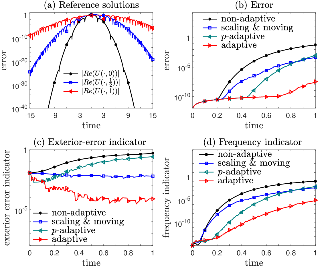
where is related to the propagation speed of the beam and determines the width of the beam. The absolute values of the real part of are plotted in Fig. 5(a), illustrating the increasingly oscillatory and diffusive behavior in the rightward propagating solution. Treatment of this solution will thus require scaling, moving, and -adaptive techniques. The imaginary parts of the reference solution (not plotted) over time are also increasingly oscillatory. We shall apply the algorithm described in Fig. 3. We set , and initialize at . Other parameters are set to , and . Note that with zero potential, Eq. (4.5) reduces to
| (4.11) |
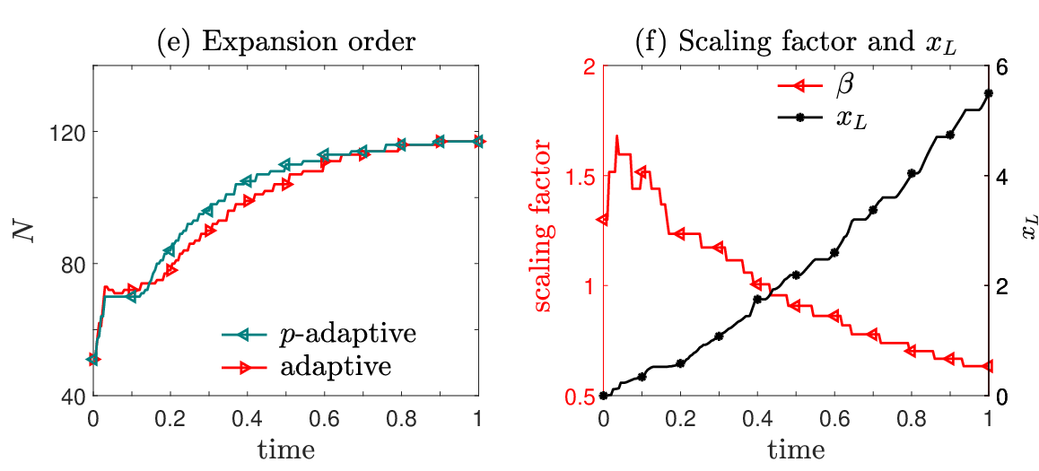
When all four techniques are applied, the error is the smallest (shown in Fig. 5(b)) since we can keep the exterior error indicator in small (shown in Fig. 5(c)) by matching the solution’s intrinsic advection. We can simultaneously prevent the frequency indicator from growing too fast (shown in Fig. 5(d)), thus ensuring a small error bound.
From the reference solution it can be observed that increasing the expansion order over time is an intrinsic requirement and failure to do so prevents the capture of the increasing oscillations, leading to a huge error. As the function becomes increasingly oscillatory as , moving the basis rightward requires correspondingly more refinement (shown in Fig. 5(e)). However, the -adaptive method alone cannot compensate for the inability to capture diffusion and advection, resulting in an inaccurate approximation. We have also checked that apart from what is shown in Fig. 5, applying any single scaling, moving or -adaptive technique, or combining any two of them will all result in a much larger error than employing all three techniques indicated in Fig. 3.
Finally, we numerically solve the Schrödinger equation with non-vanishing potentials.
Example 6
We numerically solve the following standard Schrödinger equation Eq. (4.1) equivalent to Example 2 in [14] with potentials
| (4.12) |
Given an even function as the initial condition for Example 2 in [14], the solution is also an even function and the solution of Eq. (4.1) obeys . No bias towards or is preferred. Therefore, we use the Hermite function basis and apply the algorithm described in Fig. 3 but deactivate the moving technique by setting .
We set the initial condition to be the same as that of Example 5 and set and at with the maximal expansion order increment for each step .
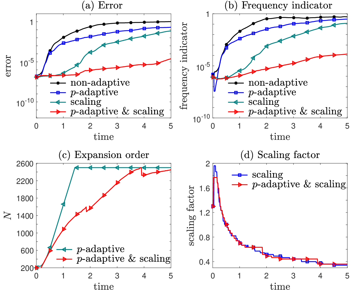
The reason why we set is that the expansion order needs to be increased quickly to catch up with the highly increasingly oscillatory behavior of the numerical solution. We set a uniform timestep . We use the numerical solution solved with a fixed and only the scaling technique activated as the reference solution. For the -adaptive method, we have added an additional restriction that the expansion order cannot surpass the expansion order of the reference solution .
We can easily see that the spectral method with both scaling and -adaptive techniques outperforms the non-adaptive spectral method or with only one of these two techniques employed (shown in Fig. 6(a)). The frequency indicator of using both scaling and -adaptive techniques is also the smallest (Fig. 6(b)), and the similarity between the frequency indicator and error is again confirmed as stated in [8]. Moreover, the unscaled method will result in a larger expansion order (shown in Fig. 6(a)), leading to excessive refinement with no improvement in accuracy (shown in Fig. 6(a)). In this example, the coarsening procedure will not lead to a large increase of frequency indicator and does not significantly compromise accuracy (shown in Figs. 6(b) and (c)). Finally, the scaling factors of the -adaptive spectral method and the non--adaptive spectral method trend similarly over time; they both decrease after experiencing an initial, transient increase (Fig. 6(d)).
5 Summary and Conclusion
In this paper, we proposed a frequency-dependent -adaptive technique that adjusts the expansion order for spectral methods. We demonstrated its applicability to time-dependent problems with varying oscillatory behavior. In order to develop efficient numerical methods for problems requiring solutions in unbounded domains, we also combined the -adaptive technique with scaling (-adaptivity) and moving (-adaptivity) methods to devise a complete adaptive spectral method that can successfully deal with diffusion, advection, and oscillation.
The relationship between scaling and -adaptive techniques for spectral methods in unbounded domains, both of which depend on the same frequency indicator, is also investigated. We successfully applied our adaptive spectral method to numerically solve Schrödinger’s equation. The associated solutions are highly oscillatory in the whole domain, posing numerical difficulties for existing numerical methods that truncate the domain.
For future research, the relationship among the adaptive techniques for spectral methods, scaling, moving, refinement and coarsening, can be further studied and rigorous numerical analysis for these techniques should be investigated. Furthermore, fast algorithms with mapped Chebyshev polynomials for solving PDEs in unbounded domains have been developed using the fast Fourier transform [20], but there lacks fast and efficient algorithms exploiting Laguerre and Hermite basis functions, particularly for higher-dimensional problems. Thus, generalizing these adaptive methods for mapped Jacobi polynomials may be a compelling future research direction.
Acknowledgments
MX and TC acknowledge support from the National Science Foundation through grant DMS-1814364 and the Army Research Office through grant W911NF-18-1-0345. SS acknowledges financial support from the National Natural Science Foundation of China (Nos. 11822102, 11421101) and Beijing Academy of Artificial Intelligence (BAAI). Computational resources were provided by the High-performance Computing Platform at Peking University.
References
- Tsynkov [1998] S. Tsynkov, Numerical solution of problems on unbounded domains. A review, Appl. Numer. Math. 27 (1998) 465–532.
- Xia et al. [2020] M. Xia, C. D. Greenman, T. Chou, PDE models of adder mechanisms in cellular proliferation, SIAM J. Appl. Math. 80 (2020) 1307–1335.
- Tang and Tang [2003] H. Tang, T. Tang, Adaptive mesh methods for one-and two-dimensional hyperbolic conservation laws, SIAM J. Numer. Anal. 41 (2003) 487–515.
- Babuska et al. [2012] I. Babuska, J. E. Flaherty, W. D. Henshaw, J. E. Hopcroft, J. E. Oliger, T. Tezduyar, Modeling, mesh generation, and adaptive numerical methods for partial differential equations, volume 75, Springer Science & Business Media, 2012.
- Ren and Wang [2000] W. Ren, X.-P. Wang, An iterative grid redistribution method for singular problems in multiple dimensions, J. Comput. Phys. 159 (2000) 246–273.
- Li et al. [2002] R. Li, W. Liu, H. Ma, T. Tang, Adaptive finite element approximation for distributed elliptic optimal control problems, SIAM J. Control Optim. 41 (2002) 1321–1349.
- Shen and Wang [2009] J. Shen, L. L. Wang, Some recent advances on spectral methods for unbounded domains, Commun. Comput. Phys. 5 (2009) 195–241.
- Xia et al. [2020] M. Xia, S. Shao, T. Chou, Efficient scaling and moving techniques for spectral methods in unbounded domains, submitted, arXiv:2009.13170 (2020).
- Shao et al. [2011] S. Shao, T. Lu, W. Cai, Adaptive conservative cell average spectral element methods for transient Wigner equation in quantum transport, Commun. Comput. Phys. 9 (2011) 711–739.
- Dumbser et al. [2007] M. Dumbser, M. Käser, E. F. Toro, An arbitrary high-order discontinuous Galerkin method for elastic waves on unstructured meshes-V. local time stepping and p-adaptivity, Geophys. J. Int. 171 (2007) 695–717.
- Karihaloo and Xiao [2001] B. L. Karihaloo, Q. Xiao, Accurate determination of the coefficients of elastic crack tip asymptotic field by a hybrid crack element with p-adaptivity, Eng. Fract. Mech. 68 (2001) 1609–1630.
- Yang and Zhang [2014] X. Yang, J. Zhang, Computation of the Schrödinger equation in the semiclassical regime on an unbounded domain, SIAM J. Numer. Anal. 52 (2014) 808–831.
- Han et al. [2005] H. Han, J. Jin, X. Wu, A finite-difference method for the one-dimensional time-dependent Schrödinger equation on unbounded domain, Comput. Math. Appl. 50 (2005) 1345–1362.
- Li et al. [2018] B. Li, J. Zhang, C. Zheng, Stability and error analysis for a second-order fast approximation of the one-dimensional Schrödinger equation under absorbing boundary conditions, SIAM J. Sci. Comput. 40 (2018) A4083–A4104.
- Antoine et al. [2008] X. Antoine, A. Arnold, C. Besse, M. Ehrhardt, A. Schädle, A review of transparent and artificial boundary conditions techniques for linear and nonlinear Schrödinger equations, Commun. Comput. Phys. 4 (2008) 729–796.
- Hou and Li [2007] T. Y. Hou, R. Li, Computing nearly singular solutions using pseudo-spectral methods, J. Comput. Phys. 226 (2007) 379–397.
- Orszag [1971] S. A. Orszag, On the elimination of aliasing in finite-difference schemes by filtering high-wavenumber components, J. Atmos. Sci. 28 (1971) 1074–1074.
- Shen et al. [2011] J. Shen, T. Tang, L. L. Wang, Spectral Methods: Algorithms, Analysis and Applications, Springer Science & Business Media, New York, 2011.
- Moler and Van Loan [1978] C. Moler, C. Van Loan, Nineteen dubious ways to compute the exponential of a matrix, twenty-five years later, SIAM Rev. 20 (1978) 801–836.
- Sheng et al. [2020] C. Sheng, J. Shen, T. Tang, L.-L. Wang, H. Yuan, Fast Fourier-like mapped Chebyshev spectral-Galerkin methods for PDEs with integral fractional Laplacian in unbounded domains, SIAM J. Numer. Anal. 58 (2020) 2435–2464.