airforcebluergb0.36, 0.54, 0.66 \definecolorsteelbluergb0.27, 0.51, 0.71 \definecoloramberrgb1.0, 0.49, 0.0
Excited lepton triplet contribution to electroweak observables at one loop level
Abstract
In this paper, we present the one-loop radiative corrections to the electroweak precision observable coming from the multiplet excited leptons. We have calculated the couplings of the exotic lepton triplet to the vector bosons and ordinary leptons using effective Lagrangian approach. These couplings are then used to estimate the excited lepton triplet contribution to the parameter. The mass degenerate excited lepton contribution to is small and can be neglected. However, if the excited leptons are non-degenerate, their contribution can be large which can result in more stringent constraints on the excited fermion parameter space compared to the constraints from present experimental searches and perturbative unitarity condition.
I Introduction
The Standard Model (SM) of particle physics has shown tremendous agreement with the experimental results however there are still some question that can not be answered by SM. For example SM can not explain why there are three generations of fermions and why fermion masses are the way there are. These kind of questions can be answered if one assumes the composite structure of the fermions. This assumption would require the SM to be a limiting case of a more fundamental theory vaild up to some high energy scale, called the composite scale . Compositeness would predict the existence of heavy excited particles, of mass , for each fermion state, however there is no satisfactory model, according to best of our knowledge, that could reproduce the complete fermion spectrum. In the absence of the predictive model, we can use the effective Lagrangian approach to study the physics related to the compositeness.
There are already several efforts to study the physics at the composite scale. Most of them concentrated on the production of excited fermions at colliders. For example production of excited states members of multiplets of isospin was discussed in Baur et al. 1990; Baur et al. 1987. In Aad et al. 2010; Aad et al. 2016, bounds on the masses of the excited fermions with were presented on the basis of experimental searches at LHC. On the phenomenological side, excited fermion contributions to the pole observables were calculated in Gonzalez-Garcia and Novaes 1997; Gonzalez-Garcia and Novaes 1997 for the isospin doublet states. However it has been shown that the higher isospin multiplets up to are also allowed by the standard model symmetries Pancheri and Srivastava 1984. This will result in the existence of exotic states such as quarks of charge and quarks of charge . Phenomenological studies for these exotic states were presented in Biondini et al. 2012; Leonardi et al. 2014; Biondini and Panella 2015; Leonardi et al. 2016. Experimental studies have been able to put stringent bounds on the excited fermion masses () but so far there is no direct experimental evidence of the existance of these kinds of states. Phenomenological studies and experimental searches typically provide bounds in the parameter space . In the absence of direct detection, indirect effects of excited fermions to the standard model observables can be a very good probe for the study of these states. Recently there have been interesting development in the study of the phenomenology of the effective interactions of excited fermions by computing unitarity bounds Biondini et al. 2019 in the parameter space . Such unitarity bounds have been shown to have a potential impact when compared with the bounds from the direct searches at colliders Biondini et al. 2019.
In this paper, we study the indirect effects of excited fermions with isospin multiplets , to the electroweak precision observables. Our main obejective is to derive bounds on the parameter space from the experimental value of electro-weak precision observable . As a first step, we considered the contribution of excited leptons since the ones from the quarks are expected to be of the same order. We have calculated the couplings of the excited fermions (leptons) of the triplet to the excited and ordinary fermions (leptons) using an effective field theory lagrangian approach which will be presented in section II. The analytical results for the excited fermion (lepton) contribution to the observable will be given in section III. We will present our numerical analysis in section IV. Our conclusions can be found in section V.
II Model set-up
The success of the Standard Model raised the hope of extending the particle spectrum beyond the known three families using weak isospin as was previously done for the case of Baryons and Mesons. It is believed that weak isospin can help us predict hypothetical new fermions without reference to the specific dynamic model of their building blocks (so called preons). Using , one can construct new states of fermions which can interact with the ordinary fermions via electroweak boson () fields and gluon field. In Table 1, we show all such states which can result from higher isospin lepton multiplets. For the sake of simplicity, we only list first generation of these excited states including only the leptonic sector.
| Multiplet | Couple to | Couple through | |||
|---|---|---|---|---|---|
Most of the literature adressing the phenomenology of the excited fermions is based on the assumption that they have spin 1/2 and weak iso-spin . Here we would like to extend our discussion to the case of higher iso-spin multiplets () Baur et al. 1987; Baur et al. 1990; Boudjema et al. 1993. Since the masses of the excited states are expected to be in the TeV range (i.e. much larger than the masses of the Standard Model fermions) it is customarily assumed that they acquire their mass prior to breaking. Thus both the left-handed and right-handed components of the excited leptons belong to the same weak isospin multiplets (and they have the same quantum numbers). Therefore the corresponding coupling to the gauge bosons will be vector-like. Following the same notation as in Gonzalez-Garcia and Novaes 1997 the coupling of the excited leptons to the gauge bosons is given by the invariant (and CP conserving), effective Langragian:
where we have denoted with the excited multiplet whose particle content is described in table 1, and are the gauge coupling constants of and respectively and are dimensionless couplings. The constant appearing in the dimension-5 part of the lagrangian in Eq. is the compositeness scale. In terms of the physical gauge fields, this can be written as:
| (2) |
where denotes a generic excited fermion field appearing in the multiplet in table 1. Since we have assumed that the left- and right-handed excited leptons have the same quantum numbers under the standard gauge group, the dimension-four piece in Eq. (2) is taken vector-like. Here we write down explicitly the couplings of the states of the multiplets in table 1. The higher multiplets of course include states with exotic charge like doubly charged leptons which were not included in the study in Gonzalez-Garcia and Novaes 1997 where only the doublet was considered. The couplings are given by:
| (3) |
while the couplings are given by
| (4) |
The invariant and CP conserving dimension-five effective Lagrangian describing the coupling of the excited fermions to the usual fermions, which ensures the conservation of the electro-magnetic current is of the magnetic-type and can be written as Hagiwara et al. 1985
| (5) |
where and are dimensionless factors of order unity associated to the and coupling constants, and . At tree-level they can be expressed in terms of the electric charge, , and the Weinberg angle, , as and . It is customary to assume a pure left-handed structure for the transition couplings in order to comply with the strong bounds which are available from the measurement of the anomalous magnetic moment of leptons Brodsky and Drell 1980; Renard 1982a; Renard 1982b. In terms of the physical fields, the Lagrangian (5) becomes
| (6) | |||||
where are the excited fermion states, the ordinary (SM) fermions and are the physical vector boson fields. The non-abelian structure of (5) introduces a quartic contact interaction, such as the second term in the r.h.s. of Eq. (6). In this equation, we have omitted terms containing two bosons, which do not play any role in our calculations. Using (5) and (6), we have calculated, for the case of lepton multiplets, the couplings and which are given in (7) and (8). For the case of multiplets we refer the reader to Gonzalez-Garcia and Novaes 1997.
| (7) |
and the quartic interaction coupling constant, , is given by
| (8) |
III Excited Lepton Contribution to
In this section we concentrate on the computation of the contribution of the excited leptons to . This contribution can be considered as representative of the fermion contributions of the first family. Feynman diagrams for and boson self energies involving ordinary leptons and excited leptons in the loop are shown in Fig.1.

The universal corrections to the electroweak precision observable can be calculated by the formula
| (9) |
where represents the transverse part of the vacuum polarization amplitude between the vector boson calculated at scale s, and .
The analytical results for the contributions of the excited lepton doublets to the transverse part of the vector boson self energies were calculated in Gonzalez-Garcia and Novaes 1997 using dimensional regularization techniques. In this work, we have calculated the contributions to the vector boson self energies coming from the excited lepton triplet states using mathematica package FeynCalc Mertig et al. 1991; Shtabovenko et al. 2016 and cross-checked our results with direct analytical calculations. The generic formulae for the transverse part of the vector boson self energies for the excited lepton triplet are same as for the case of excited lepton doublets. The transverse part of the vector boson self energy diagram with ordinary lepton and excited lepton in the loop is given by (see Gonzalez-Garcia and Novaes 1997 for details)
| (10) |
where represent the initial (final) vector boson, is external momentum and is the mass of excited leptons in the loop. The transverse part of the self energy diagrams that contain two de-generate excited leptons in the loop can be written as
| (11) |
In the large- limit, for , we get
| (12) |
The universal corrections to coming from the weak iso-spin doublet in the large- limit are then given by
where , and for simplicity we have assumed that and . The universal corrections resulting from weak iso-spin triplet calculated using the couplings given in (3), (4) and (7), are given below,
| (14) | |||||
The results presented in (III) and (14) were obtained with the assumption that the masses of the excited leptons are degenerate. However, mass splitting between the excited leptons can have considerable impact on the predictions for . For example, the boson self energy if the excited leptons in the loop have equal masses. However there will be non-zero contribution from boson self energy to if the masses of the excited leptons in the loop are different. These contributions are given by the formula
| (15) | |||||
Where is the usual Fermi constant. The function which is proportional to the mass splitting is defined as
| (16) |
IV Numerical Results
The new physics effects to the electroweak precision observables are usually described in terms of a set of three independent parameters called oblique parameters , and Peskin and Takeuchi 1990; Peskin and Takeuchi 1992. The is related to the oblique parameter T via the relation
| (17) |
where electromagnetic fine structure constant Tanabashi et al. 2018. The current value for Tanabashi et al. 2018 can be used to put bounds on the value of given by
| (18) |
Using the formulae given in (III) and (14), we can estimate the contributions of the excited leptons to the . In Fig. 2 we show our numerical results for excited lepton doublet and triplet contributions to as a function of excited lepton mass . Here we fix the cut-off scale TeV. As one can see the doublet (solid blue line) and triplet (solid orange line) contributions in the degenerate case are well within the experimental bounds on given in (18) except for a small range of excited lepton mass GeV which however is already excluded by the experimental searches.
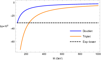
We assume that main contribution to the excited fermion masses arise at scale above EWSB and therefore we assume that they are of similar magnitude with small differences arising from SU(2) breaking contributions like couplings to exotic Higgs bosons. As already discussed, this computation is very sensitive to even small mass splittings of the SU(2) multiplets and can result in large contributions to in the form of boson self energy as shown in (15). Therefore we introduce mass splitting between the excited Fermions and study its impact on the for the doublet and triplet contributions. Here we define , , and .
Extending our analysis for the case of non degenerate masses, we show the contours of in plane in Fig. 3. We find that constrained areas by above the line (solid grey line) can be found for mass splittings larger than about 20 GeV, excluded areas with GeV (Dot-dashed green line) and GeV (Dot-dashed brown line) are shown. Area below the lower dot-dashed lines is excluded due to the lower bound on while the area above the upper dot-dashed lines is excluded by upper bound on . We have significant doublet contributions for GeV (green dot-dash line) which can result in exclusion of small area in the lower right corner of the plane due to the lower experimental bound on . Increasing the to 30 GeV not only results in the exclusion of larger part of the plane in the lower right corner of the plot but some area in the upper left corner also gets excluded, as indicated by the dot-dashed brown line, due to upper experimental limit on . We also show the experimental findings here depicting the exclusion regions in the plane with 95 C.L. Sirunyan et al. 2018; Sirunyan et al. 2019. The dashed blue line corresponds to the recent CMS search in channel with integrated luminosity of and orange line corresponds to the search for excited lepton decaying to two electrons or two muon and two jets via contact interaction with a total integrated luminosity of . The perturbative unitarity bounds for a composite fermion model were studied in Biondini et al. 2019. These bounds are depicted using purple line with decreasing thickness corresponding to 100, 95 and 50 event fractions respectively that satisfy unitarity bounds. The shaded area is excluded due to unitarity bounds (purple lines) and direct searches at the LHC (blue and orange lines).


In Fig 4, we show the in plane for the case of excited lepton triplet. In this case the space above the line (solid grey line) is constrained by for mass splittings larger than 10 GeV. Here the space above the bounds are more stringent compared to unitarity bounds even for GeV as indicated by the dot-dash black line. Increasing the mass splitting between the triplets to GeV result in the exclusion of larger area in the lower right region (area below the lower red line) as well as the upper left corner of the plot (area above the upper red line).
V Conclusions
The phenomenology of the effective interactions of a composite scenario of the standard model fermions based on extended isospin multiplets () has recently been revived with several studies of the production at LHC of the corresponding states with exotic charge such as doubly charged leptons and quarks of charge . On the other end both the ATLAS and CMS Collaborations have been testing this model at increasingly higher energies and luminosities extending the corresponding bounds in the parameter space with new analyses. Plans are laid out to further these studies at the high luminosity (HL) option of the LHC collider.
In addition to direct searches for the excited fermions at the LHC also perturbative unitarity bounds proved very effective in constraining the composite fermion models Biondini et al. 2019. In this paper, however, we have adopted yet another approach in order to constrain the excited fermion paramter space. We analyzed the effects of excited leptons to the electroweak precision observables (EWPO) in particular the parameter. As a first step, we calculated the couplings of the multiplet excited leptons to the ordinary leptons and gauge bosons and the excited lepton coupling to the excited lepton and gauge bosons. In the second step, we used these couplings to calculate the one-loop contributions to the , and self-energies for the case of the lepton triplet. These self-energy contributions were then used to estimate the value of . For the case of mass degenerate excited leptons, their contributions to turned out to be very small. However, mass splitting between the excited leptons can result in the large contributions to the coming from the boson self energy diagram. These contributions are directly proportional to the mass splitting and can results in the exclusion of significant regions in the [] plane compared to the present experimental bounds and those coming from perturbative unitarity. We believe that this study will prove helpful for the present and future experimental searches on these models.
Acknowledgements.
M. Rehman and M. E. Gomez wish to thank the Istituto Nazionale di Fisica Nucleare, INFN, Sezione di Perugia, for kind hospitality and support for collaboration visits during the early and final stages of this work. The research of M.E.G. was supported by the Spanish MINECO, under grants FPA2017-86380 and PID2019-107844GB-C22.References
- Baur et al. (1990) U. Baur, M. Spira, and P. M. Zerwas, Excited Quark and Lepton Production at Hadron Colliders, Phys. Rev. D42, 815 (1990).
- Baur et al. (1987) U. Baur, I. Hinchliffe, and D. Zeppenfeld, Excited Quark Production at Hadron Colliders, Int. J. Mod. Phys. A2, 1285 (1987).
- Aad et al. (2010) G. Aad et al. (ATLAS Collaboration), Search for new particles in two-jet final states in 7 tev proton-proton collisions with the atlas detector at the lhc, Phys. Rev. Lett. 105, 161801 (2010).
- Aad et al. (2016) G. Aad et al., Search for the production of single vector-like and excited quarks in the wt final state in pp collisions at tev with the atlas detector, Journal of High Energy Physics 2016, 110 (2016).
- Gonzalez-Garcia and Novaes (1997) M. C. Gonzalez-Garcia and S. F. Novaes, Excited fermion contribution to Z0 physics at one loop, Nucl. Phys. B486, 3 (1997), arXiv:hep-ph/9608309 [hep-ph] .
- Pancheri and Srivastava (1984) G. Pancheri and Y. N. Srivastava, Weak Isospin Spectroscopy of Excited Quarks and Leptons, Phys. Lett. 146B, 87 (1984).
- Biondini et al. (2012) S. Biondini, O. Panella, G. Pancheri, Y. N. Srivastava, and L. Fanò, Phenomenology of excited doubly charged heavy leptons at LHC, Phys. Rev. D85, 095018 (2012), arXiv:1201.3764 [hep-ph] .
- Leonardi et al. (2014) R. Leonardi, O. Panella, and L. Fanò, Doubly charged heavy leptons at LHC via contact interactions, Phys. Rev. D90, 035001 (2014), arXiv:1405.3911 [hep-ph] .
- Biondini and Panella (2015) S. Biondini and O. Panella, Exotic leptons at future linear colliders, Phys. Rev. D92, 015023 (2015), arXiv:1411.6556 [hep-ph] .
- Leonardi et al. (2016) R. Leonardi, L. Alunni, F. Romeo, L. Fanò, and O. Panella, Hunting for heavy composite Majorana neutrinos at the LHC, Eur. Phys. J. C76, 593 (2016), arXiv:1510.07988 [hep-ph] .
- Biondini et al. (2019) S. Biondini, R. Leonardi, O. Panella, and M. Presilla, Perturbative unitarity bounds for effective composite models, Phys. Lett. B 795, 644 (2019), [Erratum: Phys.Lett.B 799, 134990 (2019)], arXiv:1903.12285 [hep-ph] .
- Boudjema et al. (1993) F. Boudjema, A. Djouadi, and J. Kneur, Excited fermions at e+ e- and e P colliders, Z. Phys. C 57, 425 (1993).
- Hagiwara et al. (1985) K. Hagiwara, D. Zeppenfeld, and S. Komamiya, Excited Lepton Production at LEP and HERA, Z. Phys. C29, 115 (1985).
- Brodsky and Drell (1980) S. J. Brodsky and S. D. Drell, The Anomalous Magnetic Moment and Limits on Fermion Substructure, Phys. Rev. D22, 2236 (1980).
- Renard (1982a) F. M. Renard, Limits on Masses and Couplings of Excited Electrons and Muons, Phys. Lett. 116B, 264 (1982a).
- Renard (1982b) F. M. Renard, Tests of Composite Models With Decay Modes, Phys. Lett. 116B, 269 (1982b).
- Mertig et al. (1991) R. Mertig, M. Böhm, and A. Denner, Feyn calc - computer-algebraic calculation of feynman amplitudes, Computer Physics Communications 64, 345 (1991).
- Shtabovenko et al. (2016) V. Shtabovenko, R. Mertig, and F. Orellana, New developments in feyncalc 9.0, Computer Physics Communications 207, 432 (2016).
- Peskin and Takeuchi (1990) M. E. Peskin and T. Takeuchi, A New constraint on a strongly interacting Higgs sector, Phys. Rev. Lett. 65, 964 (1990).
- Peskin and Takeuchi (1992) M. E. Peskin and T. Takeuchi, Estimation of oblique electroweak corrections, Phys. Rev. D 46, 381 (1992).
- Tanabashi et al. (2018) M. Tanabashi et al. (Particle Data Group), Review of Particle Physics, Phys. Rev. D98, 030001 (2018).
- Sirunyan et al. (2018) A. M. Sirunyan et al. (CMS), Search for excited leptons in final states in proton-proton collisions at 13 TeV, Submitted to: JHEP (2018), arXiv:1811.03052 [hep-ex] .
- Sirunyan et al. (2019) A. M. Sirunyan et al. (CMS Collaboration), Search for excited leptons decaying via contact interaction to two leptons and two jets, (CERN, Geneva, CMS-PAS-EXO-18-013, 2019).