DCT-SNN: Using DCT to Distribute Spatial Information over Time for Learning Low-Latency Spiking Neural Networks
Abstract
Spiking Neural Networks (SNNs) offer a promising alternative to traditional deep learning frameworks, since they provide higher computational efficiency due to event-driven information processing. SNNs distribute the analog values of pixel intensities into binary spikes over time. However, the most widely used input coding schemes, such as Poisson based rate-coding, do not leverage the additional temporal learning capability of SNNs effectively. Moreover, these SNNs suffer from high inference latency which is a major bottleneck to their deployment. To overcome this, we propose a scalable time-based encoding scheme that utilizes the Discrete Cosine Transform (DCT) to reduce the number of timesteps required for inference. DCT decomposes an image into a weighted sum of sinusoidal basis images. At each time step, the Hadamard product of the DCT coefficients and a single frequency base, taken in order, is given to an accumulator that generates spikes upon crossing a threshold. We use the proposed scheme to learn DCT-SNN, a low-latency deep SNN with leaky-integrate-and-fire neurons, trained using surrogate gradient descent based backpropagation. We achieve top-1 accuracy of 89.94%, 68.3% and 52.43% on CIFAR-10, CIFAR-100 and TinyImageNet, respectively using VGG architectures. Notably, DCT-SNN performs inference with 2-14X reduced latency compared to other state-of-the-art SNNs, while achieving comparable accuracy to their standard deep learning counterparts. The dimension of the transform allows us to control the number of timesteps required for inference. Additionally, we can trade-off accuracy with latency in a principled manner by dropping the highest frequency components during inference. †† The code is available at https://github.com/SayeedChowdhury/dct-snn
1 Introduction
Deep Learning networks have tremendously improved state-of-the-art performance for many tasks such as object detection, classification and natural language processing (Krizhevsky et al. 2012; Hinton et al. 2012; Deng & Liu 2018). However, such architectures are extremely energy-intensive (Li et al. 2016) and hence, unsuitable for edge deployment. To address this, Spiking Neural Networks (SNNs) have emerged as a promising alternative to traditional deep learning architectures (Maass 1997; Roy et al. 2019). SNNs are bio-plausible networks inspired from the learning mechanisms observed in mammalian brains. They are analogous in structure to standard networks, but perform computation in the form of spikes instead of fully analog values, as done in standard networks. For the rest of this paper, we refer to standard networks as Analog Neural Networks (ANNs) to distinguish them from their spiking counterparts with digital (spiking) inputs.The input and the correspondingly generated activations in SNNs are all binary spikes and inference is performed by accumulating the spikes over time. This can be visualized as distributing the one step inference of ANNs into a multi-step, very sparse inference scheme in the SNN.
The primary source of energy efficiency of SNNs comes from the fact that very few neurons spike at any given timestep. This event driven computation and the replacement of every multiply–accumulate (MAC) operation in the ANN by an addition in SNN allows SNNs to infer with lesser energy. However, the accumulation of spikes over timesteps results in a higher inference latency in SNNs. Energy efficiency at the cost of too high a latency would still hamper real-time deployment. Consequently, reduction of timesteps required for inference in SNNs is an active field of research. One of the factors that significantly affects the number of timesteps needed is the encoding scheme that converts pixels into spikes over the timesteps. Currently, the most common encoding scheme is Poisson spike generation (Rueckauer et al. 2017), where the spikes at the input are generated as a Poisson spike train, with the mean spiking rate proportional to the pixel intensity. This scheme does not encode anything meaningful in the temporal axis and each timestep is the same as any other. Moreover, networks trained using this scheme suffer from high inference latency (Rueckauer et al. 2017). Temporal coding schemes such as phase (Kim et al. 2018) or burst (Park et al. 2019) coding have been introduced to better encode temporal information into the spike trains, but they still incur high latency and require a large number of spikes for inference. Another related temporal method is time-to-first-spike (TTFS) coding (Zhang et al. 2019; Park et al. 2020). Thy limit the number of spikes per neuron but the high latency problem still persists. Relative timing of spikes to encode information has been used in Comsa et al. 2020, but the results are only reported for simple tasks like MNIST and its scalability to deeper architectures such as VGG and more complex datasets like CIFAR remains unclear.
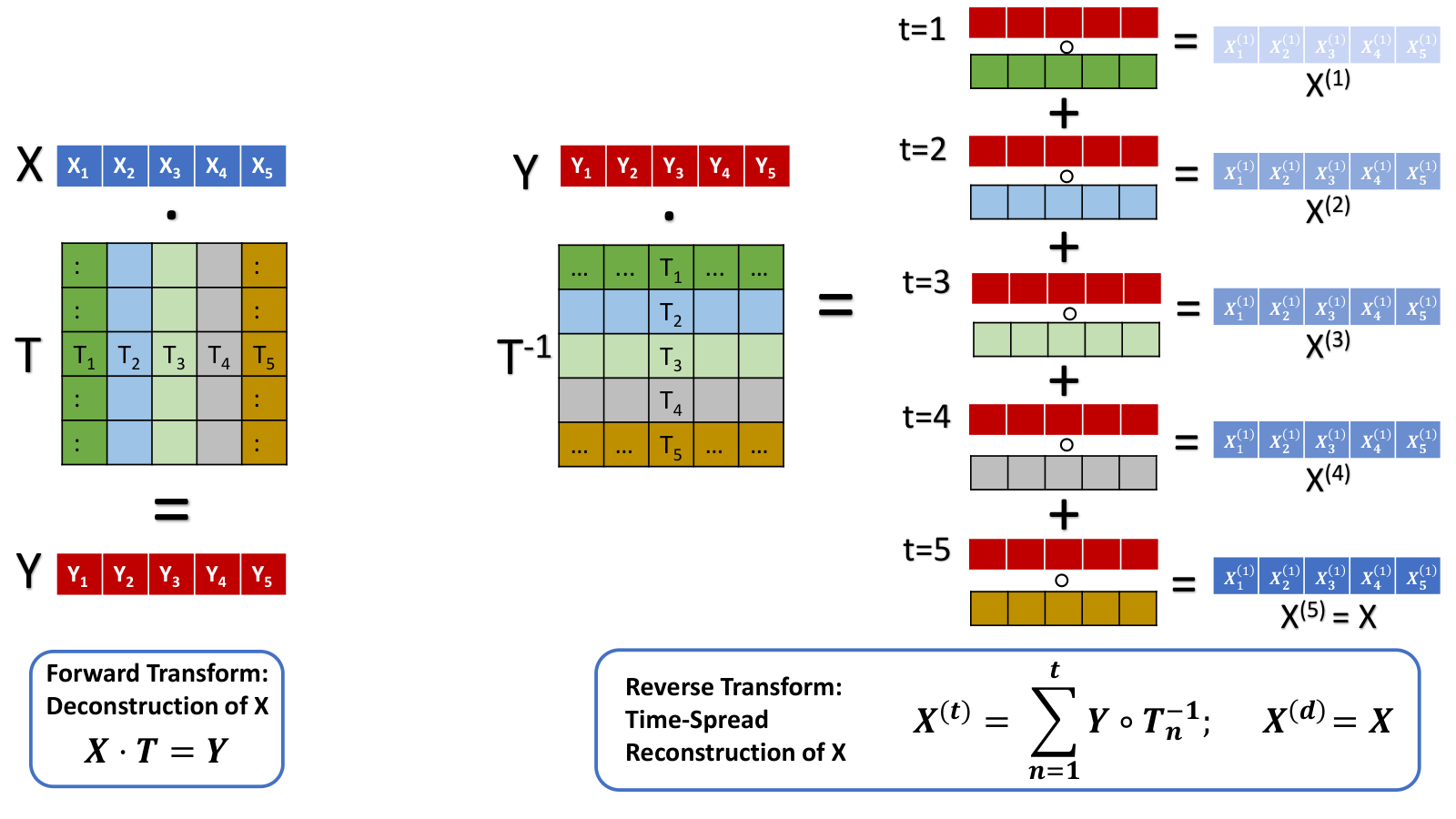
In this paper, we propose a novel encoding scheme to convert pixels into spikes over time. The proposed scheme utilizes a block-wise matrix multiplication to decompose spatial information into a weighted sum of basis, and then reverses the transform to allow reconstruction of the input over multiple timesteps. The Hadamard product of these bases, taken one per timestep, with the weights from the forward transform are then presented to the spike generating layer. The spike generator sums the contribution of all bases seen until the current timestep, as shown in Figure 1. Though any invertible matrix can be utilized as the transform, the ideal transform follows the properties of energy compaction and orthonormality of bases as outlined in Section 3.1. We motivate Discrete Cosine Transform (DCT) as the ideal choice, since it is data independent, with orthogonal bases ordered by their contribution to spectral energy. Each timestep gets the information corresponding to a single base, starting from the zero frequency component at the first timestep. Each subsequent step refines the input representation progressively. At the end of the cycle, the entire pixel value has passed through the spike generating neuron. Thus, this methodology successfully distributes the pixel value over all the timesteps in a meaningful manner. Choosing the appropriate dimensions of the transform provides a fine grained control on the number of timesteps used for inference. We use the proposed scheme to learn DCT-SNN, a spiking version of an ANN and show that it cuts down the timesteps needed to infer an image taken from CIFAR-10, CIFAR-100 and TinyImageNet datasets from 100 to 48, 125 to 48 and 250 to 48, respectively, while achieving comparable accuracy to the state-of-the-art Poisson encoded SNNs. Additionally, ordering the frequencies bases being input at each timestep provides a principled way of trading off accuracy for a reduced number of timesteps during inference, if desired, by dropping the least important (highest frequency) components.
To summarize, the main contributions of this work are as follows,
- •
A novel input encoding scheme for SNNs is introduced wherein each timestep of computation encodes distinct information, unlike other rate-encoding methods.
- •
The proposed encoding scheme is used to learn DCT-SNN, which is able to infer with 2-14X lower timesteps compared to other state-of-the-art SNNs, while achieving comparable accuracy.
- •
The proposed technique is, to the best of our knowledge, the first work that leverages frequency domain learning for SNNs on vision applications.
- •
To the best of our knowledge, this is the first work that orders timesteps by significance to reconstruction. This provides an option to trade-off accuracy for faster inference by trimming some of the later frequency components, which is non-trivial to perform in other SNNs.
2 Related Works
Learning ANNs in the frequency domain. Successful learning for vision tasks in the frequency domain has been demonstrated in ANNs in several works. These utilize the DCT coefficients directly available from JPEG compression method (Wallace 1992) without performing the decompression steps. Conventional CNNs were used with DCT coefficients as input for image classification in Ulicny & Dahyot 2017 and Rajesh et al. 2019. Ehrlich & Davis 2019 proposed a model conversion algorithm to apply pretrained spatial domain networks to JPEG images. Wavelet features are utilized in Williams & Li 2016 to train CNN-based classifiers. However, these methods suffer a small accuracy degradation compared to learning in spatial domain. DCT features were used effectively for large scale classification and instance segmentation tasks in Xu et al. 2020. Although such frequency domain approaches have proved fruitful in ANNs, it is unexplored in SNNs despite the conversion of spatial bases of the image to temporal bases in the frequency domain being intuitively related to distributing the analog pixel values in ANNs to spikes over time in SNNs.
ANN-SNN Conversion. The most common approach of training rate-coded deep SNNs is to first train an ANN and then convert it to an SNN for finetuning. (Diehl et al. 2015; Sengupta et al. 2019; Cao et al. 2015). Usually, the ANNs are trained with some limitations to facilitate this, such as not using bias, batch-norm or average pooling layers, though some works are able to bypass these constraints (Rueckauer et al. 2017). To convert ANNs to SNNs successfully, it is critical to adjust the threshold of Integrate-and-Fire (IF) / Leaky IF (LIF) neurons properly. The authors in Sengupta et al. 2019 recommend computing the layerwise thresholds as the maximum pre-activation of the neurons. This results in high accuracy but incurs high inference latency (2000-2500 timesteps). Alternatively, Rueckauer et al. 2017 choose a certain percentile of the pre-activation distribution as the threshold, reducing inference latency and improving robustness. The difference between these works and ours lie in the significance we attach to the timesteps.
Backpropagation from Scratch and Hybrid Training. Another approach to training SNNs is learning from scratch using backpropagation, which is challenging due to the non-differentiability of the spike function at the time of spike. Surrogate gradient based optimization (Neftci et al. 2019) has been utilized to circumvent this issue and implement backpropagation in SNNs effectively (Lee et al. 2020; Huh & Sejnowski 2018). Surrogate gradient based backpropagation on the membrane potential at only a single timestep was proposed in Zenke & Ganguli 2018.Shrestha & Orchard 2018 compute the gradients using the difference between the membrane potential and the threshold, but only demonstrate on MNIST using shallow architectures. (Wu et al. 2018) perform backpropagation through time (BPTT) on SNNs with a surrogate gradient defined on the membrane potential as it is continuous-valued. Overall, SNNs trained with BPTT using such surrogate-gradients have been shown to achieve high accuracy and low latency (100-125 timesteps), but the training is very compute intensive compared to conversion techniques. (Rathi et al. 2020) proposes a combination of both methods, where a pre-trained ANN serves as initialization for subsequent surrogate gradient learning in the SNN domain. This hybrid approach improves upon conversion by reducing latency and speeding up convergence. However, this is orthogonal to the encoding scheme and can be used to improve the performance of any rate-coded scheme. In this work, we adopt the hybrid training method to train the SNNs. The key distinction of our method lies in how the pixel values are encoded over time, which is described next.
3 Encoding Scheme
An ideal encoding scheme to convert pixel values into spikes over time should capture relevant information in the temporal statistics of the data. Additionally, the total spike activity over all the timesteps at the input neuron should correspond to the pixel intensity. Our encoding scheme deconstructs the image into a weighted sum of basis functions. We invert this transform to reconstruct the image over time steps. The Hadamard product of each basis function, taken one per timestep, with the weights from the deconstruction is input to an Integrate-and-Fire (IF) neuron, which accumulates the input over timesteps and fires when accumulation crosses its threshold.
3.1 A Generic 1-D Transform to Distribute Pixels over Time
1-D transformation. For simplicity, we first consider a one dimensional transform over the entire input pixel space. Let us consider a single D-dimensional image, . We transform this image using a transform matrix into a new coordinate system, where . The transformed vector, , contains the coefficients of the image in the new coordinate system. This is shown pictorially for in Figure 1. Assume that is a full rank matrix and let us consider , the inverse transformation matrix that takes us back into the original coordinate system. For reasons clarified shortly, assume that T is an orthonormal matrix with its inverse equal to its transpose, . The forward transform represents deconstruction of the input into a weighted sum of basis vectors, represented by the rows of , or columns of as shown in Figure 1. These bases are referenced by . If we input one basis function per timestep to the SNN, we get intermediate representations of the input at timestep t, by the Hadamard product of the coefficients and the -th basis, summed over all previous timesteps. Summing over all bases allows us to reconstruct X. Mathematically,
where, represents the Hadamard product, or element-wise multiplication and is the input to the spike generator at each timestep. The analog value of is converted to spikes using IF neurons as shown in Figure 3. Hence, we have successfully distributed the input X over d timesteps, with each timestep carrying information over our chosen bases. In the next section, we discuss the desirable properties of the bases for deconstructing X.
Desirable Properties of the Basis Vectors. The columns of the transform matrix contain the bases to deconstruct X. Since we use one basis per timestep, we want each base to offer non-interfering information about X. This is captured by the orthonormality constraint on T. Orthonormal columns avoid cancellation of information between timesteps, and relate the forward and reverse transforms by a transpose operation. The second constraint on T is that the bases be ranked by a measure of the information they carry. This allows each basis function to successively refine the representation per timestep. It is desirable to have the bulk of the information focused in the earlier timesteps, with fine-grained information added by the later steps. This ordering of bases allows us to drop bases in a principled manner to trade off accuracy for latency during inference.
Transforms that Satisfy Constraints. There are two widely used transforms that satisfy these properties: the DCT transform (Ahmed et al. 1974) and the Karhunen–Loève transform (Dony et al. 2001), also known as Principal Component Analysis (PCA). DCT decomposes an image into a linear combination of sinusoidal frequencies, ranked by spectral energy. PCA uses the eigenvectors of the covariance matrix of the inputs as the bases, ranked by the amount of variance they explain. DCT is commonly used in JPEG Compression and PCA in dimesionality reduction, by approximating the later components. However, PCA results in dataset dependent bases, whereas the DCT bases are pre-determined, avoiding extra computation. A comparison of the results for DCT, PCA, a random orthonormal transform without ranked bases, and a random non-orthonormal non-ranked transform is shown in Table 2. For the rest of the paper, we use the dataset agnostic DCT. Additionally, the conversion of spatial to temporal frequency in DCT lends itself intuitively to the concept of distributing spatial information in ANNs into spikes over time.


3.2 2-D Discrete Cosine Transform
We now extend the scheme to 2-D. The 2-D DCT is just the 1-D DCT applied first along the width channel and then along the length channel. Images are high dimensional, resulting in large transformation matrices . This is undesirable since the number of DCT bases (or the dimension of ) dictates the number of timesteps required to reconstruct the image. To tackle this, similar to JPEG compression scheme, we first convert the image from RGB to YCbCr domain, and then take blocks of size and perform 2-D DCT on these blocks, getting ordered frequency components. We replace the pixel block with the equivalently reshaped frequency coefficients. The DCT equations are given in appendix A.3. An block requires timesteps for perfect reconstruction of the pixel block. Small values of n allow us to reconstruct the images by summing over only a few basis images. In standard JPEG compression, blocks are used, resulting in the 64 basis images shown in Figure 3. Similarly, the bases obtained from PCA on the training dataset of CIFAR-10 are also shown. Empirically, we find that block sizes of converge to the best accuracy with the lowest number of timesteps. We usually need to run 3 full cycles to achieve convergence to best accuracy, amounting to timesteps. In each of the 3 cycles, we repeat the 16 DCT coefficients and bases, to allow time for spike propagation to the deeper layers. This is discussed in further detail in Section 4. Unlike the JPEG compression scheme, to improve accuracy we utilize an overlapped DCT scheme, where the blocks of pixels overlap. This is equivalent to performing convolution with a kernel size of 4 and a stride of 2, and increases our input dimensions by . To counter this, we add an additional average pooling layer before the linear layers.
3.3 Conversion from ANN and Threshold Selection for Spikes
In our scheme, the SNN trains on intermediate pixel representations, and hence we utilize an ANN trained with pixel intensities (rather than DCT coefficients) for initialization. The threshold of the IF neuron at the spike generator significantly affects the timesteps required for spike propagation to deeper layers. This IF neuron, as shown in Figure 3, receives the Hadamard product of the bases and DCT coefficients and accumulates them over timesteps, firing when the accumulation crosses the threshold. We allow for both positive and negative spikes to account for the positive and negative cycles of the sinusoidal bases. Similar to the hidden layer neurons, the threshold is chosen as a percentile of the accumulation at the spike generator neurons. We obtained best results by using 6.5 and 93.5 percentile of the accumulation as thresholds for negative and positive spikes, respectively.
4 Experiments and Results
We implement DCT-SNN by incorporating the proposed encoding scheme with surrogate-gradient based learning using LIF neurons. Starting with a pretrained ANN, we copy the weights to the SNN and select the 99.9 percentile of the pre-activation distribution at each layer as its threshold. The details of the learning methodology and hyperparameters of training are given in appendix section A.1 and A.2. The implementation is provided as part of the supplementary material.
Choice of Transformation. We first analyze the performance of DCT-SNN trained on different choices of transformation matrices (denoted as in section 3.1). Table 2 shows the results for a VGG5 network trained on CIFAR-10. With a random , the network does converge but with much lower accuracy than the ANN. Next, to avoid interference between different bases, we use a random orthonormal . Table 2 shows that the accuracy improves by 20% compared to non-orthonormal case. However, this choice of does not perform energy compaction. Ranking bases by their contribution to reconstruction allows us to trade off accuracy for latency during inference. To incorporate this, we experiment with the transformation matrix generated by performing PCA on blocks of the inputs from the training dataset. While this satisfies both the desired properties and gives the best performance, it is a data-dependent transform. Therefore, we utilize the fixed DCT matrix, and find that it performs at par with PCA, while additionally being data-agnostic. For all subsequent analysis, we use DCT as the choice of transformation.
|
| ||||
|---|---|---|---|---|---|
| Random | 64.7 | ||||
|
83.3 | ||||
| PCA | 83.8 | ||||
| DCT | 83.5 |
| Configuration |
|
|
| ||||||
| ANN-p | 91.3 | 69.7 | 56.9 | ||||||
| ANN-d | 90.4 | 66.4 |
| ||||||
| SNN-p |
|
67.8 (125) | 53 (250) | ||||||
| SNN-d | 88.2 (100) | 65.1 (125) | - | ||||||
| DCT-SNN |
|
|
|


Effect of Block Size and Overlap. Having chosen DCT to determine the bases of our encoding scheme, we tune the block size and stride. The results are shown in Fig. 5. ‘DCT-x’ denotes a network trained on inputs transformed with DCT of blocksize . Reducing the blocksize from 16 to 4 improves accuracy consistently. Moreover, since a blocksize of requires timesteps to pass one information of cycle, smaller blocksizes benefit from a lesser requirement of timesteps per cycle. The results on different block sizes with timesteps required in parenthesis are shown in Fig. 5. We empirically find that DCT-2 is unable to converge, and that overlapped version of DCT-4 with a stride of 2 outperforms all other cases. Hence, we utilize this scheme for all further experiments.
Number of Cycles for Information Propagation. The next design parameter is the number of timesteps per forward pass. The performance of DCT-SNN trained with different timesteps is shown in Fig. 5. In the scheme DCT-4, one full cycle amounts to 16 timesteps. The network converges to 89.94 accuracy with 48 timesteps and 88.41 accuracy with just 32 timesteps. Since performance saturates after 3 cycles (48 timesteps), we choose 48 as the number of timesteps to train DCT-SNN on CIFAR-10 and CIFAR-100. However, for deeper networks and larger datasets, larger timesteps might yield further improvements, as shown in Table 2 for TinyImagenet with VGG13. Notably, the accuracy of Poisson-encoded networks drops severely below 45 timesteps (Fig. 5), whereas DCT-SNN suffers a minimal drop even with 28 timesteps. In particular, Poisson does not converge for 32 timesteps or lesser, whereas we achieve less than 2% accuracy drop at 32 timesteps.
Results on CIFAR and TinyImageNet. The experimental results using the proposed scheme for CIFAR and TinyImageNet datasets are shown in Table 2. DCT-SNN performs comparably to SNNs trained with Poisson-encoded pixels, but requires lesser than half the timesteps. We also compare our results with SNNs trained on Poisson-encoded DCT coefficients and show that our method performs better, presumably due to the reconstruction of pixels over time. To demonstrate the scalability of the proposed algorithm, we apply it to the TinyImagenet dataset. SNNs with Poisson-encoded pixels require timesteps to converge, whereas our method can converge to comparable accuracy in 125 timesteps. Allowing for a drop in accuracy, our method converges with even 48 timesteps.
Performance Comparison with State-of-the-Art. We collect reported results for different state-of-the-art SNNs and compare our performance in Table 3. DCT-SNN performs better than or comparably to the reported accuracy of the these methods, while achieving lower latency for inference. Notably, our method also outperforms reported ANNs trained with DCT coefficients. We show two works that train ANNs on DCT coefficients. Ehrlich & Davis 2019 report ANNs with and accuracy on CIFAR-10 and CIFAR-100, respectively and Ulicny & Dahyot 2017 report accuracy on CIFAR-10. Our proposed method reaches upto , despite being an SNN. Additionally, to verify that our method is trainable via backpropagation from scratch, we trained a VGG9 SNN from scratch for CIFAR-10, which gives accuracy with 48 timesteps.
Accuracy-Latency Trade-off. The ranking of bases in our scheme allows us to drop the least significant components. In Figure 7, we show the effect the ranking of bases has on accuracy by performing inference on VGG9 DCT-SNN trained on CIFAR-10 for 48 timesteps using all 16 frequencies. A minimum of 16 timesteps (1 cycle) are required for spike propagation to the deeper layers, and hence any configuration with timesteps lesser than 16 cannot infer correctly. We provide 2 cycles of inputs on the test data. The first cycle uses all 16 components, and the next adds successively higher frequencies. Due to the fact that the bulk of the information is contained in the earlier timesteps, we are able to get good accuracy (73.9% out of 88.6% ) with just the first 4 bases. Successive components add more refined information, and therefore the accuracy saturates, as evident from Figure 7. To the best of our knowledge, this is the first work that demonstrates a principled tradeoff between inference accuracy and latency on a trained network. Results for networks trained with limited frequencies are shown in Appendix A.4.


Computational Efficiency. The floating-point (FP) MAC operations in ANN are replaced by FP additions in SNN. The cost of a MAC operation () is compared to an addition () (Horowitz 2014) in 45nm CMOS technology. The expressions representing the computational cost in the form of operations per layer in an ANN, , are given in Appendix A.5. The number of operations per layer in an equivalent DCT-SNN are related to by the layer’s spike-rate.
where spike rate is the average number of spikes per neuron per image over all timesteps in layer L. The layerwise spike rates for CIFAR-10 and CIFAR-100 using DCT-SNN are shown in Fig. 7. The overall average spike rate considering all layers for both cases is well below 5.1 (relative cost of MAC to addition), indicating the energy benefits of DCT-SNN over the corresponding ANN. For the DCT-SNN, there are additional MAC operations for 2 full precision matrix multiplications in the preprocessing step (the forward and reverse transforms). We denote these as . This computation is needed for only one cycle (16 timesteps), since the other 2 cycles just repeat the same bases and coefficients. The overhead is negligible when compared to the number of operations over all the layers across all timesteps. We compute the energy benefits of DCT-SNN over ANN, as ,
The values of are 1.52 and 1.74 for VGG9-CIFAR10 and VGG11-CIFAR100, respectively, demonstrating that DCT-SNN provides improved energy efficiency over its ANN counterpart. Similar to Park et al. 2020, the cost of memory access has not been considered in this evaluation, since it depends on the hardware architecture and system configurations.
| Reference | Dataset | Training | Architecture | Accuracy(%) | Timesteps |
|---|---|---|---|---|---|
| (Hunsberger & Eliasmith 2015) | CIFAR10 | Conversion | 2C, 2L | 82.95 | 6000 |
| (Cao et al. 2015) | CIFAR10 | Conversion | 3C, 2L | 77.43 | 400 |
| (Sengupta et al. 2019) | CIFAR10 | Conversion | VGG16 | 91.55 | 2500 |
| (Lee et al. 2020) | CIFAR10 | SGB | VGG9 | 90.45 | 100 |
| (Rueckauer et al. 2017) | CIFAR10 | Conversion | 4C, 2L | 90.85 | 400 |
| (Rathi et al. 2020) | CIFAR10 | Hybrid | VGG9 | 90.5 | 100 |
| (Park et al. 2020) | CIFAR10 | TTFS | VGG16 | 91.4 | 680 |
| (Park et al. 2019) | CIFAR10 | Burst-coding | VGG16 | 91.4 | 1125 |
| (Kim et al. 2018) | CIFAR10 | Phase-coding | VGG16 | 91.2 | 1500 |
| This work | CIFAR10 | DCT-SNN | VGG9 | 89.94 | 48 |
| (Lu & Sengupta 2020) | CIFAR100 | Conversion | VGG15 | 63.2 | 62 |
| (Rathi et al. 2020) | CIFAR100 | Hybrid | VGG11 | 67.9 | 125 |
| (Park et al. 2020) | CIFAR100 | TTFS | VGG16 | 68.8 | 680 |
| (Park et al. 2019) | CIFAR100 | Burst-coding | VGG16 | 68.77 | 3100 |
| (Kim et al. 2018) | CIFAR100 | Phase-coding | VGG16 | 68.6 | 8950 |
| This work | CIFAR100 | DCT-SNN | VGG11 | 68.3 | 48 |
| This work | TinyImagenet | DCT-SNN | VGG13 | 52.43 | 125 |
5 Conclusion
Bio-plausible SNNs offer a promising energy-efficient alternative to ANNs. The inputs to SNNs are available as spikes over time, instead of analog pixel values. The SNN derives efficiency from the sparsity of spikes per timestep, combined with their event-driven computation. However, the spike distribution over timesteps causes SNNs to have a high inference latency. The most widely used Poisson based rate encoding scheme does not encode any meaningful information into the temporal axis of SNNs, and requires a large number of timesteps for inference. To address this, we propose a new encoding scheme that can be used to distribute spatial pixel information over timesteps in an ordered fashion. The proposed scheme utilizes a linear transform in the form of an invertible matrix, with columns that serve as basis of representation distribution. The input pixels are reconstructed over time by summing the Hadamard products of these bases with the intermediate representation. At each step, we feed in the product of one of these bases, by order of their contribution, to an integrate-and-fire neuron at the input layer. As we cycle through all bases, the neuron receives the total pixel value spread over all timesteps. The ideal properties of the bases are orthonormality to avoid interference with each other, and ordering by their contribution to reconstruction of the pixel intensities. The choice of the transformation matrix are thus PCA and DCT. We chose DCT due to the frequency bases being dataset-agnostic. We get best performance with 2-D DCT on blocks of the input, resulting in 16 basis frequencies. We show that passing these 16 bases through the SNN cyclically a few times gives DCT-SNN comparable accuracy to their ANN counterparts, with less than half the number of timesteps required to learn other state-of-the-art SNNs. Additionally, ranking these bases differentiates one timestep from another. Consequently, we are able to drop the least important bases (and therefore, timesteps) and still infer, albeit with lower accuracy. This principled trade-off between inference accuracy and latency is a promising direction for deploying SNNs on edge devices.
6 Acknowledgements
This work was supported in part by the Center for Brain Inspired Computing (C-BRIC), one of the six centers in JUMP, a Semiconductor Research Corporation (SRC) program sponsored by DARPA, by the Semiconductor Research Corporation, the National Science Foundation, Intel Corporation, the DoD Vannevar Bush Fellowship, and by the U.S. Army Research Laboratory and the U.K. Ministry of Defence under Agreement Number W911NF-16-3-0001.
References
- Ahmed et al. (1974) Nasir Ahmed, T_ Natarajan, and Kamisetty R Rao. Discrete cosine transform. IEEE transactions on Computers, 100(1):90–93, 1974.
- Bellec et al. (2018) Guillaume Bellec, Darjan Salaj, Anand Subramoney, Robert Legenstein, and Wolfgang Maass. Long short-term memory and learning-to-learn in networks of spiking neurons. In Advances in Neural Information Processing Systems, pp. 787–797, 2018.
- Cao et al. (2015) Yongqiang Cao, Yang Chen, and Deepak Khosla. Spiking deep convolutional neural networks for energy-efficient object recognition. International Journal of Computer Vision, 113(1):54–66, 2015.
- Comsa et al. (2020) Iulia M Comsa, Thomas Fischbacher, Krzysztof Potempa, Andrea Gesmundo, Luca Versari, and Jyrki Alakuijala. Temporal coding in spiking neural networks with alpha synaptic function. In ICASSP 2020-2020 IEEE International Conference on Acoustics, Speech and Signal Processing (ICASSP), pp. 8529–8533. IEEE, 2020.
- Deng & Liu (2018) Li Deng and Yang Liu. Deep learning in natural language processing. Springer, 2018.
- Diehl et al. (2015) Peter U Diehl, Daniel Neil, Jonathan Binas, Matthew Cook, Shih-Chii Liu, and Michael Pfeiffer. Fast-classifying, high-accuracy spiking deep networks through weight and threshold balancing. In 2015 International Joint Conference on Neural Networks (IJCNN), pp. 1–8. ieee, 2015.
- Dony et al. (2001) R Dony et al. Karhunen-loeve transform. The transform and data compression handbook, 1:1–34, 2001.
- Ehrlich & Davis (2019) Max Ehrlich and Larry S Davis. Deep residual learning in the jpeg transform domain. In Proceedings of the IEEE International Conference on Computer Vision, pp. 3484–3493, 2019.
- Glorot & Bengio (2010) Xavier Glorot and Yoshua Bengio. Understanding the difficulty of training deep feedforward neural networks. In Proceedings of the thirteenth international conference on artificial intelligence and statistics, pp. 249–256, 2010.
- Hinton et al. (2012) Geoffrey Hinton, Li Deng, Dong Yu, George E Dahl, Abdel-rahman Mohamed, Navdeep Jaitly, Andrew Senior, Vincent Vanhoucke, Patrick Nguyen, Tara N Sainath, et al. Deep neural networks for acoustic modeling in speech recognition: The shared views of four research groups. IEEE Signal processing magazine, 29(6):82–97, 2012.
- Horowitz (2014) Mark Horowitz. 1.1 computing’s energy problem (and what we can do about it). In 2014 IEEE International Solid-State Circuits Conference Digest of Technical Papers (ISSCC), pp. 10–14. IEEE, 2014.
- Huh & Sejnowski (2018) Dongsung Huh and Terrence J Sejnowski. Gradient descent for spiking neural networks. In Advances in Neural Information Processing Systems, pp. 1433–1443, 2018.
- Hunsberger & Eliasmith (2015) Eric Hunsberger and Chris Eliasmith. Spiking deep networks with lif neurons. arXiv preprint arXiv:1510.08829, 2015.
- Kim et al. (2018) Jaehyun Kim, Heesu Kim, Subin Huh, Jinho Lee, and Kiyoung Choi. Deep neural networks with weighted spikes. Neurocomputing, 311:373–386, 2018.
- Krizhevsky et al. (2012) Alex Krizhevsky, Ilya Sutskever, and Geoffrey E Hinton. Imagenet classification with deep convolutional neural networks. In Advances in neural information processing systems, pp. 1097–1105, 2012.
- Lee et al. (2020) Chankyu Lee, Syed Shakib Sarwar, Priyadarshini Panda, Gopalakrishnan Srinivasan, and Kaushik Roy. Enabling spike-based backpropagation for training deep neural network architectures. Frontiers in Neuroscience, 14, 2020.
- Li et al. (2016) Da Li, Xinbo Chen, Michela Becchi, and Ziliang Zong. Evaluating the energy efficiency of deep convolutional neural networks on cpus and gpus. In 2016 IEEE international conferences on big data and cloud computing (BDCloud), social computing and networking (SocialCom), sustainable computing and communications (SustainCom)(BDCloud-SocialCom-SustainCom), pp. 477–484. IEEE, 2016.
- Lu & Sengupta (2020) Sen Lu and Abhronil Sengupta. Exploring the connection between binary and spiking neural networks. arXiv preprint arXiv:2002.10064, 2020.
- Maass (1997) Wolfgang Maass. Networks of spiking neurons: the third generation of neural network models. Neural networks, 10(9):1659–1671, 1997.
- Neftci et al. (2019) Emre O Neftci, Hesham Mostafa, and Friedemann Zenke. Surrogate gradient learning in spiking neural networks. IEEE Signal Processing Magazine, 36:61–63, 2019.
- Park et al. (2019) Seongsik Park, Seijoon Kim, Hyeokjun Choe, and Sungroh Yoon. Fast and efficient information transmission with burst spikes in deep spiking neural networks. In 2019 56th ACM/IEEE Design Automation Conference (DAC), pp. 1–6. IEEE, 2019.
- Park et al. (2020) Seongsik Park, Seijoon Kim, Byunggook Na, and Sungroh Yoon. T2fsnn: Deep spiking neural networks with time-to-first-spike coding. arXiv preprint arXiv:2003.11741, 2020.
- Rajesh et al. (2019) Bulla Rajesh, Mohammed Javed, Shubham Srivastava, et al. Dct-compcnn: A novel image classification network using jpeg compressed dct coefficients. In 2019 IEEE Conference on Information and Communication Technology, pp. 1–6. IEEE, 2019.
- Rathi et al. (2020) Nitin Rathi, Gopalakrishnan Srinivasan, Priyadarshini Panda, and Kaushik Roy. Enabling deep spiking neural networks with hybrid conversion and spike timing dependent backpropagation. In International Conference on Learning Representations, 2020. URL https://openreview.net/forum?id=B1xSperKvH.
- Roy et al. (2019) Kaushik Roy, Akhilesh Jaiswal, and Priyadarshini Panda. Towards spike-based machine intelligence with neuromorphic computing. Nature, 575(7784):607–617, 2019.
- Rueckauer et al. (2017) Bodo Rueckauer, Iulia-Alexandra Lungu, Yuhuang Hu, Michael Pfeiffer, and Shih-Chii Liu. Conversion of continuous-valued deep networks to efficient event-driven networks for image classification. Frontiers in neuroscience, 11:682, 2017.
- Sengupta et al. (2019) Abhronil Sengupta, Yuting Ye, Robert Wang, Chiao Liu, and Kaushik Roy. Going deeper in spiking neural networks: Vgg and residual architectures. Frontiers in neuroscience, 13:95, 2019.
- Shrestha & Orchard (2018) Sumit Bam Shrestha and Garrick Orchard. Slayer: Spike layer error reassignment in time. In Advances in Neural Information Processing Systems, pp. 1412–1421, 2018.
- Srivastava et al. (2014) Nitish Srivastava, Geoffrey Hinton, Alex Krizhevsky, Ilya Sutskever, and Ruslan Salakhutdinov. Dropout: a simple way to prevent neural networks from overfitting. The journal of machine learning research, 15(1):1929–1958, 2014.
- Ulicny & Dahyot (2017) Matej Ulicny and Rozenn Dahyot. On using cnn with dct based image data. In Proceedings of the 19th Irish Machine Vision and Image Processing conference IMVIP, 2017.
- Wallace (1992) G. K. Wallace. The jpeg still picture compression standard. IEEE Transactions on Consumer Electronics, 38(1):xviii–xxxiv, 1992.
- Werbos (1990) Paul J Werbos. Backpropagation through time: what it does and how to do it. Proceedings of the IEEE, 78(10):1550–1560, 1990.
- Williams & Li (2016) Travis Williams and Robert Li. Advanced image classification using wavelets and convolutional neural networks. In 2016 15th IEEE international conference on machine learning and applications (ICMLA), pp. 233–239. IEEE, 2016.
- Wu et al. (2018) Yujie Wu, Lei Deng, Guoqi Li, Jun Zhu, and Luping Shi. Spatio-temporal backpropagation for training high-performance spiking neural networks. Frontiers in neuroscience, 12:331, 2018.
- Xu et al. (2020) Kai Xu, Minghai Qin, Fei Sun, Yuhao Wang, Yen-Kuang Chen, and Fengbo Ren. Learning in the frequency domain. In Proceedings of the IEEE/CVF Conference on Computer Vision and Pattern Recognition, pp. 1740–1749, 2020.
- Zenke & Ganguli (2018) Friedemann Zenke and Surya Ganguli. Superspike: Supervised learning in multilayer spiking neural networks. Neural computation, 30(6):1514–1541, 2018.
- Zhang et al. (2019) Lei Zhang, Shengyuan Zhou, Tian Zhi, Zidong Du, and Yunji Chen. Tdsnn: From deep neural networks to deep spike neural networks with temporal-coding. In Proceedings of the AAAI Conference on Artificial Intelligence, volume 33, pp. 1319–1326, 2019.
Appendix A Appendix
A.1 Overall Training Methodology
A.1.1 Spiking Neuron Model
In this work, we employ the bio-plausible Leaky Integrate and Fire (LIF) model (Hunsberger & Eliasmith 2015), which is described by-
| (1) |
where denotes the membrane potential, is the input current representing the weighted summation of spike-inputs, indicates the time constant for membrane potential decay, represents membrane leakage path resistance, is the firing threshold and is resting potential. The discretized version of Eqn. 1 implemented in our work is given as-
| (2) |
| (3) |
where is the membrane potential, subscripts and represent the post and pre-neuron, respectively, t denotes timestep, is the leak constant= , represents the weight of connection between the i-th and j-th neuron, is the output spike, and is the firing threshold. As evident from Eqn. 2, whenever crosses this threshold, it is reduced by the amount , implementing a soft-reset. We implement the proposed DCT-SNN using the model described above with our encoding scheme, the code for our work is submitted as part of the supplementary material.
A.1.2 surrogate-gradient based learning
To train deep SNNs, we use surrogate-gradient based backpropagation which performs both the temporal as well as the spatial credit assignment of errors. Spatial credit assignment is achieved by spatial error distribution across all layers, while for temporal credit assignment, we unroll the network in time and employ backpropagation through time (BPTT) (Werbos 1990). The output layer neuronal dynamics is given as-
| (4) |
here the s correspond to the membrane potential of i-th neuron of final (L-th) layer. The final layer neurons do not spike, rather we just accumulate their potential over time for classification purpose. These accumulated outputs are passed through a softmax layer to obtain the class-wise probability distribution and then the cross-entropy between the true output and the network’s predicted distribution is used as loss for backpropagation. The governing equations are-
| (5) |
| (6) |
where L is the loss function, y denotes true output, z is the prediction, T is the total number of timesteps and N is the number of classes. The derivative of the loss w.r.t. to the membrane potential of the neurons in the final layer is given as-
| (7) |
and the weight updates at the output layer are done as-
| (8) |
| (9) |
where is the learning rate, and is the weight between i-th neuron at layer and j-th neuron at layer at timestep t. Since the output layer neurons are non-spiking, the non-differentiability is not an issue here. On the other hand, the hidden layer parameter update is given by-
| (10) |
where is the spike-generating function (Eqn. 3), k is layer index. We approximate the gradient of this function w.r.t. its input using the linear surrogate-gradient (Bellec et al. 2018) as-
| (11) |
where is a hyperparameter chosen as 0.3 in this work.
A.1.3 weight initialization and threshold balancing
A key component in successful implementation of SNNs is proper initialization of weights and thresholds. As mentioned in section 2 of the main manuscript, we first pre-train an analogous ANN and copy the weights to the SNN for finetuning. It is critical to balance the layerwise neuronal thresholds to achieve satisfactory performance in SNNs. One approach is to choose the maximum input to the neurons computed over all timesteps at each layer as the threshold at that corresponding layer (Sengupta et al. 2019). However, empirically, we have found this scheme to be unstable (training did not converge in some cases due to spike-vanishing in the deeper layers), hence we select the 99.9 percentile of the pre-activation distribution at each layer to be that layer’s threshold. Again, such threshold balancing has been argued to be more robust (Rueckauer et al. 2017). Notably, the threshold computation has to be performed one layer at a time and sequentially from first layer to the end. Having initialized the SNN as discussed above, we perform the surrogate-gradient based learning, the details of which is depicted in Algorithm 1. In addition, next we also provide the experimental details in appendix section A.2.
A.2 Experimental details
A.2.1 Datasets and Models
We perform our experiments on VGG9 for CIFAR10 dataset, VGG11 for CIFAR100 and VGG13 for TinyImagenet. Some comparisons with other encoding schemes are done using VGG5.
A.2.2 Training Parameters
For all datasets, we follow some standard data augmentation techniques such as padding by 4 pixels on each side, and a crop is randomly sampled from the padded image or its horizontally flipped version (with 0.5 probability of flipping). While testing, the original images are used. Both training and testing data are normalized using 0.5 as mean and standard deviation for all channels. For training the ANNs, we use cross-entropy loss with stochastic gradient descent optimization (weight decay=0.0001, mometum=0.9). In the ANN domain, VGG5, VGG9 and VGG11 are trained for a total of 300 epochs, with an initial learning rate of 0.1, which is divided by 10 at each 100-th epoch. VGG13 with TinyImagenet is trained with similar learning rate schedule, but with initial learning rate of 0.01. The ANNs are trained with some architectural constraints to avoid significant loss during subsequent ANN-SNN conversion (Diehl et al. 2015; Sengupta et al. 2019). The ANNs do not have bias terms as it increases the difficulty of threshold balancing. Again, batch-normalization is not used, rather dropout (Srivastava et al. 2014) is used as the regularizer and a constant dropout mask is used across all timesteps while training in SNN domain. Furthermore, average-pooling is used to reduce the feature map size since max-pooling causes significant information loss in SNNs (Diehl et al. 2015). During training the ANN, the weights are initialized using Xavier initialization (Glorot & Bengio 2010). After conversion, for training in the SNN domain, networks are trained for 20-30 epochs with cross-entropy loss and adam optimizer (weight decay=0.0005). Initial learning rate is kept at 0.0001, which is halved every 5 or 6 epochs. The leak constant is chosen as 0.9901 for all simulations.
A.3 Discrete Cosine Transform
A.3.1 1-D Discrete Cosine Transform
The one dimensional DCT transform uses the following equation to take the pixel values into DCT coefficients using sinusoidal bases.
| (12) |
A.3.2 2-D Discrete Cosine Transform
The equations for converting the pixels denoted by to DCT coefficients for an block are:
| (16) |
The 2 dimensional version can be thought of as a convolutional layer, whereas the 1 dimensional DCT corresponds to a fully connected layer. The sinusoidal bases can be entered as the columns of a transformation matrix the forward transform is then computed as and the reverse transform is computed as .
A.4 Training with Curtailed Frequencies
We show the effect of training with limited frequencies in Figure 8. The frequencies are repeated cyclically until the number of specified timesteps. For instance the accuracy for 8 frequencies given 3 times (24 cycles) is 69.7%. We note that during training, there is not benefit to dropping frequencies at iso-latency requirements.

A.5 Computational Cost
The equations for calculating the number of operations in a particular layer of an ANN are given by
where denote filter width (height), is number of input (output) channels, is the height (width) of the output feature map, and is the number of input (output) nodes.