Learning by Minimizing the Sum of Ranked Range
Abstract
In forming learning objectives, one oftentimes needs to aggregate a set of individual values to a single output. Such cases occur in the aggregate loss, which combines individual losses of a learning model over each training sample, and in the individual loss for multi-label learning, which combines prediction scores over all class labels. In this work, we introduce the sum of ranked range (SoRR) as a general approach to form learning objectives. A ranked range is a consecutive sequence of sorted values of a set of real numbers. The minimization of SoRR is solved with the difference of convex algorithm (DCA). We explore two applications in machine learning of the minimization of the SoRR framework, namely the AoRR aggregate loss for binary classification and the TKML individual loss for multi-label/multi-class classification. Our empirical results highlight the effectiveness of the proposed optimization framework and demonstrate the applicability of proposed losses using synthetic and real datasets.
1 Introduction
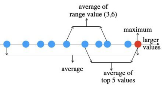
Learning objective is a fundamental component in any machine learning system. In forming learning objectives, we often need to aggregate a set of individual values to a single numerical value. Such cases occur in the aggregate loss, which combines individual losses of a learning model over each training sample, and in the individual loss for multi-label learning, which combines prediction scores over all class labels. For a set of real numbers representing individual values, the ranking order reflects the most basic relation among them. Therefore, designing learning objectives can be achieved by choosing operations defined based on the ranking order of the individual values.
Straightforward choices for such operations are the average and the maximum. Both are widely used in forming aggregate losses [35, 30] and multi-label losses [22], yet each has its own drawbacks. The average is insensitive to minority sub-groups while the maximum is sensitive to outliers, which usually appear as the top individual values. The average top- loss is introduced as a compromise between the average and the maximum for aggregate loss [11] and multi-label individual loss [12]. However, it dilutes but not exclude the influences of the outliers. The situation is graphically illustrated in Fig.1.
In this work, we introduce the sum of ranked range (SoRR) as a new form learning objectives that aggregate a set of individual values to a single value. A ranked range is a consecutive sequence of sorted values of a set of real numbers. The SoRR can be expressed as the difference between two sums of the top ranked values, which are convex functions themselves. As such, the SoRR is the difference of two convex functions and its optimization is an instance of the difference-of-convex (DC) programming problems [17]. The non-smoothness of the SoRR function and the non-convex nature of the DC programming problem can be efficiently solved with the DC algorithm (DCA).
We explore two applications in machine learning of the minimization of the SoRR framework. The first is to use the average of ranked range (AoRR) as an aggregate loss for binary classification. Unlike previous aggregate losses, the AoRR aggregate loss can completely eliminate the influence of outliers if their proportion in training data is known. Second, we use a special case of SoRR as a new type of individual loss for multi-label, the TKML loss, which explicitly encourages the true labels in the top range. The new learning objectives are tested and compared experimentally on several synthetic and real datasets11 1 Code available at https://github.com/discovershu/SoRR.. The main contributions of this work can be summarized as follows:
- •
We introduce SoRR as a general learning objective and show that it can be formulated as the difference of two convex functions, which leads to an efficient solution based on the DC algorithm.
- •
Based on SoRR, we introduce the AoRR aggregate loss for binary classification, and establish its classification calibration with regards to the optimal Bayes classifier.
- •
We also introduce the TKML individual loss for multi-label learning, which is another special case of SoRR, and show that the TKML loss is a lower bound of the conventional multi-label loss.
- •
We empirically demonstrate the robustness and effectiveness of the proposed AoRR, TKML, and their optimization framework on both synthetic and real datasets.
2 Sum of Ranked Range
For a set of real numbers , we use to denote the top- value, which is the -th largest value after sorting the elements in (ties can be broken in any consistent way). Correspondingly, we define as the sum of the top- values of . For two integers and , , the -ranked range is the set of sorted values . The sum of -ranked range (-SoRR) is defined as , and the average of -ranked range (-AoRR) is . It is easy to see that the sum of ranked range (SoRR) is the difference between two sum of top values as, . Also, the top- value corresponds to the -SoRR, as . Similarly, the median can also be obtained from AoRR, as .
In machine learning problems, we are interested in the set formed from a family of functions where each is a convex function of parameter . We can use SoRR to form learning objectives. In particular, we can eliminate the ranking operation and use the equivalent form of SoRR in the following result. Denote as the hinge function.
Theorem 1
Suppose is convex with respect to for any , then
| (1) |
Furthermore, , when the optimal solution is achieved.
The proof of Theorem 1 is in the Appendix A.1. Note that is not a convex function of . But its equivalence to the difference between and suggests that is a difference-of-convex (DC) function, because and are convex functions of in this setting. As such, a natural choice for its optimization is the DC algorithm (DCA) [27].
To be specific, for a general DC problem formed from two convex functions as , DCA iteratively search for a critical point of [33]. At each iteration of DCA, we first form an affine majorization of function using its sub-gradient at , i.e., , and then update . DCA is a descent method without line search, which means the objective function is monotonically decreased at each iteration [32]. It does not require the differentiability of and to assure its convergence. Moreover, it is known that DCA converges from an arbitrary initial point and often converges to a global solution [17]. While a DC problem can be solved based on standard (sub-)gradient descent methods, DCA seems to be more amenable to our task because of its appealing properties and the natural DC structure of our objective function. In addition, as shown in [28] with extensive experiments, DCA empirically outperforms the gradient descent method on various problems.
To use DCA to optimize SoRR, we need to solve the convex sub-optimization problem
This problem can be solved using a stochastic sub-gradient method [5, 29, 31]. We first randomly sample from the collection of and then perform the following steps:
| (2) | ||||
where is the step size. In Eq.(2), we use the fact that the sub-gradient of is computed, as
| (3) |
where is the gradient or a sub-gradient of convex function (Proof can be found in the Appendix A.2)22 2 For large datasets, we can use a stochastic version of DCA, which is more efficient with a provable convergence to a critical point [34].. The pseudo-code of minimizing SoRR is described in Algorithm 1.
3 AoRR Aggregate Loss
SoRR provides a general framework to aggregate individual values to form learning objective. Here we study in detail of its use as an aggregate loss in supervised learning problems and optimizing it with the DC algorithm. Specifically, we aim to find a parametric function with parameter that can predict a target from the input data or features using a set of labeled training samples . We assume that the individual loss for a sample as . The learning objective for supervised learning problem is constructed from the aggregate loss that accumulates all individual losses over training samples, . Specifically, we define the AoRR aggregate loss as
If we choose the individual loss or the hinge individual loss, we get the learning objectives in [25] and [14], respectively. For , we can optimize AoRR using the DCA as described in Section 2.
The AoRR aggregate loss is related with previous aggregate losses that are widely used to form learning objectives.
- •
the average loss [36]: ;
- •
the maximum loss [30]: ;
- •
the median loss [21]: ;
- •
the average top- loss (ATk) [11]: , for .
The AoRR aggregate loss generalizes the average loss ( and ), the maximum loss ( and ), the median loss (, ) , and the average top- loss (). Interestingly, the average of the bottom- loss, , which is not widely studied in the literature as a learning objective, is an instance of the AoRR aggregate loss (). In additional, the robust version of the maximum loss [30], which is a maximum loss on a subset of samples of size at least , where the number of outliers is at most , is equivalent to the top- loss, a special case of the AoRR aggregate loss ().

Using the AoRR aggregate loss can bring flexibility in designing learning objectives and alleviate drawbacks of previous aggregate losses. In particular, the average loss, the maximum loss, and the ATk loss are all influenced by outliers in training data, which correspond to extremely large individual losses. They only differ in the degree of influence, with the maximum loss being the most sensitive to outliers. In comparison, AoRR loss can completely eliminate the influence of the top individual losses by excluding the top individual losses from the learning objective.
In addition, Traditional approaches to handling outliers focus on the design of robust individual losses over training samples, notable examples include the Huber loss [13] and the capped hinge loss [23]. Changing individual losses may not be desirable, as they are usually relevant to the learning problem and application. On the other hand, the AoRR loss introduces robustness to outliers when individual losses are aggregated. The resulting learning algorithm is more flexible.
The robustness to outliers of the AoRR loss can be more clearly understood at the individual sample level, with fixed and . We use binary classification to illustrate with where is the parametric predictor and In this case, and corresponds to the correct and false predictions, respectively. Specifically, noting that , we can rearrange terms in Eq.(1) to obtain
| (4) |
We are particularly interested in the term inside the summation in Eq.(4)
According to this, at the level of individual training samples, the equivalent effect of using the AoRR loss is to uniformly reduce the individual losses by , but truncate the reduced individual loss at values below zero or above . The situation is illustrated in Fig.2 for the logistic individual loss , which is a convex and smooth surrogate to the ideal -loss. The effect of reducing and truncating from below and above has two interesting consequences. First, note that the use of convex and smooth surrogate loss inevitably introduce penalties to samples that are correctly classified but are “too close” to the boundary. The reduction of the individual loss alleviate that improper penalty. This property is also shared by the ATk loss. On the other hand, the ideal -loss exerts the same penalty to all incorrect classified samples regardless of their margin value, while the surrogate has unbounded penalties. This is the exact cause of the sensitivity to outliers of the previous aggregate losses, but the truncation of AoRR loss is similar to the -loss, and thus is more robust to the outliers. It is worth emphasizing that the above explanation of the AoRR loss has been illustrated at the individual sample level with fixed and The aggregate AoRR loss defined by (4) as a whole is not an average sample-based loss because it can not be decomposed into the summation of individual losses over samples.
3.1 Classification Calibration
A fundamental question in learning theory for classification [2, 36] is to investigate when the best possible estimator from a learning objective is consistent with the best possible, i.e., the Bayes rule. Here we investigate this statistical question for the AoRR loss by considering its infinite sample case, i.e., As mentioned above, the AoRR loss as a whole is not the average of individual losses over samples, and therefore the analysis for the standard ERM [2, 20] does not apply to our case.
We assume that the training data are i.i.d. from an unknown distribution on . The misclassification error measures the quality of a classifier is denoted by . The Bayes error leads to the least expected error, which is defined by where It is well noted that, in practice, one uses a surrogate loss which is a continuous function and upper-bounds the -loss. Its true risk is given by . Denote the optimal -risk by , the classification calibration (point-wise form of Fisher consistency) for loss [2, 20] holds true if the minimizer has the same sign as the Bayes rule , i.e., whenever .
In analogy, we can investigate the classification calibration property of the AoRR loss. Specifically, we first obtain the population form of the AoRR loss using the infinite limit of the empirical one given by Eq.(4). Indeed, we know from [4, 6] that, for any bounded and , there holds as Consequently, we have the limit case of the AoRR loss restated as follows:
| (5) | ||||
Throughout the paper, we assume that which is reasonable as In particular, we assume that since if then it will lead to and this case is reduced to the population version of average top-k case in [11]. As such, the population version of our AoRR loss (4) is given by
| (6) |
It is difficult to directly work on the optima since the problem in Eq.(6) is a non-convex min-max problem and the standard min-max theorem does not apply here. Instead, we assume the existence of and in (6) and work with the minimizer where Now we can define the classification calibration for the AoRR loss.
Definition 1
The AoRR loss is called classification calibrated if there is a minimizer such as if and if
We can then obtain the following theorem. Its proof can be found in the Appendix A.3.
Theorem 2
Suppose the individual loss is non-increasing, convex, differentiable at 0 and If , then the AoRR loss is classification calibrated.
3.2 Experiments
We empirically demonstrate the effectiveness of the AoRR aggregate loss combined with two types of individual losses for binary classification, namely, the logistic loss and the hinge loss. For simplicity, we consider a linear prediction function with parameter , and the regularizer with .


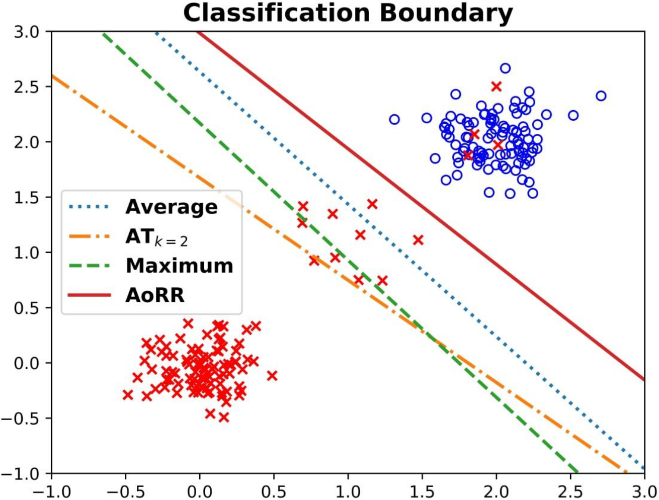
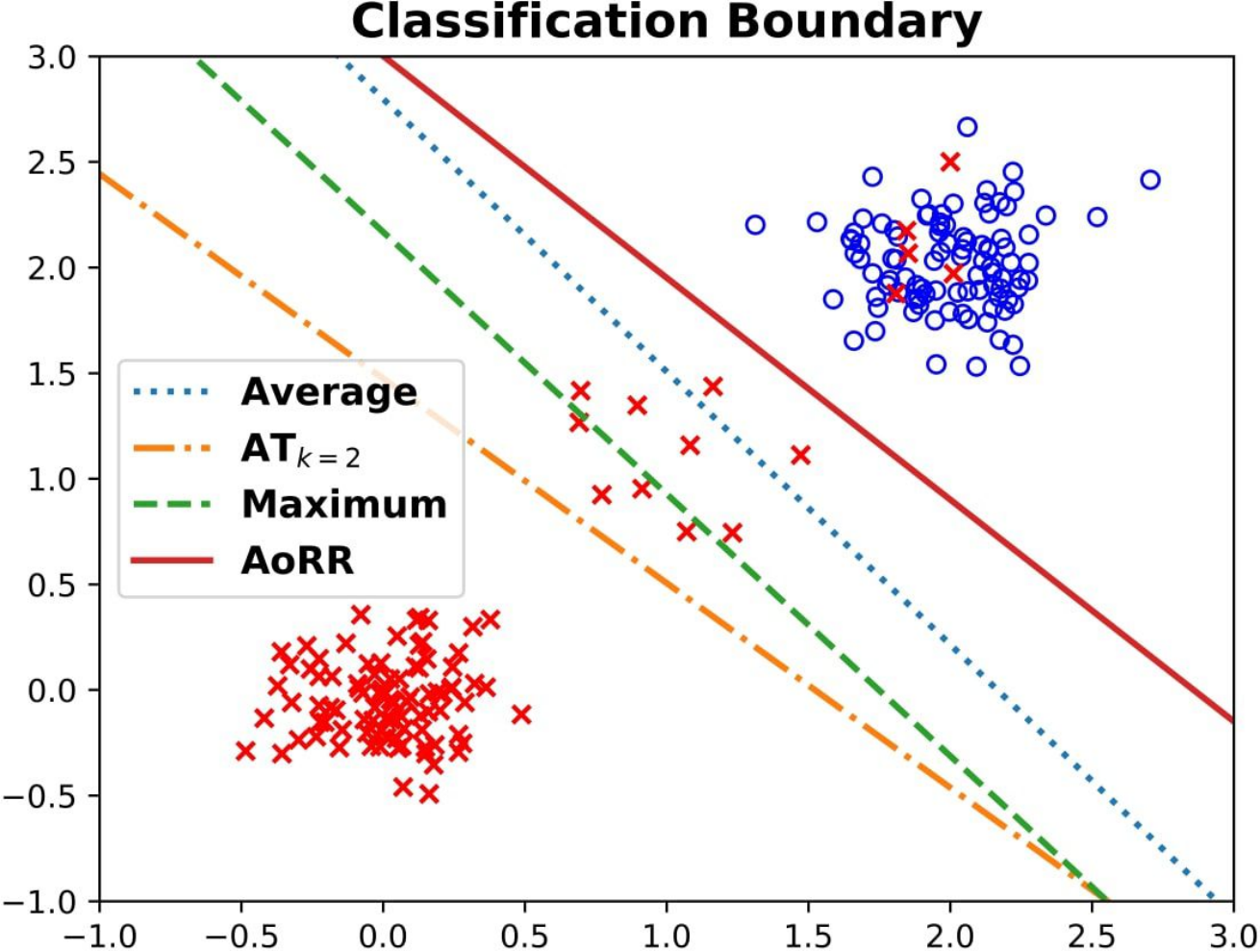
Synthetic data. We generate two sets of 2D synthetic data (Fig.3). Each dataset contains samples from Gaussian distributions with different means and variances. We consider both the case of the balanced (Fig.3 (a,b)) and the imbalanced (Fig.3 (c,d)) data distributions, in the former the training data for the two classes are approximately equal while in the latter one class has a dominating number of samples in comparison to the other. The learned linear classifiers with different aggregate losses are shown in Fig.3. Both datasets have an outlier in the blue class (shown as ). Experiments with more outliers can be found in the Appendix C.1.
To optimally remove the effect of outliers, we need to set larger than the number of outliers in the training dataset. Since there is one outlier in this synthetic dataset, we select here as an example. As shown in Fig.3, neither the maximum loss nor the average loss performs well on the synthetic dataset, due to the existence of outliers and the multi-modal nature of the data. Furthermore, Fig.3 also shows that the ATk loss does not bode well: it is still affected by outliers. The reason can be that the training process with the ATk loss with will most likely pick up one individual loss from the outlier for optimization. In contrast, the AoRR loss with =2 and =1, which is equivalent to the top- or second largest individual loss, yields better classification results. Intuitively, we avoid the direct effects of the outlier since it has the largest individual loss value. Furthermore, we perform experiments to show misclassification rates of AoRR with respect to different values of in Fig.3 (e), (f), (g), (h) for each case and compare with the ATk loss and optimal Bayes classifier. The results show that for values other than 2, the AoRR loss still exhibits an advantage over the ATk loss. Our experiments are based on a grid search for selecting the value of and because we found it is simple and often yields comparable performance. In practice for large-scale datasets, we can decide the minimal value of if we have prior knowledge about the faction of outliers in the dataset. To avoid extra freedom due to the value of , we follow a very popular adaptive setting which has been applied in previous works, (e.g., [15]). At the beginning of training, equals to the size () of training data, once training accuracy , once training accuracy , once training accuracy , once training accuracy , once training accuracy .
Real data. We use five benchmark datasets from the UCI [10] and the KEEL [1] data repositories (Statistical information of each dataset is given in the Appendix B.5). For each dataset, we first randomly select samples for training, and the remaining samples are randomly split for validation and testing (each contains 25% samples). Hyper-parameters , , and are selected based on the validation set. Specifically, parameter is chosen from , parameter , where is the number of training samples, and parameter are selected in the range of . The following results are based on the optimal values of and obtained based on the validation set. The random splitting of the training/validation/testing sets is repeated times and the average error rates, as well as the standard derivation on the testing set are reported in Table 1. In [30], the authors introduce slack variables to indicate outliers and propose a robust version of the maximum loss. We term it as Robust_Max loss and compare it to our method as one of the baselines. As these results show, comparing to the maximum, Robust_Max, average, and ATk losses, the AoRR loss achieves the best performance on all five datasets with both individual logistic loss and individual hinge loss. For individual logistic loss, the AoRR loss significantly improves the classification performance on Monk and Phoneme datasets and a slight improvement on datasets Titanic and Splice. More specifically, the performance of maximum aggregate loss is very poor on all cases due to its high sensitivity to the outliers or noisy data. The optimization of the Robust_Max loss uses convex relaxation on the domain of slack variables constraint and using norm to replace the norm in the constraint. Therefore, it can alleviate the sensitivity to outliers, but cannot exclude the influence of them. The average aggregate loss is more robust to noise and outliers than the maximum loss and the Robust_Max loss on all datasets. However, as data distributions may be very complicated, the average loss may sacrifice samples from rare distributions to pursue a lower loss on the whole training set and obtains sub-optimal solutions accordingly. The ATk loss is not completely free from the influence of outliers and noisy data either, which can be observed in particular on the Monk dataset. On the Monk dataset, in comparison to the ATk loss, the AoRR loss reduce the misclassification rates by for the individual logistic loss and for the individual hinge loss, respectively.
To further compare with the ATk loss, we investigate the influence of in the AoRR loss. Specifically, we select the best value based on the ATk results, and vary in the range of . We use the individual logistic loss and plot tendency curves of misclassification error rates w.r.t in Fig. 4, together with those from the average, maximum and Robust_Max losses. As these plots show, on all four datasets, there is a clear range of with better performance than the corresponding ATk loss. We observe a trend of decreasing error rates with increasing. This is because outliers correspond to large individual losses, and excluding them from the training loss helps improve the overall performance of the learned classifier. However, when becomes large, the classification performance is decreasing, as many samples with small losses are included in the AoRR objective and dominate the training process. The results for the individual hinge loss can be found in the Appendix C.2.
| Datasets | Logistic Loss | Hinge Loss | ||||||||
| Maximum | R_Max | Average | ATk | AoRR | Maximum | R_Max | Average | ATk | AoRR | |
| Monk | 22.41 | 21.69 | 20.46 | 16.76 | 12.69 | 22.04 | 20.61 | 18.61 | 17.04 | 13.17 |
| (2.95) | (2.62) | (2.02) | (2.29) | (2.34) | (3.08) | (3.38) | (3.16) | (2.77) | (2.13) | |
| Australian | 19.88 | 17.65 | 14.27 | 11.7 | 11.42 | 19.82 | 15.88 | 14.74 | 12.51 | 12.5 |
| (6.64) | (1.3) | (3.22) | (2.82) | (1.01) | (6.56) | (1.05) | (3.10) | (4.03) | (1.55) | |
| Phoneme | 28.67 | 26.71 | 25.50 | 24.17 | 21.95 | 28.81 | 24.21 | 22.88 | 22.88 | 21.95 |
| (0.58) | (1.4) | (0.88) | (0.89) | 5(0.71) | (0.62) | (1.7) | (1.01) | (1.01) | (0.68) | |
| Titanic | 26.50 | 24.15 | 22.77 | 22.44 | 21.69 | 25.45 | 25.08 | 22.82 | 22.02 | 21.63 |
| (3.35) | (3.12) | (0.82) | (0.84) | (0.99) | (2.52) | (1.2) | (0.74) | (0.77) | (1.05) | |
| Splice | 23.57 | 23.48 | 17.25 | 16.12 | 15.59 | 23.40 | 22.82 | 16.25 | 16.23 | 15.64 |
| (1.93) | (0.76) | (0.93) | (0.97) | (0.9) | (2.10) | (2.63) | (1.12) | (0.97) | (0.89) | |


4 Multi-label Learning
We use SoRR to construct the individual loss for multi-label/multi-class classification, where a sample can be associated with a set of labels . Our goal is to construct a linear predictor with . The final classifier outputs labels for with the top () prediction scores, i.e., . In training, the classifier is expected to include as many true labels as possible in the top outputs. This can be evaluated by the “margin”, i.e., the difference between the -th largest score of all the labels, and the lowest prediction score of all the ground-truth labels, . If we have , then all ground-truth labels have prediction scores ranked in the top positions. If this is not the case, then at least one ground-truth label has a prediction score not ranked in the top . This induces the following metric for multi-label classification as . Replacing the indicator function with the hinge function and let , where , we obtain a continuous surrogate loss, as . We term this loss as the top- multi-label (TKML) loss. When , we have the following proposition and its proof can be found in the Appendix A.4,
Proposition 1
The TKML loss is a lower-bound to the conventional multi-label loss [8], as
The TKML loss generalizes the conventional multi-class loss () and the top- consistent -guesses multi-class classification [38] (). A similar learning objective is proposed in [16] corresponds to , however, as proved in [38], it is not multi-class top- consistent. Another work in [7] proposes a robust top-k multi-class SVM based on the convex surrogate of to address the outliers by using a hyperparameter to cap the values of the individual losses. This approach is different from ours since we directly address the original top-k multi-class SVM problem using our TKML loss without introducing its convex surrogate and it is consistent. For a set of training data , if we denote , the data loss on TKML can be written as , which can be optimized using the Algorithm 1.
4.1 Experiments
We use the same regularizer, and cross-validate hyper-parameter in the range 100 to 105, extending it when the optimal value appears.
Multi-label classification. We use three benchmark datasets (Emotions, Scene, and Yeast) from the KEEL data repository to verify the effectiveness of our TKML loss. The average number of positive labels per instance in each dataset is 1.81, 1.06, and 4.22, respectively. For comparison, we compare TKML with logistic regression (LR) model (i.e. minimize a surrogate hamming loss [39]), and a ranking based method (LSEP [19]). For these two baseline methods, we use a sigmoid operator on the linear predictor as Since TKML is based on the value of , we use five different values () to evaluate the performance. For each dataset, we randomly partition it to 50%/25%/25% samples for training/validation/testing, respectively. This random partition is repeated 10 times, and the average performance on testing data is reported in Table 2. We use a metric (top multi-label accuracy) to evaluate the performance, where is the size of the sample set. For instance, with be its ground-truth set, be its predicted scores, and be a set of top predictions according to . This metric reflects the performance of a classifier can get as many true labels as possible in the top range. More details about these three datasets and settings can be found in the Appendix B.7 and B.8.
From Table 2, we note that the TKML loss in general improves the performance on the Emotions dataset for all different values. These results illustrate the effectiveness of the TKML loss. More specifically, our TKML method obtains 4.63% improvement on and 4.42% improvement on when comparing to LR. This rate of improvement becomes higher (6.26% improvement on ) when compare to LSEP. We also compare the performance of the method based on the TKML loss on different values. If we choose the value of close to the number of the ground-truth labels, the corresponding classification method outperforms the two baseline methods. For example, in the case of the Emotions dataset, the average number of positive labels per instance is , and our method based on the TKML loss achieves the best performance for . As another example, the average number of true labels for the Yeast dataset is 4.22, so the method based on the TKML loss achieves the best performance for . We provide more experiments in Appendix C.3.
Robustness analysis. As a special case of AoRR, the TKML loss exhibit similar robustness with regards to outliers, which can be elucidated with experiments in the multi-class setting (i.e., =1 and =1). We use the MNIST dataset[18], which contains training samples and testing samples that are images of handwritten digits. To simulate outliers caused by errors occurred when labeling the data, as in the work of [37], we use the asymmetric (class-dependent) noise creation method [26, 40] to randomly change labels of the training data (27, 38, 56, and 71) with a given proportion. The flipping label is chosen at random with probability . As a baseline, we use the top- multi-class SVM (SVMα) [16]. The performance is evaluated with the top 1, top 2, , top 5 accuracy on the testing samples.
| Datasets | Methods | =1 | =2 | =3 | =4 | =5 |
| Emotions | LR | 73.54(3.98) | 57.48(3.35) | 73.20(4.69) | 86.60(3.02) | 96.46(1.71) |
| LSEP | 72.18(4.56) | 55.85(3.37) | 72.18(3.74) | 85.58(2.92) | 95.85(1.07) | |
| TKML | 76.80(2.66) | 62.11(2.85) | 77.62(2.81) | 90.14(2.22) | 96.94(0.63) | |
| Scene | LR | 73.2(0.57) | 85.31(0.47) | 94.79(0.79) | 97.88(0.63) | 99.7(0.30) |
| LSEP | 69.22(3.43) | 83.83(4.83) | 92.46(4.78) | 96.35(3.5) | 98.56(1.94) | |
| TKML | 74.06(0.45) | 85.36(0.79) | 88.92(1.47) | 91.94(0.87) | 95.01(0.61) | |
| Yeast | LR | 77.57(0.91) | 70.59(1.16) | 52.65(1.23) | 43.26(1.16) | 43.49(1.33) |
| LSEP | 75.5(1.03) | 66.84(2.9) | 49.72(1.26) | 41.90(1.91) | 43.01(1.02) | |
| TKML | 76.94(0.49) | 67.19(2.79) | 45.41(0.71) | 43.47(1.06) | 44.69(1.14) |
From Table 3, it is clear that our method TKML consistently outperforms the baseline SVMα among all top 1-5 accuracies. The gained improvement in performance is getting more significant as the level of noise increases. Since our flipping method only works between two different labels, we expected the performance of TKML has some significant improvements on top 1 and 2 accuracies. Indeed, this expectation is correctly verified as Table 3 clearly indicates that the performance of our method is better than SVMα by nearly 7% accuracy (see Top-1 accuracy in the noise level 0.4). These results also demonstrate our optimization framework works well. More experiments can be found in the Appendix C.4.
| Noise Level | Methods | Top-1 Accuracy | Top-2 Accuracy | Top-3 Accuracy | Top-4 Accuracy | Top-5 Accuracy |
| 0.2 | SVMα | 78.33(0.18) | 90.66(0.29) | 95.12(0.2) | 97.28(0.09) | 98.49(0.1) |
| TKML | 83.06(0.94) | 94.17(0.19) | 97.24(0.13) | 98.47(0.05) | 99.22(0.01) | |
| 0.3 | SVMα | 74.65(0.17) | 89.31(0.24) | 94.14(0.2) | 96.73(0.23) | 98.19(0.07) |
| TKML | 80.13(1.24) | 93.37(0.1) | 96.81(0.22) | 98.21(0.05) | 99.08(0.05) | |
| 0.4 | SVMα | 68.32(0.32) | 86.71(0.42) | 93.14(0.49) | 96.16(0.32) | 97.84(0.18) |
| TKML | 75(1.15) | 92.41(0.14) | 96.2(0.13) | 97.95(0.1) | 98.89(0.04) |
5 Conclusion
In this work, we introduce a general approach to form learning objectives, i.e., sum of ranked range, which corresponds to the sum of a consecutive sequence of sorted values of a set of real numbers. We show that SoRR can be expressed as the difference between two convex problems and optimized with the difference-of-convex algorithm (DCA).
We explore two applications in machine learning of the minimization of the SoRR framework, namely the AoRR aggregate loss for binary classification and the TKML individual loss for multi-label/multi-class classification. Our empirical results showed the effectiveness of the proposed framework on achieving superior generalization and robust performance on synthetic and real datasets. For future works, we plan to further study the consistency of TKML loss for multi-label learning and incorporate SoRR into the learning of deep neural networks.
6 Broader Impact
Loss functions are fundamental components in any machine learning system. Our work, by designing new types of loss functions based on the use of SoRR , is expected to be applicable to a wide range of ML problems. The benefit of using our method is the better handling of potential outliers in the training dataset, which could be the result of gross error or intentional “poisoning” of the dataset. However, there is also a risk of resulting a biased learning model when certain training samples are excluded. To mitigate such risks, we encourage further study to understand the impacts of using SoRR based losses in particular real-world scenarios, focusing on the more contextually meaning choice of the values and for better tradeoff of robustness and bias.
Acknowledgments. We are grateful to all anonymous reviewers for their constructive comments. This work is supported by NSF research grants (IIS-1816227 and IIS-2008532) as well as an Army Research Office grant (agreement number: W911 NF-18-1-0297).
References
- [1] J. Alcalá-Fdez, A. Fernández, J. Luengo, J. Derrac, S. García, L. Sánchez, and F. Herrera. Keel data-mining software tool: data set repository, integration of algorithms and experimental analysis framework. Journal of Multiple-Valued Logic & Soft Computing, 17, 2011.
- [2] P. L. Bartlett, M. I. Jordan, and J. D. McAuliffe. Convexity, classification, and risk bounds. Journal of the American Statistical Association, 101(473):138–156, 2006.
- [3] D. P. Bertsekas. Control of uncertain systems with a set-membership description of the uncertainty. PhD thesis, Massachusetts Institute of Technology, 1971.
- [4] S. P. Bhat and L. Prashanth. Concentration of risk measures: A wasserstein distance approach. In Advances in Neural Information Processing Systems, pages 11739–11748, 2019.
- [5] L. Bottou and O. Bousquet. The tradeoffs of large scale learning. In Advances in neural information processing systems, pages 161–168, 2008.
- [6] D. B. Brown. Large deviations bounds for estimating conditional value-at-risk. Operations Research Letters, 35(6):722–730, 2007.
- [7] X. Chang, Y.-L. Yu, and Y. Yang. Robust top-k multiclass svm for visual category recognition. In Proceedings of the 23rd ACM SIGKDD International Conference on Knowledge Discovery and Data Mining, pages 75–83, 2017.
- [8] K. Crammer and Y. Singer. A family of additive online algorithms for category ranking. Journal of Machine Learning Research, 3(Feb):1025–1058, 2003.
- [9] J. M. Danskin. The theory of max-min and its application to weapons allocation problems, volume 5. Springer Science & Business Media, 2012.
- [10] D. Dua and C. Graff. UCI machine learning repository, 2017.
- [11] Y. Fan, S. Lyu, Y. Ying, and B. Hu. Learning with average top-k loss. In Advances in neural information processing systems, pages 497–505, 2017.
- [12] Y. Fan, B. Wu, R. He, B.-G. Hu, Y. Zhang, and S. Lyu. Groupwise ranking loss for multi-label learning. IEEE Access, 8:21717–21727, 2020.
- [13] J. Friedman, T. Hastie, and R. Tibshirani. The elements of statistical learning, volume 1. Springer series in statistics New York, 2001.
- [14] T. Kanamori, S. Fujiwara, and A. Takeda. Robustness of learning algorithms using hinge loss with outlier indicators. Neural Networks, 94:173–191, 2017.
- [15] K. Kawaguchi and H. Lu. Ordered sgd: A new stochastic optimization framework for empirical risk minimization.
- [16] M. Lapin, M. Hein, and B. Schiele. Top-k multiclass svm. In Advances in Neural Information Processing Systems, pages 325–333, 2015.
- [17] H. A. Le Thi and T. P. Dinh. Dc programming and dca: thirty years of developments. Mathematical Programming, 169(1):5–68, 2018.
- [18] Y. LeCun, L. Bottou, Y. Bengio, and P. Haffner. Gradient-based learning applied to document recognition. Proceedings of the IEEE, 86(11):2278–2324, 1998.
- [19] Y. Li, Y. Song, and J. Luo. Improving pairwise ranking for multi-label image classification. In Proceedings of the IEEE conference on computer vision and pattern recognition, pages 3617–3625, 2017.
- [20] Y. Lin. A note on margin-based loss functions in classification. Statistics & probability letters, 68(1):73–82, 2004.
- [21] Y. Ma, L. Li, X. Huang, and S. Wang. Robust support vector machine using least median loss penalty. IFAC Proceedings Volumes, 44(1):11208–11213, 2011.
- [22] G. Madjarov, D. Kocev, D. Gjorgjevikj, and S. Džeroski. An extensive experimental comparison of methods for multi-label learning. Pattern recognition, 45(9):3084–3104, 2012.
- [23] F. Nie, X. Wang, and H. Huang. Multiclass capped lp-norm svm for robust classifications. In Thirty-First AAAI Conference on Artificial Intelligence (AAAI 2017), 2017.
- [24] W. Ogryczak and A. Tamir. Minimizing the sum of the k largest functions in linear time. Information Processing Letters, 85(3):117–122, 2003.
- [25] A. Ortis, G. M. Farinella, and S. Battiato. Predicting social image popularity dynamics at time zero. IEEE Access, 7:171691–171706, 2019.
- [26] G. Patrini, A. Rozza, A. Krishna Menon, R. Nock, and L. Qu. Making deep neural networks robust to label noise: A loss correction approach. In Proceedings of the IEEE Conference on Computer Vision and Pattern Recognition, pages 1944–1952, 2017.
- [27] D. N. Phan. DCA based algorithms for learning with sparsity in high dimensional setting and stochastical learning. PhD thesis, 2016.
- [28] B. Piot, M. Geist, and O. Pietquin. Difference of convex functions programming applied to control with expert data. arXiv preprint arXiv:1606.01128, 2016.
- [29] A. Rakhlin, O. Shamir, and K. Sridharan. Making gradient descent optimal for strongly convex stochastic optimization. arXiv preprint arXiv:1109.5647, 2011.
- [30] S. Shalev-Shwartz and Y. Wexler. Minimizing the maximal loss: How and why. In ICML, pages 793–801, 2016.
- [31] N. Srebro and A. Tewari. Stochastic optimization for machine learning. ICML Tutorial, 2010.
- [32] P. D. Tao and L. T. H. An. Convex analysis approach to dc programming: theory, algorithms and applications. Acta mathematica vietnamica, 22(1):289–355, 1997.
- [33] H. A. L. Thi, H. M. Le, D. N. Phan, and B. Tran. Stochastic dca for the large-sum of non-convex functions problem and its application to group variable selection in classification. In Proceedings of the 34th International Conference on Machine Learning-Volume 70, pages 3394–3403. JMLR. org, 2017.
- [34] H. A. L. Thi, H. M. Le, D. N. Phan, and B. Tran. Stochastic dca for minimizing a large sum of dc functions with application to multi-class logistic regression. arXiv preprint arXiv:1911.03992, 2019.
- [35] V. Vapnik. Principles of risk minimization for learning theory. In Advances in neural information processing systems, pages 831–838, 1992.
- [36] V. Vapnik. The nature of statistical learning theory. Springer science & business media, 2013.
- [37] Y. Wang, X. Ma, Z. Chen, Y. Luo, J. Yi, and J. Bailey. Symmetric cross entropy for robust learning with noisy labels. In Proceedings of the IEEE International Conference on Computer Vision, pages 322–330, 2019.
- [38] F. Yang and S. Koyejo. On the consistency of top-k surrogate losses. arXiv preprint arXiv:1901.11141, 2019.
- [39] M.-L. Zhang and Z.-H. Zhou. A review on multi-label learning algorithms. IEEE transactions on knowledge and data engineering, 26(8):1819–1837, 2013.
- [40] Z. Zhang and M. Sabuncu. Generalized cross entropy loss for training deep neural networks with noisy labels. In Advances in neural information processing systems, pages 8778–8788, 2018.
Appendix
Appendix A Proofs
A.1 Proof of Theorem 1
To prove Theorem 1, we need the following lemma.
Lemma 1 ([24])
. is a convex function of the elements of . Furthermore, for any , we have , of which is an optimum solution.
Proof of Theorem 1
Proof: From Lemma 1, we have
If the optimal solution is achieved, from Lemma 1, we get and . Therefore, because .
A.2 Proof of Equation (3)
Before introducing the sub-gradient of , we provide a very useful characterization of differentiable properties of the optimal value function [3, Proposition A.22], which is also an extension of Danskin’s theorem [9].
Lemma 2
Let be a function and let be a compact subset of . Assume further that for every vector the function is a closed proper convex function. Consider the function defined as , then if is finite somewhere, it is a closed proper convex function. Furthermore, if int and is continuous on the set int, then for every we have , where is the set
Proof of Equation (3)
Proof: We apply Lemma 2 with a new notation . Suppose and , the function . Let Y be a compact subset of and for every , it is obviously that the function is a closed proper convex function w.r.t from the second term of Eq.(1).
Consider a function defined as , since is finite somewhere, it is a closed proper convex function. The interior of the effective domain of is nonempty, and that is continuous on the set . The condition of lemma 2 is satisfied.
, we have
where
As we know . This means the subdifferential of w.r.t exists when we set the optimal value of .
From the above and the lemma 1, we can get the sub-gradient , where equals to .
A.3 Proof of Theorem 2
Proof: Without loss of generality, by normalization we can assume which can be satisfied by scaling. For any fixed , by the definition of , we know that
Notice the assumption and recall We need to show that for and if Indeed, if , then, by the definition of , we have that
The above inequality is identical to
Since , we have that that is a non-decreasing function of variable . Then, if we must have which indicates From the non-increasing property of on , is also a convex function and immediately indicates . Likewise, we can show that for
To prove is not a minimizer, without loss of generality, assume . We need to consider two conditions as follows,
1. If and , then
Since and is non-increasing, there exists , and . Let
Then
Therefore, is not a minimizer.
2. If and , then
Thus is not a minimizer.
A.4 Proof of Proposition 1
Proof: We just need to prove that . If this is not the case, then for any label , then its rank in the ranked list is no more than , then the sum of total number of such labels is not larger than . And the total number of labels will be , which is a contradiction.
Appendix B Additional Experimental Details
B.1 Source Code
For the purpose of review, the source code and datasets are accessible at supplementary file.
B.2 Computing Infrastructure Description
All algorithms are implemented in Python 3.6 and trained and tested on an Intel(R) Xeon(R) CPU W5590 @3.33GHz with 48GB of RAM.
B.3 Time Complexity Analyze
We consider the average case in the time complexity analyze. For a given outer loop size , a inner loop size , and training sample size , the complexity of our MSoRR Algorithm 1 is .
B.4 Training Settings on Toy Examples for Aggregate Loss
To reproduce the experimental results of AoRR on synthetic data, we provide the details about the settings when we are training the model in Table 4. For example, the learning rate, the number of epochs for the outer loop, and the number of epochs for the inner loop.
| Datasets | Outliers | Logistic loss | Hinge loss | ||||
| LR | # OE | # IE | LR | # OE | # IE | ||
| Multi-modal data | 1 | 0.01 | 100 | 1000 | 0.01 | 5 | 1000 |
| 2 | 0.01 | 100 | 1000 | 0.01 | 5 | 1000 | |
| 3 | 0.01 | 100 | 1000 | 0.01 | 5 | 1000 | |
| 4 | 0.01 | 100 | 1000 | 0.01 | 5 | 1000 | |
| 5 | 0.01 | 100 | 1000 | 0.01 | 5 | 1000 | |
| 10 | 0.01 | 100 | 1000 | 0.01 | 5 | 1000 | |
| 20 | 0.01 | 100 | 1000 | 0.01 | 5 | 1000 | |
| Imbalanced data | 1 | 0.01 | 100 | 1000 | 0.01 | 5 | 1000 |
- *
LR: Learning Rate, OE: Outer Epochs, IE: Inner epochs
B.5 Description of Datasets for Aggregate Loss
In aggregate loss experiments, for real-world datasets, we use five benchmark datasets from the UCI and the KEEL data repositories. The details of these datasets are shown in Table 5.
| Datasets | #Classes | #Samples | #Features | Class Ratio |
| Monk | 2 | 432 | 6 | 1.12 |
| Australian | 2 | 690 | 14 | 1.25 |
| Phoneme | 2 | 5,404 | 5 | 2.41 |
| Titanic | 2 | 2,201 | 3 | 2.10 |
| Splice | 2 | 3,175 | 60 | 1.08 |
B.6 Training Settings on Real Datasets for Aggregate Loss
We provide a reference for setting parameters to reproduce our AoRR experiments on real datasets. Table 6 contains the settings for individual logistic loss. Table 7 is for individual hinge loss.
| Datasets | # Outer epochs | # Inner epochs | Learning rate | |||
| Monk | 70 | 20 | 5 | 2000 | 0.01 | |
| Australian | 80 | 3 | 10 | 1000 | 0.01 | |
| Phoneme | 1400 | 100 | 10 | 1000 | 0.01 | |
| Titanic | 500 | 10 | 10 | 1000 | 0.01 | |
| Splice | 450 | 50 | 10 | 1000 | 0.01 |
| Datasets | # Outer epochs | # Inner epochs | Learning rate | |||
| Monk | 70 | 45 | 5 | 1000 | 0.01 | |
| Australian | 80 | 3 | 5 | 1000 | 0.01 | |
| Phoneme | 1400 | 410 | 10 | 500 | 0.01 | |
| Titanic | 500 | 10 | 5 | 500 | 0.01 | |
| Splice | 450 | 50 | 10 | 1000 | 0.01 |
B.7 Description of Datasets for Multi-label Learning
In multi-label learning experiments, we conduct experiments on three benchmark datasets (Emotions, Scene and Yeast) from the KEEL data repository. The details of them as described in Table 8.
| Datasets | #Samples | #Features | #Labels | |
| Emotions | 593 | 72 | 6 | 1.81 |
| Scene | 2,407 | 294 | 6 | 1.06 |
| Yeast | 2,417 | 103 | 14 | 4.22 |
B.8 Training Settings for Multi-label Learning
The settings for TKML on three real datasets are shown in Table 9.
| Datasets | #Outer epochs | #Inner epochs | Learning rate | |
| Emotions | 20 | 1000 | 0.1 | |
| Scene | 20 | 1000 | 0.1 | |
| Yeast | 20 | 1000 | 0.1 |
B.9 Training Settings for Multi-class Learning
Training settings for the MNIST dataset in different noise level can be found in Table 10.
| Noise level | #Outer epochs | #Inner epochs | Learning rate |
| 0.2 | 27 | 2000 | 0.1 |
| 0.3 | 25 | 2000 | 0.1 |
| 0.4 | 21 | 2000 | 0.1 |
Appendix C Additional Experimental Results
C.1 Toy Examples with More Outliers for Effects of Aggregate Losses
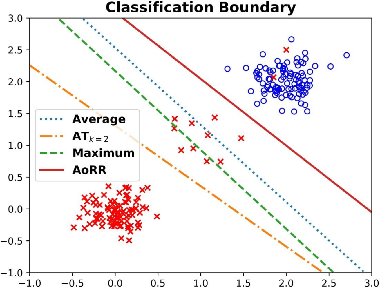
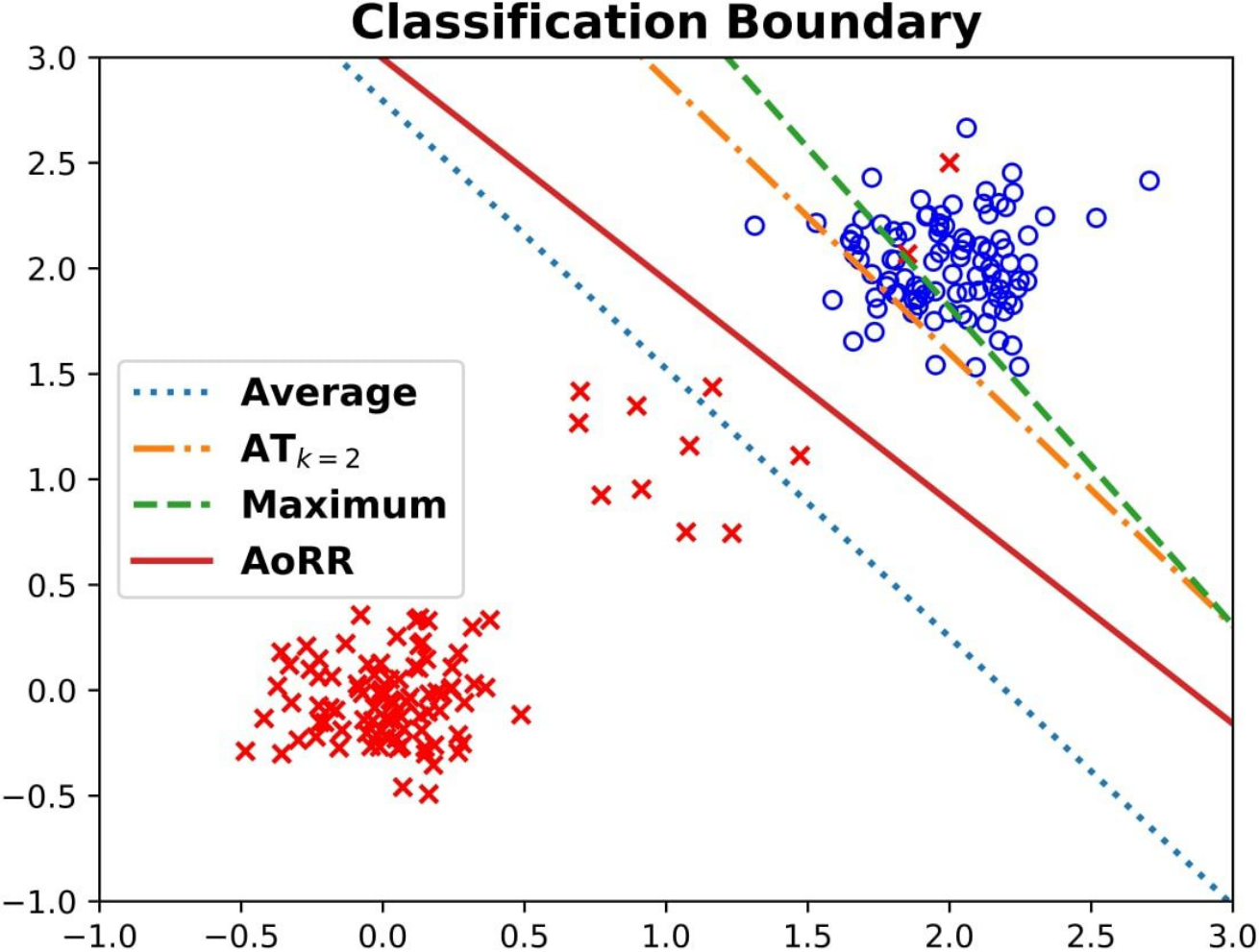
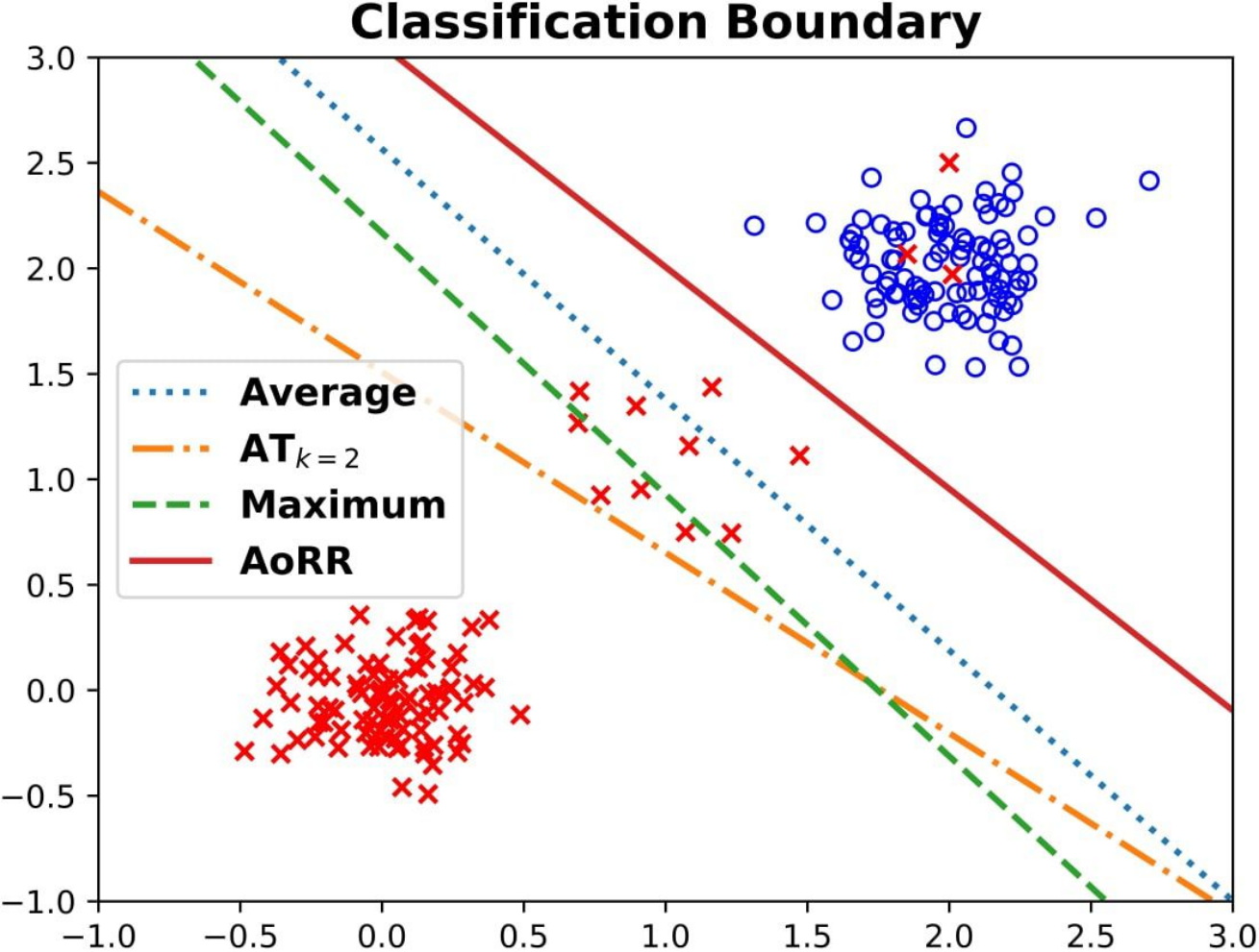
In order to evaluate the effects of different aggregate losses on more than one outlier, we also conducted additional experiments on a multi-modal toy example with outliers. We use Gaussian distributions with the different mean and standard deviations to generate this dataset (Fig.5). It contains 200 samples and is distributed in 2 classes (100 samples in red class and 100 samples in blue class). The red samples are sampled from two distributions (primary distribution and minor distribution). The blue samples are sampled from only one distribution. However, they can still be separated. A linear classifier is considered and different aggregate losses are evaluated in individual logistic loss (i.e., Fig.5 (a), (c), (e), (g), (i), (k)) and individual hinge loss (i.e., Fig.5 (b), (d), (f), (h), (j), (l)). Given a number , we set outliers as replacing blue samples class with the opposite class. The outliers have been shown as in blue class. For ATk and AoRR losses, we let the value of be the same and equals to . Let the value of equals to in AoRR loss. We consider six cases as follows,
Case 1 (2 outliers). In Fig.5 (a) and (b), there exist two outliers. Let hyper-parameters and .
Case 2 (3 outliers). Fig.5 (c) and (d) contain three outliers. In this scenario, and .
Case 3 (4 outliers). Fig.5 (e) and (f) include four outliers and we set and .
Case 4 (5 outliers). There are five outliers in Fig.5 (g) and (h). We set and .
Case 5 (10 outliers). Ten outliers have been included in Fig.5 (i) and (j). Let and in this case.
Case 6 (20 outliers). We create twenty outliers in Fig.5 (k) and (l) and make and .
See from case 1, 2, 3, 4, the linear classifier learned from average aggregate loss cross some red samples from minor distribution even though the data is separable. The reason is that the samples close to the decision boundary are sacrificed to reduce the total loss over the whole dataset.
Since the value is set to be , the ATk loss select largest individual losses which contain many outliers to train the classifier. It leads to the instability of the learned classifier. This phenomenon can be found when we compare all cases. Similarly, the maximum aggregate loss cannot fit this data very well in all cases. This loss is very sensitive to outliers.
From cases 5 and 6, the average aggregate loss with individual logistic loss achieves better results than with individual hinge loss. A possible reason is that for correctly classified samples with a margin greater than 1, the penalty caused by hinge loss is 0. However, it is non-zero when using logistic loss. Since many outliers in blue class, to reduce the average loss, the decision boundary will close to blue class. Especially, when we compare (i) and (k), it is obvious that average loss can achieve a better result while the number of outliers is increasing.
As we discussed, hinge loss has less penalty for correctly classified samples than logistic loss. This causes outliers to be more prominent than normal samples while using the individual hinge loss. This analysis can be verified in the experiment when we compare the individual logistic loss and the individual hinge loss. For example, (i) and (j), (k) and (l), etc.. We find the decision boundaries of maximum loss and ATk loss are close to outliers in the individual hinge loss scenario because both of them are sensitive to outliers in our cases.




C.2 Additional Tendency Curves for Effects of Aggregate Losses


In this section, we use individual hinge loss as an example and plot tendency curves of the error rate w.r.t in Fig.6 on 4 real-world datasets. From this figure, we get similar results as we discussed before.
C.3 Performance of Additional Evaluation Metric on TKML
We also adopt a widely used multi-label learning metric named average precision (AP) for performance evaluation. It is calculated as [39]
where returns the rank of in descending according to .
From Table 11, we can find our TKML method outperforms the other two baseline approaches on all datasets. For the Emotions dataset, the AP score of TKML is 2.16% higher than the LSEP method and near 10% higher than the LR. The performance is also slightly improved on Scene and Yeast datasets. These results demonstrate the effectiveness of our TKML method.
| Emotions | Scene | Yeast | |
| LR | 74.85 | 71.6 | 73.56 |
| LSEP | 82.66 | 85.43 | 74.26 |
| TKML | 84.82 | 86.38 | 74.32 |
C.4 Performance on Each Class of the MNIST for Effects of TKML


Performance on each class. To evaluate our method is better than SVMα on the noisy data, we plot the class-wise error rate w.r.t different noise level data. As seen in Figure 7, our method TKML outperforms SVMα on the flipping classes such as 2 and 3, especially in class 5. As the noise level increases, the performance gap becomes more pronounced. For flipping class 7, the performance in this class is increased when the noise level increases from 0.3 to 0.4. The flipping class 6 also get good performance on the noise level 0.2 and 0.3.