Learning Risk Preferences from Investment Portfolios Using Inverse Optimization

Shi Yu Affiliation: The Vanguard Group , Malvern , USA , Haoran Wang Affiliation: The Vanguard Group , Malvern , USA email: shi_yu,haoran_wang@vanguard.com and Chaosheng Dong Affiliation: Amazon , Seattle , USA email: chaosd@amazon.com

Abstract.

The fundamental principle in Modern Portfolio Theory (MPT) is based on the quantification of the portfolio’s risk related to performance. Although MPT has made huge impacts to the investment world and prompted the success and prevalence of passive investing, it still has shortcomings in real-world applications. One of the main challenges is that the level of risk an investor can endure, known as risk-preference, is a subjective choice that is tightly related to psychology and behavioral science in decision making. This paper presents a novel approach of measuring risk preference from existing portfolios using inverse optimization on mean-variance portfolio allocation framework. Our approach allows the learner to continuously estimate real-time risk preferences using concurrent observed portfolios and market price data. We demonstrate our methods on robotic investment portfolios and real market data that consists of 20 years of asset pricing and 10 years of mutual fund portfolio holdings. Moreover, the quantified risk preference parameters are validated with two well-known risk measurements currently applied in the field. The proposed methods could lead to practical and fruitful innovations in automated/personalized portfolio management, such as Robo-advising, to augment financial advisors’ decision intelligence in a long-term investment horizon.

Keywords:

Inverse Optimization, Risk Preference, Portfolio Construction

1. Introduction

In portfolio allocation, one primary goal has been to reconcile empirical information about securities prices with theoretical models of asset pricing under conditions of inter-temporal uncertainty (Cohn 1975). The notion of risk preference has been an essential assumption underlying almost all such models (Cohn 1975). Its underlying biological, behavioral, and social factors are commonly studied in many other disciplines, i.e., social science (Payne et al. 2017; Guiso and Paiella 2008), behavior science (Brennan and Lo 2011), mathematics (von Neumann and Morgenstern 1947), psychology (Sokol-Hessner et al. 2009; Mcgraw et al. 2010), and genetics (Linnér 2019). For more than half of a century, many measures of risk preference have been developed in various fields, including curvature measures of utility functions (Arrow 1971; Pratt 1964), human subject experiments and surveys (Rabin and Thaler 2001; Holt and Laury 2002), portfolio choice for financial investors (Guiso and Paiella 2008), labor-supply behavior (Chetty 2006), deductible choices in insurance contracts (Cohen and Einav 2007; Szpiro 1986), contestant behavior on game shows (Post et al. 2008), option prices (Aït-Sahalia and Lo 2000) and auction behavior (Lu and Perrigne 2008). Nowadays, investor-consumers’ risk preferences are mainly investigated through one or combination of three ways. The first one is assessing actual behavior, such as inferring households’ risk attitudes using regression analysis on historical financial data (Schooley and Worden 1996) and inferring investors’ risk preferences from their trading decision using reinforcement learning (Alsabah et al. 2020). The second one is assessing responses to hypothetical scenarios about investment choices using online questionnaries (see Barsky et al. 1997, (Hey 1999) and (Alsabah et al. 2020). The third one is subjective questions (see Hanna et al. 1998 for a survey of these different techniques).

Despite its profound importance in economics, there remain some limitations with respect to learning the risk preference using classic approaches. First, most practices in place are often insufficient to deal with scenarios where investment decisions are managed by machine learning processes (Robo-advising), and risk preferences are expected as input parameters that can generate new decisions directly (auto-rebalancing). Current Robo-advising process first communicate and categorize clients’ risk preferences based on human interpretation, and later map them to the nearest value of a finite set of representative risk preference levels (Capponi et al. 2019). This limitation makes existing theories and approaches challenging to deal with prominent situations in which risk preference changes dramatically in an inter-temporal dimension, such as savings, investment, consumption problems, dynamic labor supply decisions, and health decisions (O’Donoghue and Somerville 2018). Second, real-world risk preference is clearly not as straightforward as many theories have assumed, and perhaps individuals even do not exhibit risk appetite consistently in their behaviors across domains (O’Donoghue and Somerville 2018). Namely, risk preference is time varying in reality. Nowadays, due to the technological advances, we already have overwhelming behavioral data across all domains, which provide a myriad of additional sources to help us decipher the perplexity of risk preference from different angles. New approaches can be used in conjunction with traditional methods with additional, more nuanced implications that are borne out by data (O’Donoghue and Somerville 2018).

To tackle aforementioned limitations, we present a novel inverse optimization approach to measure risk preference directly from market signals and portfolios. Our approach is developed based on two fundamental methodologies: convex optimization based Modern Portfolio Theory (MPT) and learning decision-making scheme through inverse optimization. We assume investors are rational and their portfolio decisions are near-optimal. Consequently, their decisions are affected by the risk preference factors through portfolio allocation model. We propose an inverse optimization framework to infer the risk preference factor that must have been in place for those decisions to have been made. Furthermore, we assume risk preference stays constant at the point of decision, but varies across multiple decisions over time, and can be inferred from joint observations of time-series market price and asset allocations.

Our contributions We summarize the major contributions of our paper as follows:

•

To the best of our knowledge, we propose the first inverse optimization approach for learning time varying risk preference parameters of the mean-variance portfolio allocation model, based on a set of observed mutual fund portfolios and underlying asset price data. Furthermore, the flexibility of our approach enables us to move beyond mean-variance and adopt more general risk metrics.
•

We demonstrate our approach in two real-world case studies. First, we generate 20 months of robotic portfolios using an in-house deep reinforcement learning platform. Then, we apply the proposed risk preference algorithm on these robotic portfolios, and the learned risks are consistent with input parameters that drive the robotic investment process. Next, the proposed method is applied on 20 years of market data and 10 years of mutual fund quarterly holding data. Results show that the proposed method is able to handle learning task that consists of hundreds of assets in portfolio. For portfolios composed by more than thousands of assets, we propose Sector-based and Factor-base projection to improve the computational efficiency.
•

In particular, to the best of our knowledge, it is the first time that inverse optimization approach is formally proposed for portfolio risk learning. It is also the first time robotic portfolios are used to validate the effectiveness of machine learning methods.

2. Related Work

The fundamental MPT developed by Markowitz 1952 and its variants assume that investors estimate the risk of the portfolio according to the variability of the expected return. Moreover, Markowitz 1952 assumes that investors make decisions solely based on the preferences of two objectives: the expected return and the risk. The trade-off between the two objectives is typically denoted by a positive coefficient and referred to as risk tolerance (or risk aversion). Later, Black and Litterman 1992 extends the framework in Markowitz 1952 by blending investors’ private expectations, known as Black-Litterman (BL) model. A Bayesian statistical interpretation of BL model is proposed in He and Litterman 2002 and an inverse optimization perspective is derived in Bertsimas et al. 2012. Most of these mean-variance based approaches assume an investor’s risk preference is known.

Our work is related to the inverse optimization problem (IOP), in which the learner seeks to infer the missing information of the underlying decision model from observed data, assuming that the decision maker is rationally making decision (Ahuja and Orlin 2001). IOP has been extensively investigated in the operations research community from various aspects (Ahuja and Orlin 2001; Iyengar and Kang 2005; Schaefer 2009; Wang 2009; Keshavarz et al. 2011; Chan et al. 2014; Bertsimas et al. 2015; Aswani et al. 2018; Esfahani et al. 2018; Birge et al. 2017; Bärmann et al. 2017; Chan and Lee 2018; Dong and Zeng 2018; Dong et al. 2018; Chan et al. 2019; Chan and Kaw 2020; Dong and Zeng 2020). Due to the time varying nature of risk preferences, our work particularly takes the online learning framework in Dong et al. 2018, which develops an online learning algorithm to infer the utility function or constraints of a decision making problem from sequentially arrived observations of (signal, decision) pairs. This approach makes few assumptions and is generally applicable to learn the underlying decision making problem that has a convex structure. Dong et al. 2018 provide the regret bound and shows the statistical consistency of the algorithm, which guarantees that the algorithm will asymptotically achieves the best prediction error permitted by the underlying inverse model.

Also related to our work is Bertsimas et al. 2012, in which creates a novel reformulation of the BL framework by using techniques from inverse optimization. There are two main differences between Bertsimas et al. 2012 and our paper. First, the problems we study are essentially different. Bertsimas et al. 2012 seek to reformulate the BL model while we focus on learning specifically the investor’s risk preferences. Second, Bertsimas et al. 2012 consider a deterministic setting in which the parameters of the BL model are fixed and uses only one portfolio as the input. In contrast, we believe that investor’s risk preferences are time varying and propose an inverse optimization approach to learn them in an online setting with as many historical portfolios as possible. Such a data-driven approach enables the learner to better capture the time-varying nature of risk preferences and better leverage the power and opportunities offered by ‘Big data’.

Recently, we note that researchers in reinforcement learning (RL) propose an exploration-exploitation algorithm to learn the investor’s risk appetite over time by observing her portfolio choices in different market environments (Alsabah et al. 2020). The method is explicitly designed for Robo-advisors. In each period, the Robo-advisor places an investor’s capital into one of several pre-constructed portfolios, where each portfolio decision reflects the Robo-advisor’s belief of the investor’s risk preference. The investor interacts with the Robo-advisor by portfolio selection choices, and such interactions are used to update the Robo-advisor’s estimations about the investor’s risk profile. The investor’s decision function in Alsabah et al. 2020 is a simple voting model among different pre-constructed candidate portfolios, and the portfolio allocation process is separate from that decision model. In contrast, we use the portfolio allocation model directly as the decision making model, and IOP allows us to infer risk preference directly from portfolios.

3. Problem Setting

3.1. Portfolio Optimization Problem

We consider the Markowitz mean-variance portfolio optimization problem (Markowitz 1952):

\displaystyle\begin{array}[]{llll}\min\limits_{\mathbf{x}\in\mathbb{R}^{n}}&\frac{1}{2}\mathbf{x}^{T}Q\mathbf{x}-r\mathbf{c}^{T}\mathbf{x}\\ \;s.t.&A\mathbf{x}\geq\mathbf{b},\end{array}

where $Q\in\mathbb{R}^{n\times n}\succeq 0$ is the positive semi-definite covariance matrix of the asset level portfolio returns, $\mathbf{x}$ is portfolio allocation where each element $x_{i}$ is the holding weight of asset $i$ in portfolio, $\mathbf{c}\in\mathbb{R}^{n}$ is a vector of the expected asset level portfolio returns, $r>0$ is the risk-tolerance factor, $A\in\mathbb{R}^{m\times n}(n\leq m)$ is the structured constraint matrix, and $\mathbf{b}\in\mathbb{R}^{m}$ is the corresponding right-hand side in the constraints.

In this paper, we have $x_{i}\geq 0$ for each $i\in[n]$ as no shorting is considered. In general, $\mathbf{x}$ represents the portfolio optimized for $n$ assets. In 3.1, the coefficient $r$ is assigned to the linear term, and thus it represents risk-tolerance and larger $r$ indicates more preferable to profit. In 3.1, if variables $Q,r,\mathbf{c},A,\mathbf{b}$ are given, the optimal solution $\mathbf{x}^{*}$ can be obtained efficiently via convex optimization. In financial investment, the process is known as finding the optimal portfolio allocations, and we call it the Forward Problem.

3.2. Inverse Optimization through Online Learning

Now we consider a reverse scenario, assuming we can somehow observe a sequence of optimized portfolios while some parameters in 3.1 such as $r$ are unknown. The problem then becomes learning the hidden decision variables that control the portfolio optimization process. Such type of problem has been systematically investigated in Dong et al. 2018 in an online setting. Formally, consider the family of parameterized decision making problem

\displaystyle\begin{array}[]{llll}\min\limits_{\mathbf{x}\in\mathbb{R}^{n}}&f(\mathbf{x},u;\theta)\\ \;s.t.&\mathbf{g}(\mathbf{x},u;\theta)\leq\mathbf{0}.\end{array}

We denote $X(u;\theta)=\{x\in\mathbb{R}^{n}:\mathbf{g}(\mathbf{x},u;\theta)\leq\mathbf{0}\}$ the feasible region of 3.2. We let

\displaystyle S(u;\theta)=\arg\min\{f(\mathbf{x},u,\theta):\mathbf{x}\in X(u,\theta)\}

be the optimal solution set of 3.2.

Consider a learner who monitors the signal $u\in\mathcal{U}$ and the decision maker’ decision $\mathbf{x}\in X(u,\theta)$ in response to $u$ . Assume that the learner does not know the decision maker’s utility function or constraints in 3.2. Since the observed decision might carry measurement error or is generated with a bounded rationality of the decision maker, we denote $\mathbf{y}$ the observed noisy decision for $u\in\mathcal{U}$ .

In the inverse optimization problem, the learner aims to learn the parameter $\theta$ of 3.2 from (signal, noisy decision) pairs. In online setting, the (signal, noisy decision) pair, i.e., ( $u,\mathbf{y}$ ), becomes available to the learner one by one. Hence, the learning algorithm produces a sequence of hypotheses $(\theta_{0},\ldots,\theta_{T})$ . Here, $T$ is the total number of rounds, $\theta_{0}$ is an initial hypothesis, and $\theta_{t}$ for $t\geq 2$ is the hypothesis chosen after observing the $t$ -th (signal,noisy decision) pair.

Given a (signal, noisy decision) pair ( $u,\mathbf{y}$ ) and a hypothesis $\theta$ , the loss function is set as the minimum distance between $\mathbf{y}$ and the optimal solution set S( $u;\theta$ ) in the following form:

(5)

\displaystyle l(\mathbf{y},u;\theta)=\min_{\mathbf{x}\in S(u;\theta)}\|\mathbf{y}-\mathbf{x}\|_{2}^{2}.

Once receiving the $t$ -th (signal, noisy decision) pair ( $u_{t}$ , $\mathbf{y}_{t}$ ), $\theta$ would be updated by solving the following optimization problem:

(6)

\displaystyle\theta_{t}=\arg\min_{\theta\in\Theta}\frac{1}{2}\|\theta-\theta_{t-1}\|_{2}^{2}+\frac{\lambda}{\sqrt{t}}l(\mathbf{y}_{t},u_{t};\theta),

where $\frac{\lambda}{\sqrt{t}}$ is the learning rate in round $t$ , and $l(\mathbf{y},u;\theta)$ is the loss function defined in (5).

3.3. Learning Time Varying Risk Preferences

In the portfolio optimization problem we consider, the (signal, noisy decision) pair correspond to (market price, observed portfolio). A learner aims to learn the investor’s risk preference from (price, portfolio) pairs. More precisely, the goal of the learner is to estimate $r$ in 3.1. In online setting, the (price, portfolio) pairs become available to the learner one by one. Hence, the learning algorithm produces a sequence of hypotheses $(r_{1},...,r_{T+1})$ . Here, $T$ is the total number of rounds, $r_{1}$ is an arbitrary initial hypothesis, and $r_{t}$ for $t\geq 1$ is the hypothesis chosen after observing the $(t-1)$ -th (price, portfolio) pair.

Given a (price, portfolio) pair ( $u,\mathbf{y}$ ) and a hypothesis $r$ , similar to (5), we set the loss function as follows:

(7)

\displaystyle l(\mathbf{y},u;r)=\min_{\mathbf{x}\in S(Q,\mathbf{c},A,\mathbf{b};r)}\|\mathbf{y}-\mathbf{x}\|_{2}^{2}.

where $S(Q,\mathbf{c},A,\mathbf{b};r)$ is the optimal solution set of 3.1.

Proposition 3.1.

Consider 3.1, and assume we are given a candidate portfolio $\mathbf{x}$ . Then, $\mathbf{x}\in S(Q,\mathbf{c},A,\mathbf{b};r)$ if and only if there exists a $\mathbf{u}$ such that:

\displaystyle\begin{array}[]{llll}S(Q,\mathbf{c},A,\mathbf{b};r)=\{&\mathbf{x}:A\mathbf{x}\geq\mathbf{b},\mathbf{u}\in\mathbb{R}_{+}^{m},\\ &\mathbf{u}^{T}(A\mathbf{x}-\mathbf{b})=0,\\ &Q\mathbf{x}-r\mathbf{c}-A^{T}\mathbf{u}=0.\}\end{array}

Proof.

If we seek to learn $r$ , the optimal solution set for 3.1 can be characterized by Karush-Kuhn-Tucker (KKT) conditions. For any fixed values of the data with $Q\in\mathbb{R}^{n\times n}\succeq 0$ and $\mathbf{c}$ , the forward problem is convex and satisfies a Slater Condition. Thus, it is necessary and sufficient that any optimal solution $\mathbf{x}$ satisfy the KKT conditions. The KKT conditions are precisely the equations (3.1). Here, $\mathbf{u}$ can be interpreted as the dual variable for the constraints in 3.1. ∎

Proposition 3.2.

The equation $\mathbf{u}^{T}(A\mathbf{x}-\mathbf{b})=0$ in (3.1) is equivalent to that there exist $M>0$ and $\mathbf{z}\in\{0,1\}^{m}$ such that

\displaystyle\begin{array}[]{llll}&\mathbf{u}\leq M\mathbf{z},\\ &A\mathbf{x}-\mathbf{b}\leq M(1-\mathbf{z}).\\ \end{array}

We next present a tractable reformulation of the update rule in (6) that constitutes the first main result of this paper. Applying Propositions 3.1 and 3.2, the update rule by solving (6) with the loss function (7) becomes

\displaystyle\begin{array}[]{llll}\min\limits_{r,\mathbf{x},\mathbf{u},\mathbf{z}}&\frac{1}{2}\|r-r_{t-1}\|^{2}+\frac{\lambda}{\sqrt{t}}\|\mathbf{y}_{t}-\mathbf{x}\|^{2}\\ \;s.t.&A\mathbf{x}\geq\mathbf{b},\\ &\mathbf{u}\leq M\mathbf{z},\\ &A\mathbf{x}-\mathbf{b}\leq M(1-\mathbf{z}),\\ &Q_{t}\mathbf{x}-r\mathbf{c}_{t}-A^{T}\mathbf{u}=0,\\ &\mathbf{x}\in\mathbb{R}^{n},\mathbf{u}\in\mathbb{R}_{+}^{m},\mathbf{z}\in\{0,1\}^{m},\end{array}

where $\mathbf{z}$ is a vector of binary variables used to linearize KKT conditions, and $M$ is an appropriate number used to bound the dual variable $\mathbf{u}$ and $A\mathbf{x}-\mathbf{b}$ , and $\lambda$ is a learning step parameter. Clearly, 3.3 is a mixed integer second order conic program (MISOCP), and denoted by the Inverse Problem.

4. Validation and Experimental Setup

Validation of learned risk preferences from the proposed data-driven approach is challenging because the inherent risks associated with existing portfolios are usually unknown. In this paper, we proposed two different frameworks to validate learned risk preferences. The first framework is called Forward-Inverse validation: we first generate dummy portfolio using known risk preference value, as the process of solving the Forward Problem. Then, we learn the risk tolerance value as solving the Inverse Problem and compare the difference (error) between the learned value and the known value. The main goal of this framework is to explore the best hyper-parameters to minimize the error. The second framework is setup for learning using real-world time-series portfolio data. We propose a novel procedure to align sequentially observed portfolios with real market price data, and decompose the data as sequential <price, portfolio> pairs to learn risk preferences and their uncertainties via online learning.

4.1. Forward-Inverse Validation

4.1.1. Point Estimation

We benchmark hyperparameters $M$ , $\lambda$ (also include $\varepsilon$ for factor-space algorithm presented in Section 6) of online inverse learning using grid search and Forward-Inverse validation. For each combination of hyper parameters, we sample a number of known risk tolerance values $r^{s}_{i}$ in a positive range (e.g.,[0.5,20]) in the forward problem to generate portfolio data. Then, we start with a number of different initial guess values $r^{g}_{j}$ from (e.g., [1,..,10]), using a specific group of hyper-parameters to estimate back the known risk tolerance value, denoted by $r^{e}_{ij}$ , by solving the inverse problem. The total sum of square error between $r^{s}$ and $r^{e}$ for portfolio data generated by a specific $r^{s}$

(19)

\displaystyle\frac{1}{|i|\times|j|}\sum_{i}\sum_{j}\frac{(r^{s}_{i}-r^{e}_{ij})^{2}}{(r_{i}^{s})^{2}}

is considered as average error of risk tolerance point estimation given a specific set of hyperparameters. The grid search space is defined as follows:

	$\displaystyle M$	$\displaystyle\in[100,500,1000,5000,10000]$
	$\displaystyle\lambda$	$\displaystyle\in[100,500,1000,5000,10000]$
	$\displaystyle\varepsilon$	$\displaystyle\in[0.005,0.01,0.05,0.1]\textrm{(only for factor space)}$

Our results show forward-Inverse validation using real market price data, the best combination of hyper-parameters can reduce the estimation errors smaller than $1\times 10^{-9}$ .

4.1.2. Ordered Risk Preference Learning

We further generate a series of portfolios using a number of sorted risk tolerance values $r_{1}\leq,...,\leq r_{m}$ . Our purpose is to validate whether the learned risk tolerance values can preserve the true order in Forward-Inverse benchmark using real market data.

	$\displaystyle\{\mathbf{y}_{1},...,\mathbf{y}_{d}\}$	$\displaystyle\leftarrow\textrm{Forward Problem}(\{r_{1},...,r_{d}\})$
(20)		$\displaystyle\{\hat{r}_{1},...,\hat{r}_{d}\}$	$\displaystyle\leftarrow\textrm{Inverse Problem}(\{\mathbf{y}_{1},...,\mathbf{y}_{d}\})$

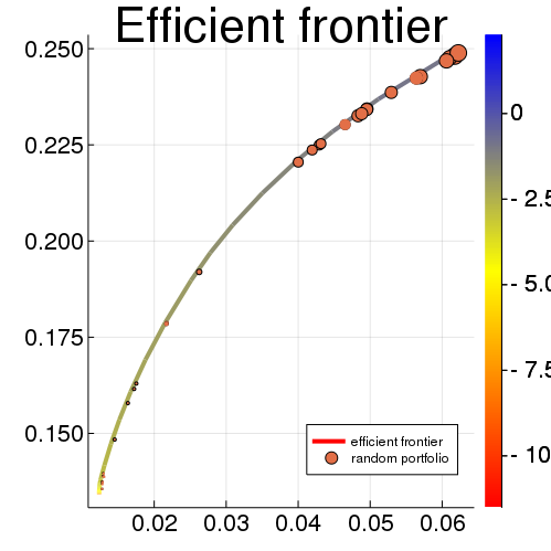
The validation consists of three steps. First, we plot the efficient frontiers (EF) by increasing $r$ in the Forward Problems. Each data point on the EF curve represents a (risk, profit) pair determined by a predefined $r$ . Smaller $r$ are positioned closer to origin points on the EF curve, whereas larger values locate far from the origin on the EF curve. Then, we uniformly sample a number of (e.g., 30) risk tolerance values along the curve from small to large, and use the optimal allocation results as inputs to solve the Inverse problems. Then, the estimated values are compared with true values. We compare both the orders and the absolute values along diagonal lines. Ideally, good estimations should align most points on the diagonal (Figure 1).

Refer to caption — Figure 1. Order Estimation of Risk Tolerance Values. The plot is generated using VFINX asset data observed from Jan 1st 2000 to March 31st 2015 aggregated to sector level. First, the efficient frontier curve in the left figure is generated by solving *forward problem* using 100 evenly sampled $r$ values on logspace from -5 to 1, corresponding to $r=[10^{-5},...,10]$ . The coordinates of curve are (Risk, Profit) values represented by ( $\mathbf{x}^{T}Q\mathbf{x},\mathbf{c}^{T}\mathbf{x}$ ) where $\mathbf{x}$ are obtained by solving Forward problem. The color of curve is mapped to the logarithm of risk tolerance values as indicated in color map. In the same log space, 30 random risk tolerance values, indicated by red circles, are sampled in uniform distributions. The sizes of circles are proportional to their values. Then, portfolios generated by these samples in *Forward Problem* are used as observations to estimate back $r$ in *inverse problem*. The right figure compares the order of true values (x-axis) with the order of estimated values (y-axis).

4.2. Time-Series Portfolios Experimental Framework

4.2.1. Time-series Portfolio Data $Y$

We define asset-level portfolio holdings $Y=\{\mathbf{y}_{1},...,\mathbf{y}_{C}\}$ collected from starting date $\delta_{y}(1)$ till ending date $\delta_{y}(C)$ , where $\delta_{y}(\cdot)$ is a function that maps portfolio data indices to dates. $Y$ may be collected at different frequencies (e.g., daily, quarterly, etc.), and each $\mathbf{y}_{t}\in Y(t=1,...,C)$ represents a portfolio vector consists of $n$ assets.

4.2.2. Asset Price Data $P$

Analogously, asset price market data $P=\{\mathbf{p}_{1},...,\mathbf{p}_{D}\}$ is usually collected using some public APIs (e.g., AlphaVantage(AlphaVantage [n.d.]), Yahoo Finance) from starting date $\delta_{p}(1)$ to ending date $\delta_{p}(D)$ . In our approach, $P$ is recorded at trading-day daily bases and the raw data includes market opening price and market closing price. On that basis, we use a 253-day rolling window (trading days) to calculate yearly profit ratios using the current day market closing price minus previous year’s market opening price, then normalized by the later to obtain an annual return sequence $P^{\prime}=\{\mathbf{p}^{\prime}_{1},...,\mathbf{p}^{\prime}_{D}\}$ . Also, we usually collect more historical price data than portfolio data, therefore $D$ is usually larger than $C$ , and $\delta_{p}(1)$ is earlier than $\delta_{y}(1)$ .

4.2.3. Align Portfolio data with Asset Price data

The collections of $Y$ and $P$ then will be aligned on the same time horizon. Lets define $t$ is an observation day, $\delta_{y}^{-1}(t)$ is a function to map $t$ to the index number in $Y$ , and $\delta_{p}^{-1}(t)$ maps $t$ to index in $P$ . Thus, after aligning, we can layout $P$ on the time horizon from $\delta_{p}(1)$ to $\delta_{p}(D)$ , and $Y$ from $\delta_{y}(1)$ to $\delta_{y}(D)$ . At a observation point $t$ (if $t$ is overlapped with portfolio and price data spans), we have observed portfolio sequence $Y_{t}=\{\mathbf{y}_{1},...,\mathbf{y}_{\delta_{y}^{-1}(t)}\}$ , and price sequence $P_{t}=\{\mathbf{p}_{1},...,\mathbf{p}_{\delta_{y}^{-1}(t)}\}$ . We treat those as historical price data and portfolio data till observation time $t$ , and use them to learn risk preference at time $t$ .

4.2.4. Look-back window and Uncertainty Measure

Usually it is an arbitrary choice to determine the starting date of price $\delta_{p}(1)$ included in analysis. Sometimes this choice could have impacts on the forward portfolio construction results as well as inverse risk preference learning. To simulate this uncertainty, we introduce a look back window $l$ as adjustment of the observation of historical market signals $P$ , given by $P_{t}=\{\mathbf{p}_{l},...,\mathbf{p}_{\delta_{y}^{-1}(t)}\}$ . When $l=1$ , we end up using all collected historical price data, and we can increase $l$ with a certain step length to $L$ . For example, if $L=100$ , it means we truncate out almost half year of collected price data, and use the remaining data as observations to learn risk preference. In our experiment, we usually try different $l$ values from 1 to $L$ , and report the mean and standard deviations of learned risk preferences.

4.2.5. Calculating time-varying covariance matrices and expected portfolio returns

At each observation time $t$ , the covariance matrix and expected return of $n$ assets $\mathbf{c}_{t}$ is calculated as

(21)		$\displaystyle Q_{t}$	$\displaystyle=\textrm{cov}([\mathbf{p}^{\prime}_{l},...,\mathbf{p}_{t}],[\mathbf{p}^{\prime}_{l},...,\mathbf{p}_{t}]),$
(22)		$\displaystyle\mathbf{c}_{t}$	$\displaystyle=[c_{1,t},...,c_{i,t},...,c_{n,t}]^{T},$

where $c_{i,t}=\textrm{mean}([p^{\prime}_{i,l},...,p^{\prime}_{i,t}])$ is the mean profit value of $i-$ th asset in historical price data.

4.2.6. Learning time-varying risk preferences

Now we can define a date range called learning period, from $T_{s}$ to $T_{e}$ from the time horizon where $P$ and $Y$ overlap. Usually we select a $T_{s}$ later than the first portfolio date $\delta_{p}(1)$ because we want to include multiple samples $\{y_{1},...,y_{\delta_{y}^{-1}(T_{s})}\}$ for online learning. Otherwise, if we set $T_{s}==\delta_{p}(1)$ , then the first observation will have only one portfolio sample, and the learned risk preferences at the beginning could be very unstable because there is not enough samples to learn. After learning at $T_{s}$ , we move to $T_{s}+1$ and include a new sample in our portfolio in observed sequence, and learn the next risk preference, and so on. If from $T_{s}$ to $T_{e}$ there are $T$ number of learning period, we obtain a time-varying risk preference curve. And with adjustments of look back window $l$ , we repeat the process can simulate a confidence band of risk preferences.

4.2.7. Aggregation of $Q_{t},Y_{t},\mathbf{c}_{t}$ :

When the sizes of portfolios are large ( $n$ >1000) such as mutual funds mentioned in Section 6, to increase the efficiency and stability of IPO ( $n=500$ takes 80 CPU seconds, $n>1000$ takes more than 1000 seconds), also to enable easy comparison of portfolios with different sizes, we may group assets by sectors, or apply PCA on $Q_{t}$ to factorize portfolios, thus obtaining $Q_{s,t},c_{s,t},y_{s,t}$ in sector space and $Q_{f,t},c_{f,t},y_{f,t}$ in factor space respectively to learn risk preferences in Sector or Factor space.

So far we have introduced a general experimental framework setup for time varying portfolio risk preference learning. In next two sections, we will use this framework to explain our data sets and experimental settings.

5. Case Study 1: Robotic portfolios

We apply proposed method on a series of actively-managed portfolios generated from an in-house portfolio construction platform. This platform utilizes a Deep Reinforcement Learning (DRL) model (Wang and Yu 2021) to automatically construct portfolios for specified target investment goals. The DRL model addresses a similar objective as the forward problem 3.1 used in our risk preference learning approach, but formulates it in multi-period setting (Li and Ng 2000) and generates auto-balanced portfolios through deep reinforcement learning. An important input parameter to specify in such a DRL model is the expected portfolio return, which could be easily proved to have a one-to-one correspondence with the risk preference in single-period mean-variance formulation (See Appendix 8.4). Since specifying target return is more intuitive to investors than determining risk preference, the DRL system relies on extensions of the following equivalent formulation:

\displaystyle\begin{array}[]{llll}\min\limits_{\mathbf{x}\in\mathbb{R}^{n}}&\frac{1}{2}\mathbf{x}^{T}Q\mathbf{x}\\ \;s.t.&\mathbf{c}^{T}\mathbf{x}=z,\\ &A\mathbf{x}\geq\mathbf{b}\end{array}

where $z$ is the expected portfolio return. In the multi-period optimization (MPO) setting (Li and Ng 2000), the dynamics of the portfolio rebalanced at time point $i=0,1,2,...,N-1$ is

\displaystyle\begin{array}[]{llll}W_{i+1}=\sum_{j=1}^{n}v_{i}^{j}\frac{S_{i+1}^{j}}{S_{i}^{j}}+W_{i}-\sum_{j=1}^{n}v_{i}^{j},\quad i=0,\dots,N-1.\end{array}

where $W_{i}$ represents the wealth at the $i$ -th fine-tuning time, $S_{i}^{j}$ represents the price of stock $j$ at $i$ . The vector $\mathbf{v}_{i}=(v_{i}^{1},v_{i}^{2},\dots,v_{i}^{n})^{T}$ gives the dollar value allocations among all the $n$ stocks in the portfolio at each fine-tuning time $i$ . The precise multi-period extension is hence

	$\displaystyle\min_{\mathbf{v}_{i},i=0,\dots,N-1}\text{Var}[W_{N}],$
(27)		$\displaystyle\;s.t.\ \mathbb{E}[W_{N}]=1+z.$

It is assumed above that the initial capital $W_{0}=1$ . Our in-house DRL platform solves the problem in equation (27) using deep neural networks and actor-critic RL methodologies. More information about the implemented DRL algorithms is available in (Wang and Yu 2021).

Experimental Setup: The DRL model is trained and validated using daily market price data of S&P 500 stocks from 2017-04-01 to 2019-04-01, and generates daily-rebalanced portfolios from 2019-04-01 till 2020-12-10. DRL allows investor to specify the size of portfolio ( $n$ assets), and also provides options allowing switching of assets or keeping the same assets. In our experiments, we turn off asset switching functions, and create three sizes of portfolios (10, 50, 100 assets) using three specified annual expected portfolio returns (10%, 20%, 30%) as investment target. The DRL model automatically rebalances the portfolios per each trading day, so for the whole test period it generated 9 different time-series portfolios (combing asset size with target profit) where each portfolio is composed by 425 daily portfolio vectors. Our goal is to learn the risk preferences of these robotic portfolios and compare our learning results with the investment target values that drive the DRL model.

Per discussions about experimental framework in Section 4.2, the portfolio starting date $\delta_{y}(1)$ is 2019-04-01, and ending date $\delta_{y}(C)$ is 2020-12-10. The price data starting date $\delta_{p}(1)$ is 2000-01-02, and ending date $\delta_{p}(D)$ is 2020-12-10. Because the portfolios are daily data, the price dates and portfolio dates are aligned on trading days. We set the observation period $T_{s}=\delta_{y}(1)$ and $T_{e}=\delta_{y}(C)$ . The look back period adjustment $l$ are ten values from $\{1,11,21,...,101\}$ . Hyper-parameters are optimized using as single point forward-backward validation (Section 4.1).

Results: Our results show that even if these robotic portfolios are constructed using a different (more complicated, across-time) objective, the proposed inverse optimization process can still learn the ordinal relationships of important decisional inputs governing the investment procedures. As shown in Figure 3, the learned daily risk preference curves corresponding to higher target returns are generally larger than those associated with lower target returns in all portfolios. Most of the time, the learned risk preferences are stable across the investment period, but significant volatility occurs on some portfolios around March 2020, which is understandable because it reflects the market movement that happened during that period. If we first look at the return of those robotic portfolios (bottom figures), all portfolios have positive returns before turning negative till March 2020, and afterward, they all recover to be profitable. Small portfolios composed of 10 assets achieve higher returns at Dec 2020 (about 100% actual profits for those targeting 30% annual returns), whereas larger portfolios have slightly lower returns (about 50% actual profits for 50-asset and 100-asset portfolios targeting 30% yearly returns). Linking the investment targets of portfolio returns back to learned risk preferences at the top figures, they are generally consistent at the ordinal level, which is also understandable because of the one-to-one correspondence between target return and risk preference in the DRL’s multi-period objective function. It is also noticeable that around March 2020 three risk preference curves vibrate drastically (10-asset target 30%, 50-asset target 20% and 100-asset target 10%), which might be due to the regime switch in DRL model because of the underlying changes of market data, as well as the rigidness of the long-only allocation constraint.

Discussions: Besides the promising results, it is also noticeable that the sizes of portfolios impact risk preferences learned by the proposed method. According to our experiments, larger portfolios usually lead to smaller risk preferences. Apart from the coincidence in portfolio theory that diversification is preferable in investment (which may imply lower risk), we believe this is more due to the numerical issue in the 3.1 objective: when the dimension of $x$ turns higher under the constraints that its L1-norm should be 1, the first quadratic term $x^{T}Qx$ becomes smaller, and thus impacts the risk preference parameter $r$ in the second term, which is basically a regularization parameter, to turn smaller. Such a property causes an issue when we compare risk preferences across portfolios of different sizes, and we will address this issue in the next case study.

6. Case Study 2: Mutual Funds

In this case study, we will explore risk preferences learning on seven time-series mutual fund portfolio holdings. To compare portfolios of different sizes, we propose two extensions of the original asset-level algorithm by aggregating high dimensional portfolios into sector space and factor space. The sector space algorithm utilizes attribute knowledge of each asset and groups them into 11 industrial sectors. Alternatively, we can apply Principal Component Analysis (or other factor analysis) on the covariance matrix and learn risk preferences on factorized portfolios. Due Readers interested in these extensions can read the detailed derivations at this paper’s full version at arXiv.

Mutual Funds: VFINX and SWPPX are S&P 500 funds broadly diversified in large-cap market. FDCAX’s portfolio mainly consists of large-cap U.S. stocks and a small number of non-U.S. stocks. VHCAX is an aggressive growth fund invests in companies of various sizes that the managers believe will grow in time but may be volatile in the short-term. VSEQX is an actively managed fund holding mid- and small-cap stocks that the advisor believes have above-average growth potential. VSTCX is also an actively managed fund that offers broad exposure to domestic small-cap stocks believed to have above-average return potential. LMPRX mainly invests in common stocks of companies that the manager believes will have current growth or potential growth exceeding the average growth rate of companies included in S&P 500.

The reasons of analyzing mutual fund portfolios are threefold. First, mutual fund holdings are freely accessible public data and it is easier to discuss and interpret results using public data than clients’ private data. Second, mutual funds are usually constructed by tracking industry capitalization indices, or managed by fund managers. Thus, they can be considered as optimal portfolios constructed through rational decision making. Moreover, risk measurements of mutual funds are common knowledge reported by several well-known metrics and estimations with our methods can be directly validated by these metrics. Third, mutual funds usually are diversified on large numbers of assets and they fit the underlying MPT used in our model. Moreover, high-dimensional portfolios are challenging to optimize in the inverse optimization problem and they really test the efficiency of our approach.

Experimental Setup: We collect 10 years of asset-level portfolio holdings of the aforementioned seven mutual funds from quarterly reports publicly available on SEC website, starting from March 2010 ( $\delta_{y}(1)$ ) to Dec 2020( $\delta_{y}(C)$ ). We also collect twenty years of historical asset level price data from July 1st, 2001 ( $\delta_{p}(1)$ ) to Dec 21st, 2020 ( $\delta_{p}(D)$ ). The learning period is set from March 2015 ( $T_{s}$ , corresponding to $\delta_{y}^{-1}(T_{s})=21$ ) till Dec 2020 ( $T_{e}$ , corresponding to $\delta_{y}^{-1}(T_{e})=44$ ). Market price data is aggregated to monthly level to align with quarterly portfolio. The adjustment parameter of look back $l$ is evenly selected from $1,3,5,...,11$ (months).

To further validate the estimated risk tolerance values, we compare them with two standard metrics evaluating investment risk used in financial domain: Inverse of Sharpe Ratio and Mutual Fund beta values .

Comparison with Inverse of Sharpe Ratio: In finance, the Sharpe ratio (Sharpe 1965) measures the performance of a portfolio compared to a risk-free asset, after adjusting the risk it bears. It is defined as the difference between the expected return of the asset return $E(R_{a})$ and the risk-free return $E(R_{f})$ , divided by the standard deviation of the investment:

(28)

\displaystyle S_{a}=\frac{E(R_{a})-E(R_{f})}{\sigma}

Note that the Sharpe ratio is proportional to risk-aversion. In our paper, we use a modified Inverse Sharpe ratio to compare with learned risk tolerance values:

(29)

\displaystyle IS_{a,t}=\frac{\mathbf{x}_{a,t}^{T}Q_{a,t}\mathbf{x}_{a,t}}{\mathbf{c}_{a,t}^{T}\mathbf{x}_{a,t}}

In (29), $\mathbf{x}_{a,t},Q_{a,t},\mathbf{c}_{a,t}$ are variables defined over asset-level, and change over time. To avoid redundant discussions, we analogously derive similar Inverse Sharpe ratios in sector and factor space.

According to Figure 4, estimated $r$ are more volatile over time in sector space, and the confidence intervals are generally wider than inverse Sharpe ratios. However, in factor space, estimated $r$ becomes smooth and Inverse Sharpe ratio is mostly lower than proposed risk preference, where the main reason is factors represent dominant volatility.

Comparison with Mutual Fund beta values: In Capital Asset Pricing Model (CAPM) (Treynor 1961; Sharpe 1964; Lintner 1969; Mossin 1966), the beta coefficient of a portfolio is a measure of the risk arising from exposure to general market movements as opposed to idiosyncratic factors, given by

(30)

\displaystyle\beta_{a}=\frac{E(R_{a})-E(R_{f})}{E(R_{m})-E(R_{f})},

where $E(R_{m})$ is the expected return of market (e.g., benchmark portfolio) and others are the same as defined in (28). The beta measures how much risk the investment is compared to the market. If a stock is riskier than the market, it will have a beta greater than one. If a stock has a beta of less than one, the formula assumes it will reduce the risk of a portfolio.

The beta values of mutual funds are public data and change over time. We list the recent two beta values in Table 1.

	VFINX	SWPPX	FDCAX	VHCAX	VSEQX	VSTCX	LMPRX
$\beta$ (2019)	1.0	1.0	1.03	1.14	1.17	1.22	1.17
$\beta$ (2020)	1.0	1.0	1.01	1.13	1.30	1.38	1.07

Table 1. Beta values of mutual funds studied in our paper

We sort the averaged risk-tolerance values of 7 mutual funds over time from small to large, and compare their orders with the order of beta values averaged from Table 1. In Figure 4 (h), most of the scatter plots are close to diagonal, indicating that the order of estimated risk tolerance is consistent with the order of beta values. Therefore, risk indicators estimated by proposed methods are intuitively rational because they are consistent with common knowledge in the financial domain.

Readiness for automated and personalized portfolio construction Our risk tolerance parameters can be directly used as inputs in the mean-variance framework to drive automated portfolio advice, known as Robo-advising. Most existing Robo-advising systems construct risk preference parameters according to one-time interaction with the client (Capponi et al. 2019), typically profiled based on client’s financial objectives, investment horizons, and demographic characteristics. Other approaches assume the client knows her risk tolerance parameter at all times, but only communicates it to the Robo-advisor at specific updating times(Capponi et al. 2019). With our approach, we could anchor investor client’s risk at an appropriate level compared to some benchmark portfolios. Our experiments show that the time-varying risk preference of two S&P 500 mutual funds, which are considered a market benchmark portfolio, range from 0.2 to 0.5 in Sector Space. We also illustrate that some actively managed funds (VSEQX, VSTCX) have larger risk preference values than 0.5. For example, if the client is aware that S&P 500 fund has risk tolerance $r=0.2$ and an active fund has risk tolerance $r=0.5$ , she may prefer to have a personalized risk tolerance that is between those of the S&P 500 fund and active fund at current market period. The Robo-advisor can directly suggest a personalized risk tolerance score $r=0.4$ and start with a personalized portfolio construction process. Later, when the market has changed, risk tolerance values of S&P 500 fund and active funds may also change accordingly. The Robo-advisor should update the process with a new parameter to reflect the time-varying risk preference.

7. Conclusions

In this paper, we present a novel approach to learn risk preference parameters from portfolio allocations. We formulate our learning task in a generalized inverse optimization framework. We consider portfolio allocations as outcomes of an optimal decision-making process governed by mean-variance portfolio theory, thus risk preference parameter is a learnable decision variable through IPO. The proposed approach has been validated and exhibited in two real problems that consists of a 18-month of daily robotic investment portfolios and ten-year history of quarterly portfolio holdings collected in seven mutual funds. The proposed method can be applied to individual investors’ portfolios to understand their risk profiles in personalized investment advice. It could be deployed as real-time reference indices in Robo-advising systems that facilitate automation and personalization.

References

(1)
Ahuja and Orlin (2001) Ravindra K Ahuja and James B Orlin. 2001. Inverse optimization. Operations Research 49, 5 (2001), 771–783.
Aït-Sahalia and Lo (2000) Yacine Aït-Sahalia and Andrew W Lo. 2000. Nonparametric risk management and implied risk aversion. Journal of Econometrics 94, 1-2 (2000), 9–51.
AlphaVantage ([n.d.]) AlphaVantage. [n.d.]. AlphaVantage API Documentation. https://www.alphavantage.co/documentation/. Accessed: 2020.
Alsabah et al. (2020) Humoud Alsabah, Agostino Capponi, Octavio Ruiz Lacedelli, and Matt Stern. 2020. Robo-Advising: Learning Investors’ Risk Preferences via Portfolio Choices*. Journal of Financial Econometrics (01 2020). https://doi.org/10.1093/jjfinec/nbz040 arXiv:https://academic.oup.com/jfec/article-pdf/doi/10.1093/jjfinec/nbz040/31700703/nbz040.pdf nbz040.
Arrow (1971) Kenneth J Arrow. 1971. The theory of risk aversion. Essays in the theory of risk-bearing (1971), 90–120.
Aswani et al. (2018) Anil Aswani, Zuo-Jun Shen, and Auyon Siddiq. 2018. Inverse optimization with noisy data. Operations Research (2018).
Bärmann et al. (2017) Andreas Bärmann, Sebastian Pokutta, and Oskar Schneider. 2017. Emulating the expert: Inverse optimization through online learning. In ICML.
Barsky et al. (1997) Robert B Barsky, F Thomas Juster, Miles S Kimball, and Matthew D Shapiro. 1997. Preference parameters and behavioral heterogeneity: An experimental approach in the health and retirement study. The Quarterly Journal of Economics 112, 2 (1997), 537–579.
Bertsimas et al. (2012) Dimitris Bertsimas, Vishal Gupta, and Ioannis Ch Paschalidis. 2012. Inverse optimization: A new perspective on the Black-Litterman model. Operations Research 60, 6 (2012), 1389–1403.
Bertsimas et al. (2015) Dimitris Bertsimas, Vishal Gupta, and Ioannis Ch Paschalidis. 2015. Data-driven estimation in equilibrium using inverse optimization. Mathematical Programming 153, 2 (2015), 595–633.
Birge et al. (2017) John R Birge, Ali Hortaçsu, and J Michael Pavlin. 2017. Inverse optimization for the recovery of market structure from market outcomes: An application to the miso electricity market. Operations Research 65, 4 (2017), 837–855.
Black and Litterman (1992) Fischer Black and Robert Litterman. 1992. Global Portfolio Optimization. Financial Analysts Journal 48, 5 (1992), 28–43. https://doi.org/10.2469/faj.v48.n5.28 arXiv:https://doi.org/10.2469/faj.v48.n5.28
Brennan and Lo (2011) Thomas J Brennan and Andrew W Lo. 2011. The origin of behavior. The Quarterly Journal of Finance 1, 01 (2011), 55–108.
Capponi et al. (2019) Agostino Capponi, Sveinn Ólafsson, and Thaleia Zariphopoulou. 2019. Personalized Robo-Advising: Enhancing Investment through Client Interactions. Wealth Management eJournal (2019).
Chan et al. (2014) Timothy CY Chan, Tim Craig, Taewoo Lee, and Michael B Sharpe. 2014. Generalized inverse multiobjective optimization with application to cancer therapy. Operations Research 62, 3 (2014), 680–695.
Chan and Kaw (2020) Timothy CY Chan and Neal Kaw. 2020. Inverse optimization for the recovery of constraint parameters. European Journal of Operational Research 282, 2 (2020), 415–427.
Chan and Lee (2018) Timothy CY Chan and Taewoo Lee. 2018. Trade-off preservation in inverse multi-objective convex optimization. European Journal of Operational Research 270, 1 (2018), 25–39.
Chan et al. (2019) Timothy CY Chan, Taewoo Lee, and Daria Terekhov. 2019. Inverse optimization: Closed-form solutions, geometry, and goodness of fit. Management Science (2019).
Chetty (2006) Raj Chetty. 2006. A new method of estimating risk aversion. American Economic Review 96, 5 (2006), 1821–1834.
Cohen and Einav (2007) Alma Cohen and Liran Einav. 2007. Estimating risk preferences from deductible choice. American economic review 97, 3 (2007), 745–788.
Cohn (1975) et al Cohn, Richard A. 1975. Individual Investor Risk Aversion and Investment Portfolio Composition. Journal of Finance 30, 2 (May 1975), 605–620. https://ideas.repec.org/a/bla/jfinan/v30y1975i2p605-20.html
Dong et al. (2018) Chaosheng Dong, Yiran Chen, and Bo Zeng. 2018. Generalized Inverse Optimization through Online Learning. In NeurIPS.
Dong and Zeng (2018) Chaosheng Dong and Bo Zeng. 2018. Inferring Parameters Through Inverse Multiobjective Optimization. arXiv preprint arXiv:1808.00935 (2018).
Dong and Zeng (2020) Chaosheng Dong and Bo Zeng. 2020. Expert Learning through Generalized Inverse Multiobjective Optimization: Models, Insights, and Algorithms. In ICML.
Esfahani et al. (2018) Peyman Mohajerin Esfahani, Soroosh Shafieezadeh-Abadeh, Grani A Hanasusanto, and Daniel Kuhn. 2018. Data-driven inverse optimization with imperfect information. Mathematical Programming 167, 1 (2018), 191–234.
Grinold and Kahn (2000) R. C. Grinold and R.N Kahn. 2000. Active Portfolio Management. McGraw-Hill, New York.
Guiso and Paiella (2008) Luigi Guiso and Monica Paiella. 2008. Risk aversion, wealth, and background risk. Journal of the European Economic association 6, 6 (2008), 1109–1150.
Hanna et al. (1998) Sherman Hanna, Michael Gutter, and Jessie Fan. 1998. A theory based measure of risk tolerance. Proceedings of the Academy of Financial Services 15 (1998), 10–21.
He and Litterman (2002) Guangliang He and Robert B. Litterman. 2002. The Intuition Behind Black-Litterman Model Portfolios.
Hey (1999) John D Hey. 1999. Estimating (risk) preference functionals using experimental methods. In Uncertain Decisions. Springer, 109–128.
Holt and Laury (2002) Charles A Holt and Susan K Laury. 2002. Risk aversion and incentive effects. American economic review 92, 5 (2002), 1644–1655.
Iyengar and Kang (2005) Garud Iyengar and Wanmo Kang. 2005. Inverse conic programming with applications. Operations Research Letters 33, 3 (2005), 319–330.
Keshavarz et al. (2011) Arezou Keshavarz, Yang Wang, and Stephen Boyd. 2011. Imputing a convex objective function. In Intelligent Control (ISIC), 2011 IEEE International Symposium on. IEEE, 613–619.
Li and Ng (2000) Duan Li and Wan-Lung Ng. 2000. Optimal Dynamic Portfolio Selection: Multiperiod Mean-Variance Formulation. Mathematical Finance 10, 3 (2000), 387–406. https://EconPapers.repec.org/RePEc:bla:mathfi:v:10:y:2000:i:3:p:387-406
Linnér (2019) Richard Karlsson et al. Linnér. 2019. Genome-wide association analyses of risk tolerance and risky behaviors in over 1 million individuals identify hundreds of loci and shared genetic influences1. bioRxiv (2019). https://doi.org/10.1101/261081 arXiv:https://www.biorxiv.org/content/early/2019/01/08/261081.full.pdf
Lintner (1969) John Lintner. 1969. The Valuation of Risk Assets and the Selection of Risky Investments in Stock Portfolios and Capital Budgets: A Reply. The Review of Economics and Statistics 51, 2 (May 1969), 222–224.
Lu and Perrigne (2008) Jingfeng Lu and Isabelle Perrigne. 2008. Estimating risk aversion from ascending and sealed-bid auctions: The case of timber auction data. Journal of Applied Econometrics 23, 7 (2008), 871–896.
Markowitz (1952) Harry Markowitz. 1952. Portfolio selection. The Journal of Finance 7, 1 (1952), 77–91.
Mcgraw et al. (2010) A. Peter Mcgraw, Jeff Larsen, and David Schkade. 2010. Comparing Gains and Losses. Psychological science 21 (10 2010), 1438–45. https://doi.org/10.1177/0956797610381504
Mossin (1966) Jan Mossin. 1966. EQUILIBRIUM IN A CAPITAL ASSET MARKET. Econometrica 34 (1966), 768.
O’Donoghue and Somerville (2018) Ted O’Donoghue and Jason Somerville. 2018. Modeling Risk Aversion in Economics. Journal of Economic Perspectives 32 (05 2018), 91–114. https://doi.org/10.1257/jep.32.2.91
Payne et al. (2017) Brian Payne, Jazmin Brown-Iannuzzi, and Jason Hannay. 2017. Economic inequality increases risk taking. Proceedings of the National Academy of Sciences 114 (04 2017), 201616453. https://doi.org/10.1073/pnas.1616453114
Post et al. (2008) Thierry Post, Martijn J Van den Assem, Guido Baltussen, and Richard H Thaler. 2008. Deal or no deal? decision making under risk in a large-payoff game show. American Economic Review 98, 1 (2008), 38–71.
Pratt (1964) John W. Pratt. 1964. Risk Aversion in the Small and in the Large. Econometrica 32, 1/2 (1964), 122–136.
Rabin and Thaler (2001) Matthew Rabin and Richard H Thaler. 2001. Anomalies: risk aversion. Journal of Economic perspectives 15, 1 (2001), 219–232.
Schaefer (2009) Andrew J. Schaefer. 2009. Inverse integer programming. Optimization Letters 3, 4 (2009), 483–489.
Schooley and Worden (1996) Diane K. Schooley and Debra Drecnik Worden. 1996. Risk Aversion Measures: Comparing Attitudes and Asset Allocation. Financial Services Review 5 (1996), 87–99.
Sharpe (1964) William Sharpe. 1964. CAPITAL ASSET PRICES: A THEORY OF MARKET EQUILIBRIUM UNDER CONDITIONS OF RISK. Journal of Finance 19, 3 (1964), 425–442. https://EconPapers.repec.org/RePEc:bla:jfinan:v:19:y:1964:i:3:p:425-442
Sharpe (1965) William Sharpe. 1965. Mutual Fund Performance. The Journal of Business 39 (1965). https://EconPapers.repec.org/RePEc:ucp:jnlbus:v:39:y:1965:p:119
Sokol-Hessner et al. (2009) Peter Sokol-Hessner, Ming Hsu, Nina G Curley, Mauricio R. Delgado, Colin F. Camerer, and Elizabeth A. Phelps. 2009. Thinking like a trader selectively reduces individuals’ loss aversion. Proceedings of the National Academy of Sciences 106 (2009), 5035 – 5040.
Szpiro (1986) George G Szpiro. 1986. Relative risk aversion around the world. Economics Letters 20, 1 (1986), 19–21.
Treynor (1961) Jack L. Treynor. 1961. Market Value, Time, and Risk.
von Neumann and Morgenstern (1947) J. von Neumann and O. Morgenstern. 1947. Theory of games and economic behavior. Princeton University Press.
Wang and Yu (2021) Haoran Wang and Shi Yu. 2021. Robo-advising: Enhancing investment with inverse optimization and deep reinforcement learning. arXiv preprint (2021).
Wang (2009) Lizhi Wang. 2009. Cutting plane algorithms for the inverse mixed integer linear programming problem. Operations Research Letters 37, 2 (2009), 114–116.

8. Supplementary Material A: Learning Risk in Sector and Factor Space

In this section, we introduce reformulations of 3.3 for sector-based and factor-based risk preference learning in details.

8.1. Sector Space

8.1.1. Forward Problem

Similar to 3.1, we consider the following mean-variance portfolio optimization problem in sector space:

\displaystyle\begin{array}[]{llll}\min\limits_{\mathbf{x}}&\frac{1}{2}\mathbf{x}_{s}^{T}Q_{s}\mathbf{x}_{s}-r_{s}\mathbf{c}_{s}^{T}\mathbf{x}_{s}\\ \;s.t.&A_{s}\mathbf{x}_{s}\geq\mathbf{b}_{s},\end{array}

where $Q_{s}$ is the sector level variance-covariance matrix, $\mathbf{x}_{s}$ is the portfolio allocation aggregated in sector space, $\mathbf{c}_{s}$ is the expected sector level portfolio return, $r_{s}$ is the risk tolerance factor (in sector space), $A_{s}$ is the structured constraint matrix, and $\mathbf{b}_{s}$ is the corresponding constraint value.

Similar to Section 4.2.5, time-varying $Q_{s,t}$ and $\mathbf{c}_{s,t}$ are defined as follows:

\displaystyle\begin{array}[]{llll}Q_{s,t}&=\textrm{cov}([\mathbf{p}_{s,l},...,\mathbf{p}_{s,t}],[\mathbf{p}_{s,l},...,\mathbf{p}_{s,t}]),\\ \mathbf{p}_{s,t}&=[\hat{p}_{i,t}]_{i\in\mathcal{S}_{i}}\\ \hat{p}_{i,t}&=\sum\limits_{j\in\mathcal{S}_{i}}w_{j,t}p_{j,t},\\ c_{i,t}&=\textrm{mean}([\hat{p}_{i,t-w},...,\hat{p}_{i,t}]),\\ \mathbf{c}_{s,t}&=\{c_{1,t},...,c_{i,t},...,c_{|\mathcal{S}|,t}\},\end{array}

where $\mathbf{p_{s,t}}$ is vector of sector-level returns, $\mathcal{S}_{i}$ is the set of assets in $i$ -sector, $w_{j,t}$ is asset holding weights belonging to $\mathcal{S}_{i}$ , and $\hat{p}_{i,t}$ is time-varying sector monthly profit calculated by weighted sum of asset level profit in that sector.

8.1.2. Inverse Problem

The online inverse problem of learning sector-level risk tolerance $r_{s}$ given $\mathbf{y}_{s,t},Q_{s,t},\mathbf{c}_{s,t}$ is formulated as

\displaystyle\begin{array}[]{llll}\min\limits_{{r}_{s},\mathbf{x}_{s}\in\Theta}&\frac{1}{2}\|{r}_{s}-r_{s,t}\|^{2}+\eta_{t}\|\mathbf{y}_{s,t}-\mathbf{x}_{s}\|^{2}\\ \;s.t.&A_{s}\mathbf{x}_{s}\geq\mathbf{b}_{s},\\ &\mathbf{u}\leq M\mathbf{z},\\ &A_{s}\mathbf{x}_{s}-\mathbf{b}_{s}\leq M(1-\mathbf{z}),\\ &Q_{s,t}\mathbf{x}_{s}-r_{s}\mathbf{c}_{s,t}-A_{s}^{T}\mathbf{u}=0,\\ &\mathbf{x}_{s}\in\mathbb{R}^{m},\mathbf{u}\in\mathbb{R}_{+}^{m},\mathbf{z}\in\{0,1\}^{m}.\end{array}

The observed portfolio $\mathbf{y}_{s,t}$ is now aggregated to sector level.

8.1.3. Sector Risk Tolerance Learning Algorithm

Algorithm 1 illustrates the process of applying online IOP to learn risk tolerance using sector level data. The number of iteration $T$ varies by observed portfolio. In the mutual fund case study, at $\mathbf{y}_{20}$ , we have 20 historical quarterly portfolios so $T=20$ . $T$ increases each quarter to $T=44$ at December 2020.

Algorithm 1 Risk Tolerance Learning from Sector Portfolio

Input: (time-series portfolio and price data) ${Y}_{t},P_{t}$
Initialization: $r_{0}$ (guess), $\lambda$ , $M$ (hyper-parameter)

1: for

t=1

T

2: receive (

Y_{t},P_{t}

)

(\mathbf{y}_{s,t},\mathbf{p}_{s,t})\leftarrow(\mathbf{y}_{t},\mathbf{p}_{t})

(Q_{s,t},\mathbf{c}_{s,t})\leftarrow\mathbf{p}_{s,t}

\eta_{t}\leftarrow\lambda t^{-1/2}

\triangleright

get updated

\eta_{t}

by decaying factor

6: Solve

r_{s,t}

as 8.1.2 in Section 8.1.2

r_{s,t+1}\leftarrow r_{s,t}

\triangleright

update new guess of

r

8: end for

Output: Estimated $r_{s}$

8.1.4. Hyper-parameter and constraints

Solving the inverse problem in 8.1.2 requires hyper-parameters $M$ and $\eta_{t}$ . The constraints $A_{s}\mathbf{x}_{s}\geq\mathbf{b}_{s}$ correspond to

(44)			$\displaystyle 0\leq x_{i}\leq 1,\ \ i\in[11],$
(45)			$\displaystyle\sum_{i=1}^{11}x_{i}=1,$

as we do not consider short-selling positions. Specifically, the structural constraint coefficient matrix $A_{s}$ is a $22\times 11$ matrix, and $\mathbf{b}_{s}$ is a $22\times 1$ vector:

(46)

\displaystyle A_{s}=\begin{bmatrix}1&&&&\\ &1&&&\\ &&\ddots&&\\ &&&1&\\ &&&&1\\ -1&&&&\\ &-1&&&\\ &&\ddots&&\\ &&&-1&\\ &&&&-1\\ 1&1&\ldots&&1\\ -1&-1&\ldots&&-1\\ \end{bmatrix},\ \

\displaystyle\mathbf{b}_{s}=\begin{bmatrix}0\\ 0\\ \vdots\\ 0\\ 0\\ -1\\ -1\\ \vdots\\ -1\\ -1\\ 1\\ -1\end{bmatrix}.

8.2. Factor Space

8.2.1. Forward Problem

Without abuse of notation, we refer to the asset-level covariance matrix as $Q$ , and the asset-level return as $\mathbf{c}$ . We perform eigendecomposition of the asset-level covariance matrix $Q$ such that

(47)

\displaystyle Q\approx F\Sigma F^{T},

where $\Sigma$ is a $K\times K$ diagonal matrix of largest $K$ eigenvalues, $F$ is a $N\times K$ matrix of eigenvectors. The relationships between asset-level allocation $\mathbf{x}$ and factor-level allocation $\mathbf{x}_{f}$ are:

(48)		$\displaystyle F^{T}\mathbf{x}=\mathbf{x}_{f},$
(49)		$\displaystyle F^{T}\mathbf{c}=\mathbf{c}_{f},$

where (48) is projecting asset allocations to factor space, and (49) follows because $\mathbf{x}_{f}$ is a linear combinations of allocations in $\mathbf{x}$ , thus the expectation of returns follows the same linear combination $E[\mu_{i}x_{i}]=\mu_{i}E[x_{i}]$ .

Proposition 8.1.

The forward problem in factor space is

\displaystyle\begin{array}[]{llll}\min\limits_{\mathbf{x}_{f}}&\ \frac{1}{2}\mathbf{x}_{f}^{T}\Sigma\mathbf{x}_{f}-r_{f}\mathbf{c}_{f}^{T}\mathbf{x}_{f}\\ \;s.t.&AF\mathbf{x}_{f}\geq\mathbf{b},\end{array}

where $\mathbf{c}_{f}=F^{T}\mathbf{c}$ .

Proof.

Applying (47) and (49) to the objective function in the first term of 3.1 yields

\displaystyle\begin{array}[]{llll}&\frac{1}{2}\mathbf{x}^{T}Q\mathbf{x}\\ =&\frac{1}{2}\mathbf{x}^{T}F\Sigma F^{T}\mathbf{x}\\ =&\frac{1}{2}\mathbf{x}_{f}^{T}\Sigma\mathbf{x}_{f},\end{array}

Then, for the new projected portfolio $\mathbf{x}_{f}$ , the second term of 3.1 can be rewritten as the new term $r_{f}\mathbf{c}_{f}^{T}\mathbf{x}_{f}$ . Notice that,

\displaystyle\begin{array}[]{llll}&r_{f}\mathbf{c}_{f}^{T}\mathbf{x}_{f}\\ =&r_{f}(F^{T}\mathbf{c})^{T}F^{T}\mathbf{x}\\ =&r_{f}c^{T}FF^{T}\mathbf{x},\end{array}

where $FF^{T}$ is an Identity matrix only when $F$ contains all the eigenvectors ( $K=N$ ), and then the new objective in 8.1 is equivalent to 3.1 and $r_{f}$ is the same as $r$ . However, if $K<N$ , $FF^{T}$ is not identity matrix, so $r_{f}$ is also an approximation of $r$ in factor space. ∎

In our experiments, $Q$ is a 2236 $\times$ 2236 covariance matrix of all underlying assets included in seven mutual funds. All mutual fund holdings are represented by dimensional vector $\mathbf{y}$ , where non-holding assets are 0. The number of factors K in all our experiments is set to 5.

8.2.2. Inverse Problem

The structure of the inverse optimization problem in factor space is similar to that in asset space and sector space, and the main difference occurs on the constraint matrix $AF$ . Since $Q$ changes over time, the decomposed $\Sigma$ and $F$ also are variables depending on $t$ .

Theorem 8.2.

The inverse optimization problem in factor space is

\displaystyle\begin{array}[]{llll}\min\limits_{r_{f},\mathbf{x}_{f}\in\Theta}&\frac{1}{2}\|{r}_{f}-r_{f,t}\|^{2}+\eta_{t}\|\mathbf{y}_{f,t}-\mathbf{x}_{f}\|^{2}\\ \;s.t.&AF_{t}\mathbf{x}\geq\mathbf{b}_{f},\\ &\mathbf{u}\leq M\mathbf{z},\\ &AF_{t}\mathbf{x}_{f}-\mathbf{b}_{f}\leq M(1-\mathbf{z}),\\ &\Sigma_{t}\mathbf{x}_{f}-r_{f}\mathbf{c}_{f,t}-(AF_{t})^{T}\mathbf{u}=0,\\ &\mathbf{c}_{f,t}\in\mathbb{R}^{K},\mathbf{x}_{f}\in\mathbb{R}^{K},\mathbf{u}\in\mathbb{R}_{+}^{K},\mathbf{z}\in\{0,1\}^{K}.\end{array}

Proof.

The theorem is a direct result of applying Proposition 8.1 and KKT conditions. ∎

Remark 8.1.

The new constraint matrix $AF_{t}$ in 8.2 is no longer a sparse structural matrix as it had in 2. $AF_{t}$ now becomes a dense matrix:

(64)

\displaystyle AF_{t}=\begin{bmatrix}F_{t}^{T}\\ -F_{t}^{T}\\ \sum_{j=1}^{n}f_{j,t}\\ -\sum_{j=1}^{n}f_{j,t}\\ \end{bmatrix},\ \

\displaystyle\mathbf{b}_{f}=\begin{bmatrix}\varepsilon{\mathbf{1}}\\ -{\mathbf{1}}\\ 1\\ -1\end{bmatrix}.

where $F_{t}$ is the $N\times K$ eigenvector matrix obtained in (47), and $f_{j,t}$ are its $j$ -th column. Notice that the first vector in $\mathbf{b}_{f}$ has changed from vector of all zeros to a vector of constant value $\varepsilon$ . The reason is that solving 8.2 with a dense constraint matrix $AF_{t}$ is very challenging, and the linear equations in $AF_{t}$ can pose conflicting constraints and cause the problem infeasible. In practice, we find that relaxing one side of constraints from $0\leq AF_{t}\mathbf{x}\leq 1$ to $\varepsilon\leq AF_{t}\mathbf{x}\leq 1$ , where $\varepsilon$ is a small positive constant, can make the problem much easier to solve. Under this factor space setting, the allocation weights $\mathbf{x}_{f}$ on factors can be positive or negative values whose absolute values are larger than 1. When re-projecting them to the original asset space $F_{t}\mathbf{x}_{f}$ as (49), however, all weights are still between $\varepsilon$ and 1, and their sum is equal to 1.

8.2.3. Hyper-parameter and constraints

Solving factor space inverse problem requires three hyper-parameters: $M$ , $\lambda$ and $\varepsilon$ . The number of eigenfactor $K$ , in our paper, is set to 5 in all experiments. For dense constraint matrix $AF_{t}$ , selecting larger $K$ can make the problem very computational challenging, hence not recommended. But, if the factor coefficients assigned on asset level are sparse and consequently the constraint matrix $AF_{t}$ is also sparse, the proposed method can still learn from large number of factors efficiently.

8.2.4. Factor Risk Tolerance Learning Algorithm

The learning algorithm in factor space is illustrated in Algorithm 2. In sector space each mutual fund has different sector-based holdings, so $Q_{s,t},\mathbf{c}_{s,t}$ care calculated separately for each mutual fund. In factor space, at each observation point $t$ , $Q_{a,t},c_{a,t},F_{t},\Sigma_{t}$ are the same for all mutual funds, and $\mathbf{c}_{f,t}$ and $\mathbf{y}_{f,t}$ are different inputs from funds.

Algorithm 2 Risk Tolerance Learning from Factor Portfolio

Input: (time-series portfolio and price data) $Y_{t},P_{t}$
Initialization: $r_{0}$ (guess), $\lambda$ , $M$ , $\varepsilon$ (hyper-para)

1: for

t=1

T

2: receive (

Y_{t},P_{t}

)

(Q_{a,t},\mathbf{c}_{a,t})\leftarrow\mathbf{p}_{a,t}

(F_{t},\Sigma_{t})\leftarrow Q_{a,t}

\triangleright

eigendecomposition

(\mathbf{c}_{f,t})\leftarrow F_{t}^{T}\mathbf{c}_{a,t}

(\mathbf{y}_{f,t})\leftarrow F_{t}^{T}\mathbf{y}_{a,t}

\eta_{t}\leftarrow\lambda t^{-1/2}

\triangleright

get updated

\eta_{t}

by decaying factor

8: Solve

r_{f,t}

as equation 8.2 in Section 8.2.2

r_{f,t+1}\leftarrow r_{f,t}

\triangleright

update guess of

r_{f}

10: end for

Output: Estimated $r_{f}$

	Sector Space	Factor Space
Forward Problem	$\begin{aligned} \begin{array}[]{llll}\min\limits_{\mathbf{x}}&\frac{1}{2}\mathbf{x}_{s}^{T}Q_{s}\mathbf{x}_{s}-r_{s}\mathbf{c}_{s}^{T}\mathbf{x}_{s}\\ \;s.t.&A_{s}\mathbf{x}_{s}\geq\mathbf{b}_{s},\end{array}\end{aligned}$	$\begin{aligned} \begin{array}[]{llll}\min\limits_{\mathbf{x}_{f}}&\ \frac{1}{2}(\mathbf{x}_{f}^{T}\Sigma\mathbf{x}_{f}+\mathbf{x}_{a}^{T}Q_{d}\mathbf{x}_{a})-r_{f}\mathbf{c}_{f}^{T}\mathbf{x}_{f}\\ \;s.t.&AF\mathbf{x}_{f}\geq\mathbf{b}_{f},\end{array}\end{aligned}$
Inverse problem	$\begin{aligned} \begin{array}[]{llll}\min\limits_{{r}_{s},\mathbf{x}_{s}}&\frac{1}{2}\\|{r}_{s}-r_{s,t}\\|^{2}+\frac{\lambda}{\sqrt{t}}\\|\mathbf{y}_{s,t}-\mathbf{x}_{s}\\|^{2}\\ \;s.t.&A_{s}\mathbf{x}_{s}\geq\mathbf{b}_{s},\\ &\mathbf{u}\leq M\mathbf{z},\\ &A_{s}\mathbf{x}_{s}-\mathbf{b}_{s}\leq M(1-\mathbf{z}),\\ &Q_{s,t}\mathbf{x}_{s}-r_{s}\mathbf{c}_{s,t}-A_{s}^{T}\mathbf{u}=0,\\ &\mathbf{x}_{s}\in\mathbb{R}^{m},\mathbf{u}\in\mathbb{R}_{+}^{m},\mathbf{z}\in\{0,1\}^{m}.\end{array}\end{aligned}$	$\begin{aligned} \begin{array}[]{llll}\min\limits_{r_{f},\mathbf{x}_{f}}&\frac{1}{2}\\|{r}_{f}-r_{f,t}\\|^{2}+\frac{\lambda}{\sqrt{t}}\\|\mathbf{y}_{f,t}-\mathbf{x}_{f}\\|^{2}\\ \;s.t.&AF_{t}\mathbf{x}\geq\mathbf{b}_{f},\\ &\mathbf{u}\leq M\mathbf{z},\\ &AF_{t}\mathbf{x}_{f}-\mathbf{b}_{f}\leq M(1-\mathbf{z}),\\ &\Sigma_{t}\mathbf{x}_{f}-r_{f}\mathbf{c}_{f,t}-(AF_{t})^{T}\mathbf{u}=0,\\ &\mathbf{c}_{f,t}\in\mathbb{R}^{K},\mathbf{x}_{f}\in\mathbb{R}^{K},\mathbf{u}\in\mathbb{R}_{+}^{K},\mathbf{z}\in\{0,1\}^{K}.\end{array}\end{aligned}$
Constraints	$\begin{aligned} A_{s}=\begin{bmatrix}I\\ -I\\ \mathbf{1}\\ -\mathbf{1}\\ \end{bmatrix},\ \ &\mathbf{b}_{s}=\begin{bmatrix}\mathbf{0}\\ -\mathbf{1}\\ 1\\ -1\end{bmatrix}.\end{aligned}$	$\begin{aligned} AF_{t}=\begin{bmatrix}F_{t}^{T}\\ -F_{t}^{T}\\ \sum_{j=1}^{n}f_{j,t}\\ -\sum_{j=1}^{n}f_{j,t}\\ \end{bmatrix},\ \ &\mathbf{b}_{f}=\begin{bmatrix}\varepsilon{\mathbf{1}}\\ -{\mathbf{1}}\\ 1\\ -1\end{bmatrix}.\end{aligned}$
Hyper-parameters	$\lambda,M$	$\lambda,M,\varepsilon$

Table 2. Problem settings of risk preference learning in Sector and Factor Space.

8.3. IPO in Sector Space and Factor Space

In Table 2 we highlight the formulations of forward problem and inverse problem for IPO in sector space and factor space.

8.4. Equivalence of Mean-Variance Portfolio Problem Formulations

In mean-variance theory, the risk-tolerance parameter and the expected portfolio return parameter are closely connected and both can be used independently to trace out the mean-variance efficient frontier. Indeed, in the unconstrained scenario, the solution to the mean-variance problem

(65)

\min\limits_{\mathbf{x}\in\mathbb{R}^{n}}\frac{1}{2}\mathbf{x}^{T}Q\mathbf{x}-r\mathbf{c}^{T}\mathbf{x}

can be derived by matrix differentiation, i.e., the optimal allocation weights satisfy

Q\mathbf{x}-r\mathbf{c}=0,

which in turns gives $\mathbf{x}^{*}=rQ^{-1}\mathbf{c}$ , assuming that $Q$ is invertible. It hence follows that the targeted return $z$ satisfies

(66)

z=\mathbf{c}^{T}\mathbf{x}=r\mathbf{c}^{T}Q^{-1}\mathbf{c}.

The solution $\mathbf{x}^{*}$ to (65) can be actually recovered by solving the following equivalent mean-variance problem

\displaystyle\begin{array}[]{llll}\min\limits_{\mathbf{x}\in\mathbb{R}^{n}}&\frac{1}{2}\mathbf{x}^{T}Q\mathbf{x}\\ \;s.t.&\mathbf{c}^{T}\mathbf{x}=z.\end{array}

It is obvious from (66) that there is a one-to-one correspondence between risk aversion / tolerance parameter and the targeted return level $z$ . Moreover, equation (66) exhibits a positive relationship between risk tolerance and targeted return level. Such a positive correlation has been observed for other variants of the mean-variance problem with constraints or in the multi-period setting (see, e.g., (Grinold and Kahn 2000), (Li and Ng 2000)).

8.5. Order of 11 Sectors and Example Portfolios

We show the order of 11 sectors and the aggregated portfolios of all mutual funds at March 2020 in Table 3.

Sector Name	VFINX	SWPPX	FDCAX	VHCAX	VSEQX	VSTCX	LMPRX
Basic Materials	2.0585	2.0696	1.8866	0.00017	2.7600	3.3926	0.5647
Communication Services	10.6418	10.6255	9.6793	3.7649	3.3698	2.1419	25.7736
Consumer Cyclical	9.5455	9.4568	11.0045	8.5593	11.1654	8.2437	0.2692
Consumer Defensive	8.0814	8.0692	4.6294	0.0489	3.2521	3.5085	-
Energy	2.6315	2.6254	1.5087	1.3174	1.7545	1.9985	0.6166
Financial Services	13.8400	13.8892	9.6072	7.2355	13.2327	15.3046	0.9835
Healthcare	15.1290	15.0931	14.9797	33.7680	14.0414	14.0102	32.0470
Industrials	8.0863	8.0675	2.1276	10.4407	14.7876	14.7677	4.6743
Real Estate	2.9809	2.9807	3.1544	0	8.0989	8.0817	-
Technology	21.4863	21.4337	27.1432	27.9279	18.2084	13.3433	29.4258
Utilities	3.5461	3.5375	0.9650	0	4.8055	3.8035	-

Table 3. Sector level holdings (percentage) of Mutual Funds reported by March 2020

8.6. Computational Efficiency

Comparison of computational time solving a single iteration of 8.1.2 or 8.2. Each CPU time value shown in the table is the average number of 10 iterations consist of randomly sampled matrices. The performance is evaluated on a workstation equipped with AMD Ryzen Threadripper 1950X 16-Core and 64G memory. Notice that in reality we don’t have 500 sectors, but the complexity of solving a 500 sector problem is the same as solving a formulation of 500 asset problem, so we mainly compare asset/sector based formulation vs. factor based formulation.

Formulation	Problem Size	CPU-time(seconds)
Sector IPO	100 sectors	0.466
	200 sectors	5.908
	300 sectors	32.396
	400 sectors	46.380
	500 sectors	79.485
Factor IPO	400 assets 5 factors	3.524
	400 assets 6 factors	23.429
	400 assets 7 factors	166.250
	400 assets 8 factors	283.050
	400 assets 9 factors	293.150
	400 assets 10 factors	297.826
	500 assets 5 factors	7.365
	500 assets 6 factors	40.524
	500 assets 7 factors	221.100
	500 assets 8 factors	228.550
	500 assets 9 factors	300.350
	500 assets 10 factors	300.672

Table 4. CPU times of IPO algorithms with different sizes

Learning Risk Preferences from Investment Portfolios Using Inverse Optimization

Abstract.

Keywords:

1. Introduction

2. Related Work

3. Problem Setting

3.1. Portfolio Optimization Problem

3.2. Inverse Optimization through Online Learning

3.3. Learning Time Varying Risk Preferences

Proposition 3.1.

Proof.

Proposition 3.2.

4. Validation and Experimental Setup

4.1. Forward-Inverse Validation

4.1.1. Point Estimation

4.1.2. Ordered Risk Preference Learning

4.2. Time-Series Portfolios Experimental Framework

4.2.1. Time-series Portfolio Data YY

4.2.2. Asset Price Data PP

4.2.3. Align Portfolio data with Asset Price data

4.2.4. Look-back window and Uncertainty Measure

4.2.5. Calculating time-varying covariance matrices and expected portfolio returns

4.2.6. Learning time-varying risk preferences

4.2.7. Aggregation of Qt,Yt,𝐜tQ_{t},Y_{t},\mathbf{c}_{t}:

5. Case Study 1: Robotic portfolios

6. Case Study 2: Mutual Funds

7. Conclusions

References

8. Supplementary Material A: Learning Risk in Sector and Factor Space

8.1. Sector Space

8.1.1. Forward Problem

8.1.2. Inverse Problem

8.1.3. Sector Risk Tolerance Learning Algorithm

8.1.4. Hyper-parameter and constraints

8.2. Factor Space

8.2.1. Forward Problem

Proposition 8.1.

Proof.

8.2.2. Inverse Problem

Theorem 8.2.

Proof.

Remark 8.1.

8.2.3. Hyper-parameter and constraints

8.2.4. Factor Risk Tolerance Learning Algorithm

8.3. IPO in Sector Space and Factor Space

8.4. Equivalence of Mean-Variance Portfolio Problem Formulations

8.5. Order of 11 Sectors and Example Portfolios

8.6. Computational Efficiency

4.2.1. Time-series Portfolio Data $Y$

4.2.2. Asset Price Data $P$

4.2.7. Aggregation of $Q_{t},Y_{t},\mathbf{c}_{t}$ :