∎
Mining and Modeling Complex Leadership-Followership Dynamics of Movement dataJournal: Social Network Analysis and Mining
Abstract
Leadership and followership are essential parts of collective decision and organization in social animals, including humans. In nature, relationships of leaders and followers are dynamic and vary with context or temporal factors. Understanding dynamics of leadership and followership, such as how leaders and followers change, emerge, or converge, allows scientists to gain more insight into group decision-making and collective behavior in general. However, given only data of individual activities, it is challenging to infer the dynamics of leaders and followers. In this paper, we focus on mining and modeling frequent patterns of leading and following. We formalize new computational problems and propose a framework that can be used to address several questions regarding group movement. We use the leadership inference framework, mFLICA, to infer the time series of leaders and their factions from movement datasets, then propose an approach to mine and model frequent patterns of both leadership and followership dynamics. We evaluate our framework performance by using several simulated datasets, as well as the real-world dataset of baboon movement to demonstrate the applications of our framework. These are novel computational problems and, to the best of our knowledge, there are no existing comparable methods to address them. Thus, we modify and extend an existing leadership inference framework to provide a non-trivial baseline for comparison. Our framework performs better than this baseline in all datasets. Our framework opens the opportunities for scientists to generate testable scientific hypotheses about the dynamics of leadership in movement data.
Keywords:
Leadership followership Coordination Time Series Collective behavior1 Introduction
Leadership is a process that leaders influence followers’ actions in order to achieve the collective goal Hogg 2001; Glowacki and von Rueden 2015. Leadership is an essential part that fosters success of coordinated behaviors in social species Glowacki and von Rueden 2015; Couzin et al. 2005; Hogg 2001, such as foraging, migration, territorial defense, and so on. In most species, leadership is not permanent but may change with context (the one who leads the group to food or water may be different from the one who leads the flight from a predator) or other social circumstances (two rivaling subgroups may come to a joint decision and merge under single leadership or, vice versa, a group may split to explore several directions). Understanding dynamics of leadership, such as how leaders change, emerge, or converge, allows scientists to gain more insight into group decision-making and collective behavior in general. In this paper, we focus on mining and modeling frequent patterns of leadership dynamics.
One of the intuitive definitions of leadership that is commonly found in nature is the initiation of coordinated activities Krause et al. 2000; Smith et al. 2015; Stueckle and Zinner 2008. In the context of movement, leaders are initiators who initiate coordinated movement that everyone follows Amornbunchornvej and Berger-Wolf 2018a. There are several works have been developed to infer leaders from time series of movement data, such as FLOCK method Andersson et al. 2008, LPD framework Kjargaard et al. 2013, and methods based on a dynamic following network concept Amornbunchornvej et al. 2018 and Amornbunchornvej and Berger-Wolf 2018a.
Nevertheless, the challenges in the field still remain regarding how to infer and model the dynamics of the frequent patterns of leadership events. For example, suppose and lead separate sub-groups, how often do the two groups merge to a larger group lead by ? How likely is it that the group lead by will split into more than three sub-groups?
However, only the state-of-the-art approach, mFLICA Amornbunchornvej and Berger-Wolf 2018a, is capable of inferring dynamics of leadership – i.e. emergence, convergence, or a change of leaders – during coordinated movement. mFLICA detects clusters (factions) based on the concept of following relations. In mFLCIA, the time series from the same faction must follow the same leader.
| Properties\Frameworks | MONIC | TRACLUS,TCMM | mFLICA |
|---|---|---|---|
| Cluster types | Static clusters | Temporal clusters | Factions |
| Members of clusters | Data points | Time series | Time series |
| Tracking clusters dynamics | Yes | No | Yes |
| Following relations | No | No | Yes |
There are many works focusing on inferring dynamics of groups or clusters Li et al. 2010; Lee et al. 2007; Spiliopoulou et al. 2006. The work by Spiliopoulou et al. 2006 proposed a framework named “MONIC” to track various types of clusters transition in time series, such as expanding, splitting, merging, etc. However, MONIC infers clusters based on time points without considering following relations among time series to detect clusters. The work by Li et al. 2010; Lee et al. 2007 proposed frameworks (TRACLUS and TCMM) to detect temporal clusters from segments of time series. Nevertheless, the temporal clusters are measured based on trajectory similarity without the following relation property. Hence, MONIC, TRACLUS, and TCMM frameworks cannot be used to detect factions of time series, which implies that they cannot detect leadership and followership dynamics. Table 1 summarizes the comparison of these frameworks.
In this paper, we focus on mining frequent patterns of leadership dynamics that requires our framework to identify both groups and leaders of those groups that change over time. Moreover, since the groups following a leader during coordination have a special structure of following relations among members, the standard clustering methods cannot be used in this case.
Mining Patterns of Leadership Dynamics: Given time series of individual activities, the goal is to mine and model frequent patterns of leadership dynamics, including emergence of multiple leaders, convergence of multiple leaders to a single one, or change of a leader.
1.1 Previous contributions: leadership dynamics
To address these computational questions, in the previous paper in Amornbunchornvej and Berger-Wolf 2018b, we formalize the problem of Mining Patterns of Leadership Dynamics, as well as propose a framework, which is the extension of mFLICA Amornbunchornvej and Berger-Wolf 2018a, as a solution to this problem. We adapt the traditional framework of frequent pattern mining Agrawal et al. 1993; Han et al. 2007; Aggarwal and Han 2014 and the Hidden Markov Model (HMM) approach Rabiner 1989 to model the dynamics of frequent patterns of leadership. Our framework is capable of:
-
Mining and modeling frequent patterns of leadership dynamics : inferring the transition diagram of frequent dynamics of complex leadership events, such as “a single group lead by splits into two groups lead by and ”. In addition, we infer the probabilities of the transitions between such two events in the diagram.
-
Evaluating the significance of leadership-event order: we propose a null model of the dynamics of leadership events and perform hypothesis testing to compare frequent-pattern model of leadership dynamics inferred from the given input to our proposed null model.
-
Mining sequence patterns of leadership dynamics: finding support values for the leadership-dynamics sequences from time series of movement data.
-
Evaluating the significance of frequencies of leadership event sequences: we propose a null model of the sequences of leadership events and perform hypothesis testing to compare the support distribution of leadership event sequences inferred from the given input to our proposed null model.
We use several simulated datasets from the work in Amornbunchornvej and Berger-Wolf 2018a that cover various types of leadership dynamics for validation, as well as a dataset of trajectories of baboons Crofoot et al. 2015; Strandburg-Peshkin et al. 2015 to demonstrate the application of our framework. To the best of our knowledge, this is the first work to deal with the topic of complex leadership dynamics and there is no comparable method, therefore, we indirectly compare our framework to an enhanced FLOCK method Andersson et al. 2008, used as a baseline for leadership inference only.
1.2 New contributions: followership dynamics
While our previous work in Amornbunchornvej and Berger-Wolf 2018b addressed several aspects of leadership dynamics, there are still gaps remaining in our understanding of followership dynamics. For instance, assuming individuals and are in the same sub-group, how likely is it that they will be in different groups in the future? How many clusters of individuals are there such that members in each cluster stay together with a support at least 0.7? How likely is it for an individual that its sub-group will be lead by an individual from the same group?
Mining Patterns of Followership Dynamics: Given the time series of individual activities, the goal is to mine and model frequent patterns of followership dynamics, including the change of sub-groups of followers (unity), or the choice of whom to follow (loyalty).
To address these questions, in this paper, we extend our framework to include several aspects of followership dynamics. In addition to the previous work in Amornbunchornvej and Berger-Wolf 2018b, our framework is capable of:
-
Mining and modeling frequent patterns of faction membership: estimating the frequency of a pair of individuals being in the same faction, as well as discovering faction clusters of individuals.
-
Mining and modeling frequent patterns of leader-follower relationship: estimating the frequency of each individual being a follower of a group lead by a specific individual, as well as discovering dynamics of the changes of a leader of each faction cluster.
We also use simulated datasets from the work in Amornbunchornvej and Berger-Wolf 2018a that contain complex leader-follower dynamics to evaluate our framework. Our approach is flexible to be generalized beyond the time series of movement data to arbitrary time series where subsets intentionally or spontaneously coordinate.
2 Problem statement
In this paper, we use leadership definitions from the work in Amornbunchornvej and Berger-Wolf 2018a. Given a -dimensional time series , we use to refer to an element of the time series at time and, for a given , as a time-shifted version of where, .
Definition 1 (-Following relation (Amornbunchornvej and Berger-Wolf 2018a))
Let be a set of time series, be a time series similarity function, and be a similarity threshold. For any , we say that follows if and are sufficiently similar within some time shift :
Typically, to measure the following relation in Def. 1, the work by Amornbunchornvej and Berger-Wolf 2018a used the Dynamic Time Warping (DTW) developed by Sakoe and Chiba 1978. DTW is used to measure a distance between two time series. It can measure a distance of multi-dimensional time series (Keogh and Ratanamahatana 2005). Since DTW uses Euclidean distance as a kernel to measure a distance between a pair of elements of two time series, the weighted Euclidean distance can be deployed in the case that we want to give some dimensions higher contribution to a distance measure. Additionally, DTW performs better than several methods (Kjargaard et al. 2013) and robust to the noise ( Shokoohi-Yekta et al. 2015) for the task of following relation inference (Amornbunchornvej et al. 2018). The following relation measure using DTW is bounded in interval (Eq. 2). In the case that is not bounded, then we need a threshold to normalize the similarity measure. If , then the similarity value is one, otherwise zero.
Definition 2 (Following network (Amornbunchornvej and Berger-Wolf 2018a))
Let be a set of time series. A digraph is a following network of where each node in corresponds to a time series in and if follows .
Definition 3 (Initiator of faction (Amornbunchornvej and Berger-Wolf 2018a))
Let be a following network. is an initiator of faction if the out-degree of is zero and the in-degree of is greater than zero. The member nodes of are any nodes that have a directed path in to .
2.1 Leadership dynamics
We create a dynamic following network by considering each temporal sub-interval of of length (time window parameter) and creating a following network of that interval. We then define the notion of the time series of leaders of a dynamic following network below.
Definition 4 (Time series of leaders)
Let be a set of time series. is a time series of leaders where is a set of faction initiators at time in .
We can use mFLICA framework Amornbunchornvej and Berger-Wolf 2018a to extract a time series of leaders from time series of movement. Next, we define the support of a leader set . Let be the length of the time series of leaders and be an indicator function, which is if the statement is true, and otherwise.
| (1) |
indicates the support of having a particular set of initiators lead multiple groups concurrently. For example, if it means that half the time the leaders are exactly , leading their factions concurrently.
Definition 5 (Frequent-leader set)
Let be a time series of leaders, be a set of faction initiators, and be a support threshold. is a frequent-leader set of if .
Definition 6 (Transition probability of leader sets)
Let be a time series of leaders, and be sets of faction initiators. A transition probability of leader sets is a probability that and .
Now, we are ready to formally state the the problem of Mining Patterns of Leadership Dynamics.
In this paper, we choose to represent a set of frequent-leader sets as a diagram of leadership dynamics below.
Definition 7 (A diagram of leadership dynamics)
Let be a time series of leaders, be a support threshold, and be set of frequent-leader sets. A digraph is a diagram of leadership dynamics such that the nodes represent frequent-leader sets and if .
2.2 Followership dynamics
Given a dynamic following network of a set of time series , we define the notion of the time series of factions of the dynamic following network below.
Definition 8 (Time series of factions)
Let be a set of time series and be a dynamic following network of , where is a following network at time . We say that is a time series of factions, where is a set of factions at time in and is a set of faction members of initiator (Def. 3).
The time series of factions contains the information of who belongs to which specific faction over time. Having defined the time series of factions, we can formalize the concept of a pair of individuals who frequently stay together in the same faction.
Definition 9 (frequent co-faction pair)
Let be a time series of factions, be a threshold, and be a set of individual indices. We say that individuals and in are a frequent co-faction pair if the frequency of and being in the same faction of is greater than .
A frequent co-faction pair might indicate friendship or other strong affiliation between individuals. At the group level, we define the notion of a frequent co-faction cluster below.
Definition 10 (frequent co-faction cluster)
Let be a time series of factions, be a threshold, and be a set of individual indices. We say that a set is a frequent co-faction cluster if every member pair in is a frequent co-faction pair with respect to and and there is no other frequent co-faction cluster where . In other words, is a maximal set of frequent co-faction pairs.
A frequent co-faction cluster represents a concept of cohesion. If an entire group has a strong level of cohesion, then there are a few clusters. In contrast, if a group has a weak level of cohesion, then there are multiple clusters. The members within the same cluster might either be loyal to a specific leader, share the same interests, or be a group of friends or other strong affiliates.
In general, given a time series of factions as an input, the problem of finding global faction clusters of individuals is NP-hard, and an approximated solution was given by Tantipathananandh et al. 2007. However, in our setting, a faction or cluster is a group of followers lead by a particular frequent leader. Hence, the problem of finding global faction clusters reduces to the problem of finding followers of each frequent leader, which can be done in polynomial time in one scan over the time series.
To illustrate the concept of loyalty of a follower toward a specific leader, we formalize the notion of a frequent leader-follower pair below.
Definition 11 (frequent leader-follower pair)
Let be a time series of factions, be a threshold, and be a set of individual indices. We define the order pair () in is the frequent leader-follower pair if the frequency of having within a faction that has as the initiator with respect to is greater than .
A frequent leader-follower pair implies that is a member of a faction lead by most of the time. This implies that might be a loyal follower of (or have a strong affiliation with a loyal follower of ).
Now, we are ready to formally state the the problem of Mining Patterns of Followership Dynamics.
In this paper, we choose to represent a set of frequent co-faction pairs as a co-faction network, as well as choose to represent a set of frequent leader-follower pairs as a lead-follow network below.
Definition 12 (A co-faction network)
Let be a time series of factions, be a threshold, and be a set of individual indices. An undirected graph is a co-faction network such that there is an edge if a pair is a frequent co-faction pair w.r.t. and . The weight of the edge is a frequency of having in the same faction.
Definition 13 (A lead-follow network)
Let be a time series of factions, be a threshold, and be a set of individual indices. A bipartite graph is a lead-follow network where represents a set of follower nodes, and represents a set of initiator nodes. For any and , there is a directed edge if an order pair is a frequent leader-follower pair w.r.t. and .
3 Methods
3.1 Leadership dynamics
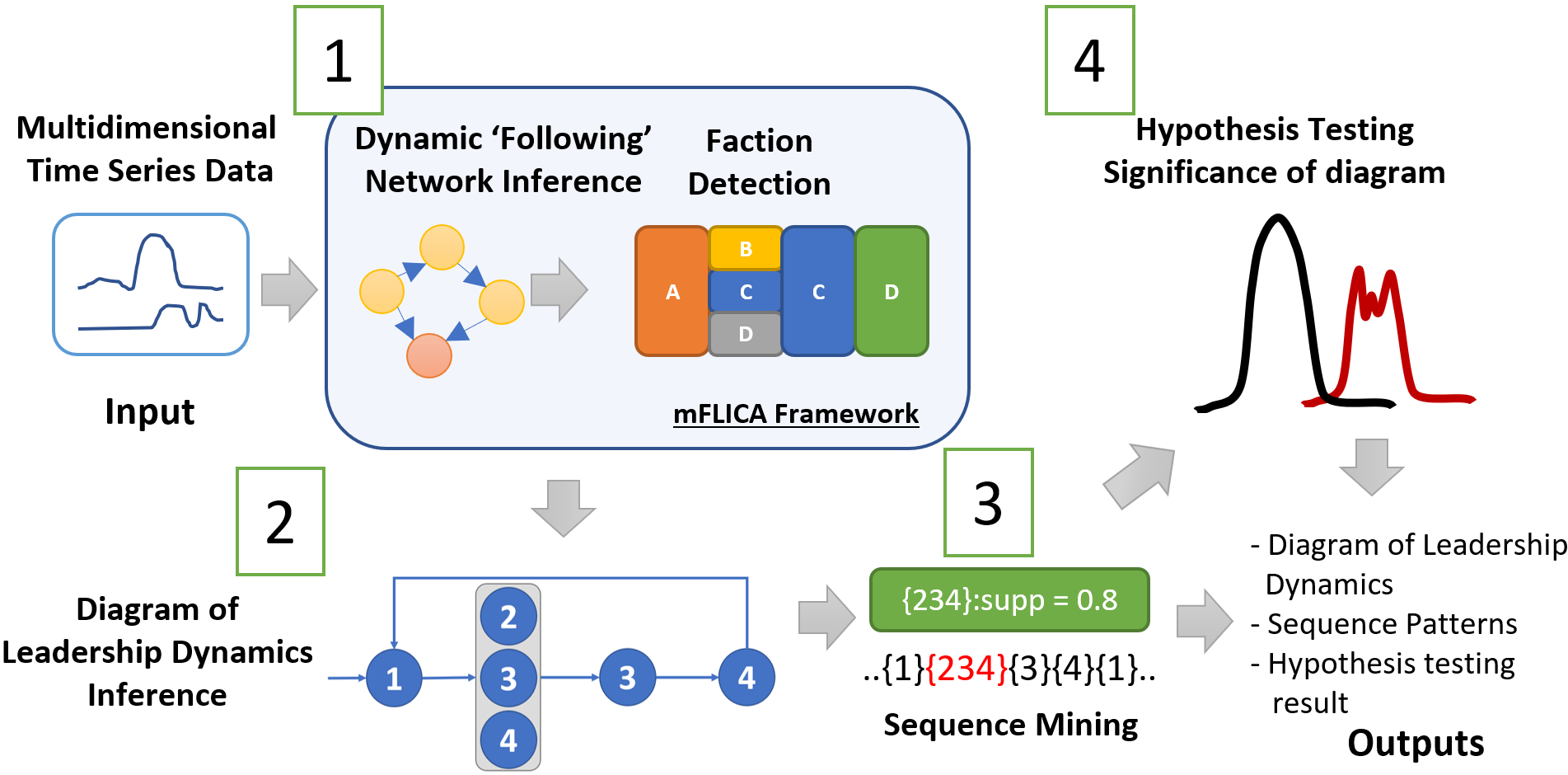
To solve Problem 1, we propose the framework consisting of four parts (Fig. 1). Given a set of time series of movement , where is a two-dimensional time series of length , first, we infer a dynamic following network and time series of leaders using mFLICA framework Amornbunchornvej and Berger-Wolf 2018a (Section 3.2). Second, we infer a diagram of leadership dynamics from in Section 3.3. Third, we detect the sequence patterns on in Section 3.4. Finally, we deploy hypothesis tests to evaluate significance of leadership dynamics compared to our proposed null models in Section 3.5.
3.2 mFLICA
Given a pair of time series and , mFLICA uses Dynamic Time Warping (DTW) Sakoe and Chiba 1978 to infer a following relation. Suppose is an optimal warping path from DTW dynamic programming matrix, where implies matched with in the matrix. Intuitively, if is followed by with the time delay , then . Hence, we can compute the following relation by the equation below.
| (2) |
Suppose we have a similarity threshold , there we say there is a following relation if , where follows if and follows if . We set as a default.
Next, given a time window and a sliding window parameter , we have the time window interval . mFLICA creates a following network for each set of time series within interval of . An edge of a following network is inferred by Eq. 2 with the weight . Hence, after every interval has its following network, we have a dynamic following network of .
Lastly, for each time step , mFLICA uses Breadth First Search (BFS) to infer factions and initiators within a following network . The faction initiators are nodes with out-degree zero and in-degree non-zero. By applying BFS to dynamic following network , we have the time series of leaders as well as the time series of factions as the outputs of this step.
3.3 Inferring transition diagram of leadership dynamics
We use Hidden Markov Model (HMM) Rabiner 1989 to model a diagram of leadership dynamics in Def. 7 and use Baum–Welch algorithm Jelinek et al. 1975 to infer the maximum likelihood estimates of parameters of HMM from the time series of leader . In this setting, we have a set of frequent-leader sets as a set of states in HMM with the support threshold . In HMM, the stochastic transition matrix , which has its size , describes estimated probabilities that a group changes its current set of leaders to another set of leaders (e.g. group merging or splitting.) However, since we are interested only in the events of state changes, we ignore the self-transition probability and normalize to be (Eq. 3), which is the adjacency matrix of .
Given a time series of leaders , we can easily infer a set of leader sets . Then, let be a set of states in HMM where and are in one-to-one correspondence. We represent each state in as a number in , then we create by replacing each element in with the number of corresponding state in . For example, in Fig. 3 (Dynamic Type 1), we have a set of leader sets and , where , and , in have corresponding elements in as and , respectively.
Initially, we set a stochastic transition matrix ( are the states) and the initial state distribution uniformly. We have the set of observation values . In this setting, there is no hidden state since an observation value is an identity of a state. However, in HMM, at any state , there is a required probability of observing value at the state (typically represented by a matrix .) Here, the probability if and zero otherwise.
We use Baum–Welch algorithm Jelinek et al. 1975 to infer , then we normalize to create by the equation below.
| (3) |
3.4 Mining sequence patterns of leadership dynamics
After having a diagram of leadership dynamics , for each pair of nodes , we find a sequence pattern, which is a path , where for all , .
is an order sequence that the previous state has the highest probability to change to the next consecutive state , given a starting point at and the final state at .
Given as an adjacency matrix of , we convert to be where . Then, we use the standard Dijkstra’s algorithm to find the shortest path between every two nodes in . Hence, is the shortest path between and in 11 1 Note, this can be done since the probability condition is independent of each pair and not cumulative over the path. Let be a number of times that the full sequence of occurs in and be a number of times that leadership state change happens in (e.g., two sub-groups merged together, changing the leader), we can find the support of in the time series of leader by the equation below:
| (4) |
Specifically, is a number of times that all pairs of nodes s.t. appear before in also appear in .
3.5 Hypothesis testing
| Method | Null hypothesis |
|---|---|
| Kolmogorov-Smirnov test Massey Jr. 1951 | Two samples are from |
| Wilcoxon Rank Sum Test Wilcoxon 1945 | the same distribution |
| Kruskal-Wallis Test Kruskal and Wallis 1952 |
3.5.1 Evaluating the significance of leadership-event order
Given a time series of leaders and a diagram of leadership dynamics inferred from , we perform a random permutation of elements in to create , then we infer a diagram of leadership dynamics from by the method described by the previous section. Afterwards, we test the similarity of the edge-weight distributions of and . We deploy three non-parametric methods, shown in Table 2, to perform the tests. If all three methods successfully reject the null hypothesis with the significant threshold , then we conclude that the edge-weight distribution of is significantly different from ’s although the support value of each node in both graphs are the same.
3.5.2 Evaluating the significance of frequencies of leadership-event sequences
After finding all the sequences for every pair of nodes in Section 3.4, we compute the support of each sequence . This gives the sequence-support distribution of . Next, we rewire to be by uniformly and randomly changing the end points of each edge in , then we calculate the sequence-support distribution of (Eq. 4.) Lastly, we test whether and sequence-support distributions are different the same way as in the previous section.
We repeat both types of significance tests 100 times and report the percentage of times that the tests successfully reject for each dataset.
3.6 Followership dynamics

Let be a set of time series of movement, where is a time series of length . In the first step, we infer a dynamic following network as well as a time series of factions using mFLICA framework Amornbunchornvej and Berger-Wolf 2018a (Section 3.2).
Second, we infer a co-faction network (Section 3.6.1) and a lead-follow network (Section 3.6.2) from . Afterwards, we infer a set of frequent co-faction clusters (Section 3.6.3).
3.6.1 Co-faction network inference
To infer a co-faction network, the first step is to infer a pair of frequent co-faction in Def. 9.
Given a time series of factions with the length and an indicator function (which is if the statement is true, and otherwise), we define the support of having individuals and in the same faction below.
| (5) |
Here indicates the support of having a particular pair of individuals and being within the same faction in .
After we compute the supports for all pairs of individuals, we have a co-faction network . Given a threshold , there is an edge if . The edge weight of is .
3.6.2 Lead-follow network inference
To infer a lead-follow network, the first step is to infer a frequent leader-follower pair in Def. 11. Given a time series of factions with the length and an indicator function (which is if the statement is true, and otherwise), we can define a support of having individual in the faction lead by an initiator below.
| (6) |
Where is a set of faction members leading by . Here indicates the support of having a particular individual in the faction leading by an initiator in .
After we compute the supports for all pairs of individuals, then we have a lead-follow network . Given a threshold , for any and , there is a directed edge if . The edge weight of is . Higher implies that there is a higher frequency that is a member of ’s faction. Hence, we can use as a proxy of loyalty of to . Higher implies that is more loyal to .
3.6.3 Clustering and cohesion measure
We use the standard Hierarchical clustering with shortest distance to link clusters Sibson 1973 to demonstrate our framework ability. However, any clustering algorithm can be used in our framework to perform the analysis. The Hierarchical clustering algorithm is an agglomerative clustering approach that starts with each individual in a cluster by itself. Then, it keeps merging two closest clusters to be a single new cluster. The algorithm keeps merging on a set of clusters until there is only a single cluster. Given and are clusters and is an adjacency matrix of a co-faction network that has its element as , the distance between two clusters is defined below.
| (7) |
Where represents an th vector row of and is a standard euclidean distance. The reason that we compute the distance between the vector of weights of to all individuals and the vector of weights of to all individuals in is that because two individuals who share the same set of are likely members of the same faction. Hence, they should have a small distance.
Next, since there are two types of edges in : edges that connect members within the same clusters and edges that connect individuals of different clusters. We can use k-means algorithm where to cluster a list of edge weight of the hierarchical tree into two types: internal edges and external edges. Finally, we link any leaves (individuals) of hierarchical tree that are reachable using internal edges to be a member of the same group to represent a frequent co-faction cluster in Def 10.
To measure the degree of cohesion of , we use the standard Modularity Measure (Q value) proposed by M. E. J. Newman and M. Girvan (2004) Newman and Girvan 2004 below.
| (8) |
where is a fraction of edges that have one end connected to a node in a cluster and another end connected to a member of a cluster , and . The value of has a range between and . If the value is a large positive, then there are multiple strong clusters; the numbers of edges within groups are greater than the numbers of edges between groups. When there are multiple subgroups that have higher edge weight within the same cluster while edges that connect nodes from different clusters have lower edge weights, then is close to one. In contrast, if either there is only one cluster or edge weights of all pairs of nodes are not different from each other, then is close to zero. In other words, higher implies higher number of subgroups that have relatively high edge-weight between nodes within the same cluster compared to edge-weights of nodes from different clusters. Hence, we can use as a proxy of cohesion of group. Higher implies lower cohesion.
3.7 Time and space complexity
The time complexity of mFLICA is , where is a number of time series, is a length of time series, and is a time window parameter. The time complexity of BaumWelch algorithm to infer a diagram of leadership dynamics is where is the number of frequent-leader sets. Typically, since there are fewer frequent-leader sets than individuals. In the followership part, we can scan a time series of factions only once to compute everything, which has the time complexity at most . Hence, our framework’s overall time complexity is . For the space complexity, the most expensive part of our framework is the space for the dynamic following network, which is .
3.8 Parameters sensitivity
For the time window parameter , the work by Amornbunchornvej et al. 2018 reported that the following relation is robust to the noise. However, if we set below the maximum time delay between time series, then the result can be severely affected. Hence, a user should try to guess the maximum time delay on his/her dataset before setting . Since the core engine of mFLICA is the following relation measure, it is important to set properly. The other parameter such as significant level should be fine- tuned w.r.t. the task.
4 Evaluation Datasets

We evaluate our method on synthetic datasets generated using a variety of leadership models with a variety of patterns of leadership dynamics.
4.1 Leadership models
There are three leadership models that we consider in this paper below.
4.1.1 Dictatorship Model (DM) Amornbunchornvej and Berger-Wolf 2018a
Initially, all individuals stay in the initial area. Then, a single initiator moves toward a target path before others. Afterwards, all other individuals follow the initiator with some time delay.
4.1.2 Hierarchical Model (HM) Amornbunchornvej and Berger-Wolf 2018a
Each individual has been assigned the unique ranking value at the beginning. Lower rank individuals always follow higher rank individuals. An initiator who has the highest-rank individual (initiator) starts moving first, then the second high-rank individual follows the first-rank individual with sometime delay and so on (the th rank individual follows the th- rank individual).
4.1.3 Independent Cascade Model (IC) Kempe et al. 2003
Initially, all individuals are deactivated. At the beginning, each individual has a chance to be active with the probability . After activation, the active individuals move following the initiator except the initiator itself that follows in the target direction. In every time step, active individuals attempt to activate their -nearest inactive neighbors with the probability of success . Active individuals cannot attempt to activate the same individual twice. In this paper, we determine the parameter space on a combination of : and .
4.2 Synthetic trajectory simulation.
We use simulated datasets to evaluate the performance of our framework. Each dataset consists of 30 individuals. The trajectory of each individual is two-dimensional time series of length 4000 time steps. Each dataset has been generated from one of the three leadership models described above. There are five coordination events in each dataset. One coordination event lasts for 800 time steps. There are two types of coordination events as follows.
4.2.1 Type 1 Dynamics: Splitting/Merging coordination event Amornbunchornvej and Berger-Wolf 2018a
In this type of coordination event (Fig. 3 above), ID1 leads the entire group for 200 time steps. Then, the group splits into three equal size sub-groups lead by ID2, ID3, and ID4, for the duration of 200 time steps. Afterwards, all sub-groups are merged into a single group again lead by ID3 for another 200 time steps. Finally, ID4 leads the entire group for the last 200 time steps.
4.2.2 Type 2 Dynamics: Linear coordination event Amornbunchornvej and Berger-Wolf 2018a
In this type of coordination event (Fig. 3 below), ID1 leads first, then ID2 leads, ID3 leads after ID2, and ID4 leads after ID3. Each leader leads the group for 200 time steps.
After a coordination event ends, then, the group stops moving and the next coordination event repeats the pattern. In this paper, we generated 100 datasets for each leadership model and coordination type (e.g. DM with Type 1 dynamics has 100 datasets). One exception: IC has nine cases of different parameters settings and we have a 100 datasets for each parameter setting and dynamics type. In total, we have 400 datasets for DM and HM but 1800 datasets for IC.
4.3 Baboon Dataset
We also deploy our framework on a dataset of GPS trajectories of wild olive baboons (Papio anubis) living at Mpala Research Centre, Kenya Crofoot et al. 2015; Strandburg-Peshkin et al. 2015. The dataset consists of latitude-longitude location time series of 16 baboons recorded for every second for a nine day period (419,095 time steps). We employ this dataset to demonstrate the potential of our framework to uncover relationships within data to generate scientific hypotheses.
5 Evaluation criteria
5.1 Leadership dynamics
In simulated datasets, we compare the inferred adjacency matrix of a digraph of leadership dynamics against the ground truth matrix . For the Splitting/Merging coordination event, the ground-truth set of frequent-leader sets is
All elements in are zero except
For the Linear coordination event,
and all elements in are zero except
Let and be the predicted and the ground truth sets of frequent-leader sets, respectively. The loss function of and is below:
| (9) |
| (10) |
| (11) |
Where is the number of elements within . The first term in Eq. 9 represents the -norm difference between each element in and (probabilities) when the predicted states are the same as the ground truth. The second term represents the false positive case when the framework predicts the states that do not exist in the ground truth. The last term represents the false negative case when the framework misses prediction of a state that exists in the ground truth.
5.2 Followership dynamics
5.2.1 Co-faction network
In simulated datasets, we compare an inferred adjacency matrix of a co-faction network against the ground truth matrix . All members from the same cluster connected with edges that have the weights
while two nodes from different clusters have the weight
For the Splitting/Merging coordination datasets, the ground-truth is that there are three clusters:
For Linear coordination datasets, all individuals are in the single cluster. Given is a set of nodes of individuals, we use the absolute loss function to evaluate the difference between predicted and the ground truth below:
| (12) |
5.2.2 Lead-follow network
We also compare an inferred adjacency matrix of a lead-follow network against the ground truth matrix of . In both Splitting/Merging and Linear coordination datasets, , and are only initiators. Hence, and .
For Splitting/Merging coordination datasets, given a leader , for any
-
If and , then , while for .
-
If and , then , while for .
-
If and , then , while for .
In Linear coordination datasets, for and ,
Let and be the predicted and the ground truth sets of initiators of a lead-follow network respectively, we compare the inferred and the ground-truth using the loss function below:
| (13) |
Where is the number of elements within .
5.2.3 Clustering evaluation
For Splitting/Merging coordination datasets, the ground truth of first cluster is . The second cluster is . The third cluster is . For linear coordination datasets, all individuals are in the single cluster. We use score to measure the difference between inferred and ground-truth clusters. Given is a ground-truth cluster and is a predicted cluster that have the most common members with . The true positive is a sum of number of common members between all pair of and . The false positive is a sum of number of individuals that are in but not in . and the false negative is a sum of number of individuals that are in but not in .
6 Results
6.1 Leadership dynamics
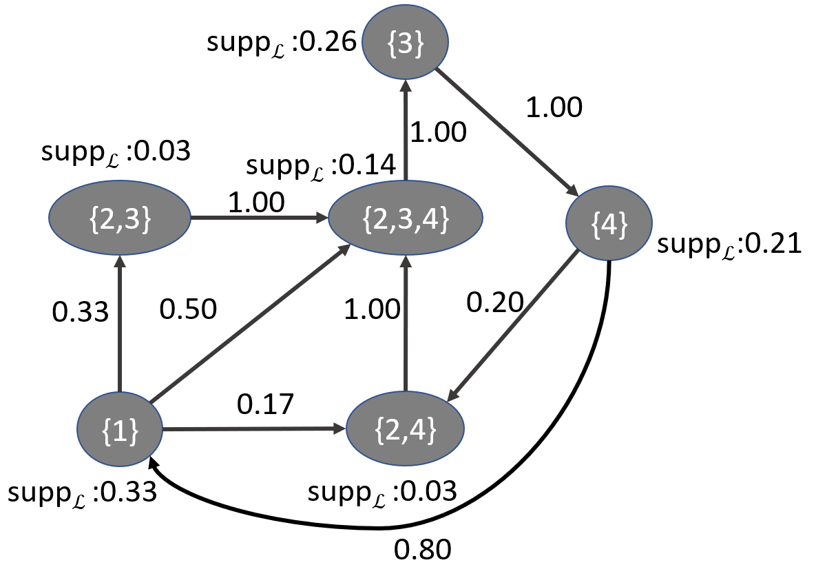
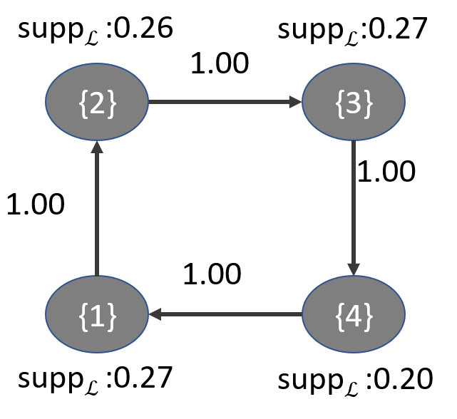
We set the time window parameter using the inference method in Amornbunchornvej and Berger-Wolf 2018a. Fig. 4 and Fig. 5 show the examples of inferred diagrams of leadership dynamics by our framework from Type-1-HM (Hierarchical model with Splitting/Merging coordination events) and Type-2-HM (Hierarchical model with Linear coordination events) datasets respectively. In Fig. 4, comparing the inferred diagram with the ground truth, only nodes and are false positive nodes, both with very low support of 0.03.
This implies that despite the complex dynamics of leadership in Type-1-Dynamics case, our framework was still able to retrieve the diagram of leadership dynamics accurately. For the Type-2-HM dataset, which is less complex than Type1-HM case, Fig. 5 shows that there are no false positive nodes in the inferred diagram. Moreover, in both Type-1-HM and Type-2-HM cases, the support of each node should be , and our framework can infer the support for each node closely to .
Regarding the mining sequence patterns of leadership dynamics described in Section 3.4, Table 3 shows an example of max-support sequences of leadership dynamics that our framework reported from HM datasets. In both dynamics types, the sequences are consistent with the ground truth in Fig. 3.
| Datasets | Sequences | |
|---|---|---|
| Type-1-HM | {2,3,4},{3},{4},{1} | 0.71 |
| Type-2-HM | {1},{2},{3},{4} | 0.95 |
Next, we compared our framework, which uses the following networks concept Amornbunchornvej and Berger-Wolf 2018a, to the method based on direction networks proposed in FLOCK method Andersson et al. 2008 to infer a diagram of leadership dynamics. In direction networks, at any time , if is moving toward the same direction as but is in front of , then follows . The median of all loss distributions in both Type-1 and Type-2 dynamics datasets are reported in Table 4. The first row of Table 4 shows the distribution of loss values (Eq. 9) in Type-1-dynamics datasets. The direction network approach was reasonably competitive for the Type-1 dynamics. We were able to use the direction networks to infer the states with splits and merges but the change of leadership was often missed by this underlying method. Not surprisingly, then, the direction network-based method performed significantly worse than the following network-based approach for the Type-2 dynamics. Qualitatively, and as a distribution of the loss values overall, the following networks as the basis for the diagram inference performed better than the direction networks in our framework. In the second row of Table 4, the following networks also performed better than direction networks in Type-2-dynamics datasets.
| Dyn. Type | Type 1 | Type 2 | ||||
|---|---|---|---|---|---|---|
| Model | HM | DM | IC | HM | DM | IC |
| Following Network | 0.13 | 0.19 | 0.24 | 0 | 0.03 | 0.08 |
| Direction Network | 0.19 | 0.19 | 0.25 | 0.19 | 0.19 | 0.25 |
In Table 5, we reported the hypothesis testing results of the significance of leadership-event order (Section 3.5.1). With respect to the type of the leadership model, for the HM, which is a well-structure model, the inferred diagrams are more significantly different from the null-model diagram than for the other leadership models. With respect to the types of the dynamics, in the complex type-1-dynamics datasets our framework inferred diagrams that are more significantly different from the null model. Lastly, the following networks were able to infer diagrams that are more different from the null model than the direction networks.
| Dyn. Type | Type 1 | Type 2 | ||||
|---|---|---|---|---|---|---|
| Model | HM | DM | IC | HM | DM | IC |
| Following Network | 0.99 | 0.55 | 0.38 | 0.86 | 0.08 | 0.20 |
| Direction Network | 0.00 | 0.00 | 0.06 | 0.00 | 0.00 | 0.06 |
For hypothesis testing of the significance of frequencies of leadership-event sequences (Section 3.5.2), the result is shown in Table 6. Similar to the the edge-weight distribution testing, the support distributions of the well-structure model, HM, are significantly different from the support distribution of the null model. The following networks also can be used to infer diagrams that are different from the rewiring diagrams than the direction networks based approach. However, in the simple type-2-dynamics datasets, our framework was able to infer diagrams that are more different from the null model compared to the complex type-1-dynamics case.
| Dyn. Type | Type 1 | Type 2 | ||||
|---|---|---|---|---|---|---|
| Model | HM | DM | IC | HM | DM | IC |
| Following Network | 0.95 | 0.35 | 0.23 | 0.94 | 0.84 | 0.66 |
| Direction Network | 0.07 | 0.08 | 0.20 | 0.07 | 0.07 | 0.20 |
For the baboon dataset, we reported the information that we can retrieve from the dataset using our framework as a case study. Fig. 6 shows the inferred diagram of leadership dynamics from our framework. Each row represents the node of leader sets of previous state and each column represents the next state. Each row label consists of baboon gender: ‘M’ or ‘F’, a set of frequent-leader IDs, and the support value of frequent-leader set. For example, in row 3 and column 2, the event that two female baboons F18 and F22 are leading their separate sub-groups concurrently can happen with the support 0.1 (out of all the coordination times). These two sub-groups have a chance to be merged together to a larger group lead by F18 with the probability 0.29. In 4th column (F9), we found that no matter what the previous sub-groups were, there was a high chance that the next group would be lead solely by the female baboon F9. In 4th row, F9 has the highest support (0.19), which means F9 (who happens to be the dominant female) often leads the troop, with the next highest support of 0.11 for the male baboon M3 (5th column, the alpha male). Lastly, at row 5 and column 4, if M3 and F9 are leading their separate sub-groups, then the two groups will be merged to a larger group lead by F9 with probability 0.63.
The hypothesis testing of the edge-weight distribution shows that the baboon’s diagram is significantly different from the null model, with 100% of the time the tests successfully rejecting . However, for the hypothesis testing of sequence-support distributions, the baboons’ sequences of leadership dynamics are not significantly different from the rewired diagram. Only 5% of the times the tests successfully reject . This indicates that while individual leaders identity is non-random and pairwise leadership transition patterns are significant, there are no leadership sequences that often appear significantly within the baboon dataset. Nevertheless, Table 7 shows baboons’ sequences of leadership dynamics that have the top-4 highest support. This result is the evidence that F9 is an important individual who frequently leads the group.
| Baboon | Sequences | |
|---|---|---|
| Seq. 1 | {M11},{F9},{M3} | 0.0354 |
| Seq. 2 | {M18},{F9},{M3} | 0.0354 |
| Seq. 3 | {M18},{F9},{M22} | 0.0354 |
| Seq. 4 | {M4},{F9},{M2} | 0.0354 |
These results show that our framework provides the opportunity for scientists to gain more insight into their datasets in order to generate scientific hypotheses, which might lead to important scientific discoveries (in this case, about the collective behavior and leadership dynamics of social animals).

6.2 Followership dynamics
6.2.1 Co-faction and lead-follow networks

Fig. 7 shows the results of ground-truth and predicted adjacency matrices of co-faction network by our framework from Type-1-HM (Hierarchical model with Splitting/Merging coordination events) and Type-2-HM (Hierarchical model with Linear coordination events) datasets. Each predicted matrix is the result of aggregation of co-faction adjacency matrices from 100 datasets. The result shows that our inferred matrices are mostly similar to the ground-truth matrices with some variation due to noise. ID4 has the highest error in Fig. 7 since it appears during the interval when the group stop moving. Because mFLICA is designed to handle movement initiation analysis, it has a limitation to analyze stopping intervals of movement. Hence, mFLICA cannot capture the behavior of a leader ID4 well.
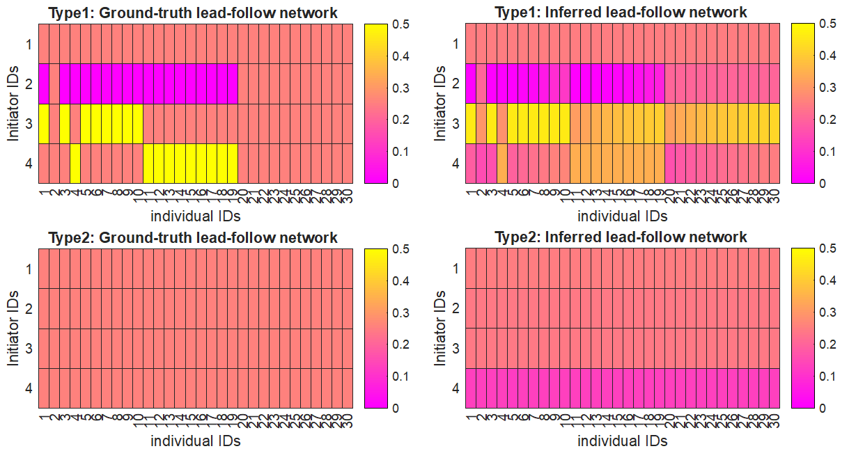
Fig. 8 shows the results of ground-truth and predicted adjacency matrices of lead-follow networks with . Each predicted matrix is the result of aggregation of lead-follow adjacency matrices from 100 datasets. The result also shows that our inferred matrices are mostly similar to the ground-truth matrices with some variation. ID4 result has the highest error because of mFLICA limitation that we have just discussed.
| Following Network | Direction Network | |||
|---|---|---|---|---|
| Type-1 | Type-2 | Type-1 | Type-2 | |
| Co-fact loss | ||||
| Lead-foll loss | ||||
We also report the quantitative result of prediction of both co-faction and lead-follow networks using following networks compared with direction networks in Table 8. Overall, our proposed framework using following networks performed better than the direction network framework. For co-faction networks, the loss values are higher than lead-follow network loss values. This implies that finding who are in the same faction frequently is a bit harder than finding who are loyal members of specific leaders.
6.2.2 Clustering results
| Our framework | NM community detection | |
|---|---|---|
| Type-1 dynamics | ||
| Type-2 dynamics |
In the clustering task, given a co-faction network as an input, we compared our proposed framework with a standard community detection algorithm in Newman 2004. The NM community detection method greedily searches for the partition of individuals that maximize the Q-value in Eq. 8. Table 9 shows the result of Q-values of our framework and NM community detection. For type-1 dynamics, we should have a high value of -value since there are three strong clusters. Table 9 shows that even though NM method tried to find the best clustering partition that maximizes Q-value, our framework found a set of better clusters that has a higher Q-value than NM’s clusters. For type-2 dynamics, since there is only one cluster, we expect that the Q-value should be close to zero. Both methods performed well in this case.
| Our framework | NM clustering | |
|---|---|---|
| Type-1 dynamics | ||
| Type-2 dynamics |
We also reported the results of clustering comparison between the ground-truth and inferred clusters. The result in Table 10 shows that our framework performed better than NM in both types of dynamics.
6.3 Baboon followership dynamics
For the baboon dataset, we reported the result of co-faction clustering (Fig. 9) and lead-follow network (Fig. 10) inferred from the trajectories of baboon during pre-coordination intervals of high-coordination events.

Fig. 9 shows five major clusters in the dataset. The interesting cluster is the cluster of ID3 and ID9. ID3 is an alpha male while ID9 is an alpha female. Since they are in the same cluster, this implies that they might be a couple.

7 Conclusion
In this paper, we proposed a new approach to analyze time series of group movement data. We formalized a new computational problem, Mining Patterns of Leadership Dynamics, and Mining Patterns of Followership Dynamics, as well as proposed a framework as a solution of these problems. Our framework can be used to address several questions regarding leadership and followership dynamics of group movement, such as ‘what is the probability of having two sub-groups lead by and being merged together to be a larger group lead by later?’, ‘what is the frequency of having and co-leading their sub-groups concurrently?’, ‘how likely is it that a specific sub-group that is a member will be leading by an individual from the same faction?’, etc. We use the leadership inference framework, mFLICA Amornbunchornvej and Berger-Wolf 2018a, to infer the time series of leaders and their factions from movement datasets, then propose an approach to mine and model frequent patterns of both leadership and followership dynamics. We evaluate our framework performance by using several simulated datasets, as well as the real-world dataset of baboon movement to demonstrate the applications of our framework. These are novel computational problems and, to the best of our knowledge, there are no existing comparable methods to address them. Thus, we modify and extend an existing leadership inference framework to provide a non-trivial baseline for comparison. Our framework performs better than this baseline in all datasets. Our framework opens the opportunities for scientists to generate testable scientific hypotheses about the dynamics of leadership in movement data.
References
- Aggarwal and Han (2014) Aggarwal CC, Han J (2014) Frequent pattern mining. Springer
- Agrawal et al. (1993) Agrawal R, Imieliński T, Swami A (1993) Mining association rules between sets of items in large databases. In: Proceedings of the 1993 ACM SIGMOD International Conference on Management of Data, ACM, New York, NY, USA, SIGMOD ’93, pp 207–216, DOI 10.1145/170035.170072, URL http://doi.acm.org/10.1145/170035.170072
- Amornbunchornvej and Berger-Wolf (2018a) Amornbunchornvej C, Berger-Wolf T (2018a) Framework for inferring leadership dynamics of complex movement from time series. In: Proceedings of the 2018 SIAM International Conference on Data Mining, SIAM, pp 549–557, DOI 10.1137/1.9781611975321.62, URL https://epubs.siam.org/doi/abs/10.1137/1.9781611975321.62, https://epubs.siam.org/doi/pdf/10.1137/1.9781611975321.62
- Amornbunchornvej and Berger-Wolf (2018b) Amornbunchornvej C, Berger-Wolf TY (2018b) Mining and modeling complex leadership dynamics of movement data. In: ASONAM’18, IEEE, pp 447–454, DOI 10.1109/ASONAM.2018.8508310
- Amornbunchornvej et al. (2018) Amornbunchornvej C, Brugere I, Strandburg-Peshkin A, Farine DR, Crofoot MC, Berger-Wolf TY (2018) Coordination event detection and initiator identification in time series data. ACM Trans Knowl Discov Data 12(5):53:1–53:33, DOI 10.1145/3201406, URL http://doi.acm.org/10.1145/3201406
- Andersson et al. (2008) Andersson M, Gudmundsson J, Laube P, Wolle T (2008) Reporting leaders and followers among trajectories of moving point objects. GeoInformatica 12(4):497–528
- Couzin et al. (2005) Couzin ID, Krause J, Franks NR, Levin SA (2005) Effective leadership and decision-making in animal groups on the move. Nature 433(7025):513–516
- Crofoot et al. (2015) Crofoot MC, Kays RW, Wikelski M (2015) Data from: Shared decision-making drives collective movement in wild baboons
- Glowacki and von Rueden (2015) Glowacki L, von Rueden C (2015) Leadership solves collective action problems in small-scale societies. Phil Trans R Soc B 370(1683):20150010
- Han et al. (2007) Han J, Cheng H, Xin D, Yan X (2007) Frequent pattern mining: current status and future directions. Data Mining and Knowledge Discovery 15(1):55–86, DOI 10.1007/s10618-006-0059-1, URL https://doi.org/10.1007/s10618-006-0059-1
- Hogg (2001) Hogg MA (2001) A social identity theory of leadership. Personality and social psychology review 5(3):184–200
- Jelinek et al. (1975) Jelinek F, Bahl L, Mercer R (1975) Design of a linguistic statistical decoder for the recognition of continuous speech. IEEE Transactions on Information Theory 21(3):250–256
- Kempe et al. (2003) Kempe D, Kleinberg J, Tardos É (2003) Maximizing the spread of influence through a social network. In: Proceedings of the ninth ACM SIGKDD, ACM, pp 137–146
- Keogh and Ratanamahatana (2005) Keogh E, Ratanamahatana CA (2005) Exact indexing of dynamic time warping. Knowledge and information systems 7(3):358–386
- Kjargaard et al. (2013) Kjargaard MB, Blunck H, Wustenberg M, Gronbask K, Wirz M, Roggen D, Troster G (2013) Time-lag method for detecting following and leadership behavior of pedestrians from mobile sensing data. In: Proceedings of the IEEE PerCom, IEEE, pp 56–64
- Krause et al. (2000) Krause J, Hoare D, Krause S, Hemelrijk C, Rubenstein D (2000) Leadership in fish shoals. Fish and Fisheries 1(1):82–89
- Kruskal and Wallis (1952) Kruskal WH, Wallis WA (1952) Use of ranks in one-criterion variance analysis. Journal of the American Statistical Association 47(260):583–621, DOI 10.1080/01621459.1952.10483441, URL https://www.tandfonline.com/doi/abs/10.1080/01621459.1952.10483441, https://www.tandfonline.com/doi/pdf/10.1080/01621459.1952.10483441
- Lee et al. (2007) Lee JG, Han J, Whang KY (2007) Trajectory clustering: a partition-and-group framework. In: Proceedings of the 2007 ACM SIGMOD international conference on Management of data, ACM, pp 593–604
- Li et al. (2010) Li Z, Lee JG, Li X, Han J (2010) Incremental clustering for trajectories. In: Kitagawa H, Ishikawa Y, Li Q, Watanabe C (eds) Database Systems for Advanced Applications, Springer Berlin Heidelberg, Berlin, Heidelberg, pp 32–46
- Massey Jr. (1951) Massey Jr FJ (1951) The kolmogorov-smirnov test for goodness of fit. Journal of the American Statistical Association 46(253):68–78, DOI 10.1080/01621459.1951.10500769, URL https://amstat.tandfonline.com/doi/abs/10.1080/01621459.1951.10500769, https://amstat.tandfonline.com/doi/pdf/10.1080/01621459.1951.10500769
- Newman (2004) Newman MEJ (2004) Fast algorithm for detecting community structure in networks. Phys Rev E 69:066133, DOI 10.1103/PhysRevE.69.066133, URL https://link.aps.org/doi/10.1103/PhysRevE.69.066133
- Newman and Girvan (2004) Newman MEJ, Girvan M (2004) Finding and evaluating community structure in networks. Phys Rev E 69:026113, DOI 10.1103/PhysRevE.69.026113, URL https://link.aps.org/doi/10.1103/PhysRevE.69.026113
- Rabiner (1989) Rabiner LR (1989) A tutorial on hidden markov models and selected applications in speech recognition. Proceedings of the IEEE 77(2):257–286, DOI 10.1109/5.18626
- Sakoe and Chiba (1978) Sakoe H, Chiba S (1978) Dynamic programming algorithm optimization for spoken word recognition. IEEE transactions on acoustics, speech, and signal processing 26(1):43–49
- Shokoohi-Yekta et al. (2015) Shokoohi-Yekta M, Wang J, Keogh E (2015) On the non-trivial generalization of dynamic time warping to the multi-dimensional case. In: SDM’15, pp 289–297
- Sibson (1973) Sibson R (1973) Slink: An optimally efficient algorithm for the single-link cluster method. The Computer Journal 16(1):30–34, DOI 10.1093/comjnl/16.1.30, URL http://dx.doi.org/10.1093/comjnl/16.1.30, /oup/backfile/content_public/journal/comjnl/16/1/10.1093/comjnl/16.1.30/2/160030.pdf
- Smith et al. (2015) Smith JE, Estrada JR, Richards HR, Dawes SE, Mitsos K, Holekamp KE (2015) Collective movements, leadership and consensus costs at reunions in spotted hyaenas. Animal Behaviour 105:187–200
- Spiliopoulou et al. (2006) Spiliopoulou M, Ntoutsi I, Theodoridis Y, Schult R (2006) Monic: Modeling and monitoring cluster transitions. In: Proceedings of the 12th ACM SIGKDD International Conference on Knowledge Discovery and Data Mining, ACM, New York, NY, USA, KDD ’06, pp 706–711, DOI 10.1145/1150402.1150491, URL http://doi.acm.org/10.1145/1150402.1150491
- Strandburg-Peshkin et al. (2015) Strandburg-Peshkin A, Farine DR, Couzin ID, Crofoot MC (2015) Shared decision-making drives collective movement in wild baboons. Science 348(6241):1358–1361, DOI 10.1126/science.aaa5099, URL http://science.sciencemag.org/content/348/6241/1358, http://science.sciencemag.org/content/348/6241/1358.full.pdf
- Stueckle and Zinner (2008) Stueckle S, Zinner D (2008) To follow or not to follow: decision making and leadership during the morning departure in chacma baboons. Animal Behaviour 75(6):1995–2004
- Tantipathananandh et al. (2007) Tantipathananandh C, Berger-Wolf T, Kempe D (2007) A framework for community identification in dynamic social networks. In: Proceedings of the 13th ACM SIGKDD International Conference on Knowledge Discovery and Data Mining, ACM, New York, NY, USA, KDD ’07, pp 717–726, DOI 10.1145/1281192.1281269, URL http://doi.acm.org/10.1145/1281192.1281269
- Wilcoxon (1945) Wilcoxon F (1945) Individual comparisons by ranking methods. Biometrics Bulletin 1(6):80–83, URL http://www.jstor.org/stable/3001968