Affine Linear Parameter-Varying Embedding of Nonlinear Models with Improved Accuracy and Minimal Overbounding
Abstract
In this paper, automated generation of linear parameter-varying (LPV) state-space models to embed the dynamical behavior of nonlinear systems is considered, focusing on the trade-off between scheduling complexity and model accuracy and on the minimization of the conservativeness of the resulting embedding. The LPV state-space model is synthesized with affine scheduling dependency, while the scheduling variables themselves are nonlinear functions of the state and input variables of the original system. The method allows to generate complete or approximative embedding of the nonlinear system model and also it can be used to minimize complexity of existing LPV embeddings. The capabilities of the method are demonstrated on simulation examples and also in an empirical case study where the first-principle motion model of a 3-DOF control moment gyroscope is converted by the proposed method to LPV model with low scheduling complexity. Using the resulting model, a gain-scheduled controller is designed and applied on the gyroscope, demonstrating the efficiency of the developed approach.
1 Introduction
The linear parameter-varying (LPV) framework has been introduced to tackle the control problem of nonlinear (NL) and time-varying (TV) systems using the extension of powerful linear control methods Rugh and Shamma 2000b. This methodology offers great potential in a wide variety of practical applications Hoffmann and Werner 2015. By using so-called scheduling variables, which express nonlinear or time-varying behavior, LPV systems are capable of representing the solution set of NL/TV systems in terms of a linear structure. Extension of linear-time invariant (LTI) methods to exploit this linear proxy representation has seen a tremendous development Hoffmann and Werner 2015; however, the lack of systematic methods that are capable of automatically deriving LPV embeddings of NL/TV systems has prevented the widespread industrial use of the LPV concept Toth 2010.
While LPV system identification methods have matured over the last 15 years with many competitive approaches, e.g. Tóth et al. 2012; Goos and Pintelon 2016; Laurain et al. 2012; Tóth et al. 2012; Zhao et al. 2012; Bachnas et al. 2014; Toth 2010; Liu et al. 2019 to mention a few, conversion methods of existing NL/TV models of applications has seen only moderate progress. As in practice, often high-fidelity models of the target application are available due to the development and design process, e.g. rigid body/flexible motion dynamics in mechatronic applications. The need for embedding approaches in which such models are converted to LPV description to be used for control design or prediction purposes is of great significance.
Existing methods can be categorized as local and global methods. In local LPV model conversion, an NL description of the system is linearized at several operating points, then the obtained linearized models are interpolated to get an LPV model. However, due to the local information on the dynamic aspects, closed-loop stability and performance cannot be guaranteed by controllers, designed based on the resulting LPV models, unless the variation of the scheduling variable is guaranteed to be sufficiently slow, see Toth 2010; Bachnas et al. 2014 for an overview. In global methods, the NL/TV system model is directly converted to an LPV representation such that the original system behavior is embedded in the solution set of the resulting LPV model. The methods can be categorized as substation-based transformation methods and (automated) model transformation methods. In substitution based transformation techniques, NL terms are considered to be absorbed by the introduced scheduling variables, which results in a global LPV embedding of NL dynamics; nevertheless, the applicability of these approaches is either limited to a narrow class of NL systems (e.g., Shin et al. 2002; Marcos and Balas 2004) or the methods are based on commonly used, but ad-hoc substitutions (e.g., Zin et al. 2006; Rugh and Shamma 2000a). In the so-called velocity linearization Leith and Leithhead 1998, differentiating the NL state-space model of a system, a representation in terms of derivatives of the inputs, outputs, and state variables multiplied by some nonlinear functions are obtained. Considering these nonlinearities as the scheduling, an LPV model is developed, but requiring specialized control synthesis methods. Model transformation methods are based on the systematic exploration of possible ways of reformulating the NL system as an LPV model with the smallest possible conservatism. Next to the computationally intensive methods in Toth 2010, recent developments include approaches based on linear fractional representation (LFR) with a nonlinear feedback block converted to an LPV model depending affinly on the scheduling variables in Schoukens and Toth 2018. Choosing a LPV embedding for nonlinear systems is investigated in Robles et al. 2019 by minimizing the projection of the nonlinearities onto directions deleterious for performance. The later problem is cast as a computationally intensive linear matrix inequality (LMI) based optimization. A systematic embedding method to achieve a state-minimal LPV representation in the observable canonical form is presented in Abbas et al. 2014. Besides the problem of LPV embedding, reduction of complexity in sense of reducing the number of scheduling variables, simplification of the dependency on the scheduling variables, and tightening the admissible region of the scheduling variables have received attention in recent years. In Kwiatkowski and Werner 2008, taking advantage of principal component analysis (PCA) applied on the typical scheduling trajectories, a method is proposed to obtain LPV models with fewer scheduling variables. It is alleged that the procedure can lead to less overbounding of admissible regions for the scheduling variables without providing a rigorous proof. As an extension to that method, a linear fractional transformation (LFT)-based LPV representation for descriptor systems is proposed in Hoffmann and Werner 2015. The drawback related to these approaches is that they mainly focus on the scheduling variables not their effects on the dynamical behavior of the system. An approach based on Ho-Kalman algorithm is presented in Siraj et al. 2012 to address the problem of joint state-order and scheduling-dependency reduction but applicability of this approach is limited to small scale problems.
In summary, next to accurate representation of the behavior of the NL/TV system, the three main challenges that LPV embedding methods need to face with are (i) scheduling complexity minimization, (ii) minimization of conservativeness of the embedding, (iii) preservation of structural properties like controllability, stability, etc. Most LPV controller synthesis methods rely on linear or quadratic optimization with LMI constraints Scherer 2001; Hjartarson et al. 2015; Caigny et al. 2008; Daafouz et al. 2008; Sato and Peaucelle 2013; Sadeghzadeh 2019; Hanema et al. 2019, the number of which grows exponentially with the scheduling dimension/number of vertices used to describe the scheduling range. Therefore, in terms of problem (i), achieving a minimum number of scheduling variables in LPV modeling has paramount importance in practice. Moreover, many methods are formulated for LPV state-space representations with affine dependence on the scheduling variables, while for mechatronic and chemical systems, straightforward manual conversion results in rational or even exponential dependence that is often hidden in new scheduling variables, leading to at least doubling of the scheduling dimension. Regarding problem (ii), the scheduling variables are usually assumed to vary independently in some specified ranges; while as the above discussion exemplify it, they are functions of some measurable variables of the system with often complicated nonlinear dependence. Thus, the scheduling variable dependency in practice leads to conservativeness of LPV models due to the fact that represented solutions include the solution set of the embedded nonlinear system plus those trajectories that result due to forgetting the above mentioned dependence. This is the price to be paid for a linear representation of the dynamics, but excessive conservativeness can lead to degradation of the achievable performance or even feasibility by LPV control as all extra dynamics resulting purely from conversion are needed to be stabilized and shaped during control synthesis. To the best of our knowledge, a general approach for LPV embedding of nonlinear systems in which the aforementioned factors (i)-(iii) are all appropriately addressed is not available yet. This paper aims to address problems (i)-(ii) and balance complexity, conservativeness and accuracy in LPV model conversion in terms of a practically applicable method.
Three typical problem settings connected to model conversion are considered, namely (a) embedding of nonlinear systems to obtain LPV state-space representation with affine dependence on the scheduling variables and minimal conservativeness; (b) simplifying the dependency of an LPV model depending nonlinearly on the scheduling variables to an affine LPV state-space representation with minimal conservativeness; (c) constructing an affine LPV model with restricted number of scheduling variables from an affine LPV model having too many scheduling variables. Our first contribution is to show that these problem formulations can be uniformly expressed as a single realization problem. Then, by deriving an extension of the approach in Kwiatkowski and Werner 2008, we apply principle component analysis (PCA) to solve the minimal scheduling variable realization problem under affine dependency of the resulting LPV state-space form using a bundle of generated state and input trajectories of the system along which the variation of state-equations are expressed. Contrary to the method of Kwiatkowski and Werner 2008 in which the PCA is applied on the data matrix consisting of the individual scheduling variable trajectories, our contribution is to consider variation of the state-equations directly which, as shown through examples, leads to further reduction of the scheduling complexity. Additionally, an accuracy index is defined to address the trade-off between the number of scheduling variables and the model accuracy, which facilitates determining the number of scheduling variables that are required for the embedding. To minimize conservativeness, we optimize the scheduling range in terms of a minimal hyper-rectangle. Our contribution is to formulate this scheduling range minimization problem and the connected rotational problem of the scheduling space. To reveal the advantages of the proposed method over the existing approaches, the presented method in this paper is applied on simulation examples and validated empirically on a 3-DOF gyroscope system. In the later case, using the obtained LPV model, a full-order gain-scheduled output feedback controller is designed on the converted low complexity model and verified on the experimental setup.
Notation: denotes the elements of matrix , i.e. . refers to row-wise vectorization of :
For , the reverse operation is
The notation corresponds to the Frobenius norm. For a vector function , denotes the empirical standard deviation of the elements of over a data set :
where
with A function is called class if it is continuous and its first derivative exits.
2 Problem statement
Consider an NL system defined by the finite dimensional state-space (SS) representation:
| (1a) | ||||
| (1b) | ||||
where is the state variable, is the input , and is the output of the system for which it is true that satisfies (1) in the ordinary sense. and are considered to be open sets containing the origin.
Assumption 1
It is assumed that the nonlinear functions and are factorisable as
| (2a) | ||||
| (2b) | ||||
where , , , and are bounded and smooth functions on . This is a mildly restrictive assumption, as a wide class of nonlinear systems can be represented by (2), such as rational or polynomial nonlinear systems.
It is supposed that for all initial condition at any , there exists a unique solution which is forward complete. Based on these assumptions, denote the solution set, i.e. the so-called behavior, of the system represented by (1) as
| (3) |
Introduce the notation . Factorization (2) implies the following SS representation for (1):
| (4a) | ||||
| (4b) | ||||
In this paper, three types of problems are tackled.
Problem 1 (Embedding a nonlinear model into an affine LPV model): Find an LPV-SS representation for (4) in the form of
| (5a) | ||||
| (5b) | ||||
such that is a bounded smooth vector function, is a convex set, and matrix functions , , , and have affine dependence on , i.e.,
| (6) |
where represents any of the matrix functions . Let us define the solution set of (5) as follows:
| (7) |
Note that , due to the fact that can get any value in the admissible set irrespective of the values of and . For this problem, the goal is to minimize in terms of a measure on among all possible choices of , , and .
Additionally, one can alternatively seek an approximate affine LPV model as follows:
| (8a) | ||||
| (8b) | ||||
where and by minimizing a measure of discrepancy between the matrices and , which measure is precisely defined later in this section.
Problem 2 (Converting an LPV model with nonlinear dependency on the scheduling variables into an affine LPV model): Given an LPV embedding of (1) in the form of
| (9a) | ||||
| (9b) | ||||
for which , , , and are non-affine functions of the scheduling variable with . In practice, such an embedding can easily happen in case of manual conversion of an NL model to an LPV form (e.g. in case of mechatronic systems (see Sec. 7), direct substitution of the position dependency in the inertia matrices with scheduling variables leads to LPV-SS representations with rational dependence). The goal is to find , , and in terms of (5) and (6) such that the discrepancy between the matrices and is minimized. As in our setting LPV models represent an underlying NL system, we will consider this minimization over all realizations of and in terms of and .
Problem 3 (Obtaining an affine LPV model with reduced number of scheduling variables from an affine LPV model): Given an LPV embedding of (1) in terms of (9), where the state-space matrices are affine functions of . The goal is to find an approximate LPV model (8) such that the discrepancy between the matrices and is minimized over all realizations of and in terms of and . This problem represents the case when the initial number of scheduling variables and/or the admissible set for are non-minimal or further reduction of these is required for feasibility of control synthesis.
Indeed, the mentioned problems are all low complexity embedding problems for either nonlinear or complex LPV systems. The objective is to find an LPV model, affine with respect to a set of constructed scheduling variables, while the accuracy and the conservativeness of the resulting embedding is taken into account. Next we show that Problems 1-3 can be considered under a unified setting. Introduce the representation
| (10) |
where
with , The variables are assumed to lie in a hyper-rectangle , which is the Cartesian product of intervals
where and are a priori known. Thus, . Then Problems 1-3 are represented as follows:
- •
Problem 1: is a NL matrix function of and is defined as follows:
(11) - •
Problem 2: is a NL matrix function of the scheduling variable and defined as follows:
(12) - •
Problem 3: is an affine function of scheduling variable and is defined as in (12).
Let us define
where . The ultimate goal in this paper is to find an LPV model with affine dependency
| (13) |
for (10) by introducing an affine mapping
| (15) |
such that an accuracy index (defined next) is minimized for a prescribed value of . Alternatively, the number of scheduling variables can be chosen by the designer based on the accuracy index value obtained for different number of scheduling variables. The hyper-rectangle set denoted by
| (16) |
is characterized by its lower and upper bounds and . The mapping should be determined in such a way that the volume of is kept at its possible minimum to minimize the conservativeness of the obtained model.
Under the assumption that a data set, representative w.r.t. typical operation of the system (10) (bundle of measured trajectories, equidistant griding of , etc.) is available, we chose the accuracy index as the weighted norm:
| (17) |
where
with , sampling time and weighting
| (19) |
Note that the Frobenius norm of a matrix is a convenient metric to quantify the approximation error of matrices based on singular value decomposition (SVD) type of projections and makes it possible to give explicit characterization of their approximation error. As it becomes clear later, our proposed method is based on such an SVD type of approximation, hence, the Frobenius norm is a natural choice of performance measure for our method. However, it is just a particular choice of norm and other matrix norms can be utilized for this purpose, although other choices lose the connection with the SVD based projection. In the subsequent sections, the problem of finding the mapping , introduced in (2), is addressed.
3 Parameter set mapping
To compute the scheduling mapping, PCA is applied on the data matrix (18), inspired by the method in Kwiatkowski and Werner 2008. Note that contrary to the method in Kwiatkowski and Werner 2008, PCA is applied on the data matrix , capturing the time-domain trajectories of all the elements of the state-space matrices, not only the scheduling trajectories. As we will show, this not only allows to jointly treat Problems 1-3, but it also allows achieving more accurate models with less number of scheduling variables compared to Kwiatkowski and Werner 2008.
First, let us define the affine projection law as follows:
| (20) |
where and are respectively the standard deviation and the mean of over the data set . Now, we can define which means that the corresponding affine mappings are applied on the related elements of the vector . Similarly, we can introduce and the overall to obtain a scaled (unit variance), zero mean representation of the variation of the state-space matrices. Let
| (21) |
be the SVD of . Singular values indicate the principal components of the data. Small singular values indicate relatively unimportant components Olver and Shakiban 2006, which means that projection onto a low-dimensional subspace spanned by the dominant singular vectors will not cause losing too much information. Suppose that are considered as the significant singular values (based on their relative magnitudes). By neglecting the singular values and partitioning , , and V as follows:
where and , one can obtain the following approximation for
| (22) |
where denotes the rescaling and translation, respectively, such that .
Let us define the affine reduced mapping
| (23) |
considering (18) and (22), one can see that
where
| (24) |
Subsequently, one can define
| (25) |
Note that is an affine function of , and is also an affine function of . Thus, is an affine function of , but depending on the function (original dependencies of the state-matrices) can be a nonlinear function of . Based on a well-known matrix approximation lemma Eckart and Young 1936, we have
| (26) |
Bear in mind that is an affine transformation. Therefore, one can easily see that where the matrix is given by (19). This immediately implies
| (27) |
Note that belongs to a hyper-rectangle denoted by
The lower and upper bounds and are obtained respectively as the minimum and maximum values of in terms of (23) over all admissible values of .
Taking into account that depends affinely on the newly introduced scheduling vector , which is in turn an affine vector function of the elements of , one can see that the embedding Problems 1-3 have been successfully addressed. In the next section, the reduction of the associated conservativeness with the LPV models is investigated.
Remark 1
Note that the number of elements of in Problem 1 is usually greater than the number of individual nonlinear functions that appear in . In this case, some of the singular values become zero. If is chosen equal to the number of nonzero singular values, then an exact LPV model is obtained (see 6.2), and an approximate LPV model is obtained if is selected smaller than the number of nonzero singular values. However, for Problems 2 and 3, usually an approximate affine LPV model is developed where the approximation error is characterized by the accuracy index (17).
4 Minimal enclosing hyper rectangles
The hyper rectangle set contains the new scheduling variable ; however, is not necessarily the hyper rectangle with the smallest volume. In this section, we would like to introduce an invertible affine transformation consisting of translation and rotation as follows:
such that the hyper rectangle , denoted by (16), has the minimum possible volume. The problem to find the hyper rectangle with the minimum possible volume can be cast as the problem of finding a hyper rectangle with minimum-volume enclosing a set of points. We consider two distinct cases and for reasons that will be clear soon.
4.1 The case when
Finding the minimum volume enclosing hyper rectangle has already been tackled for two- and three-dimensional point sets in the literature Freeman and Shapira 1975; Toussaint 1983; O’Rourke 1985. In Barequet and Har-Peled 2001, finding a minimum-volume bounding box for a set of points in is considered where an efficient -time algorithm for computing a -approximation of the minimum-volume bounding box is solved; thus, the running time of this algorithm is linear in (number of the time samples). Examples of implementation of this algorithm can be found in Korsawe 2020; Diener 2020. The minimum-volume bounding box obtained by any of the available methods is characterized by its vertices. Note that the bounding box is generally not aligned with the coordinate axes. To describe it with lower and upper bounds on the individual scheduling variables, which is more desirable from the viewpoint of controller synthesis, one should resort to an appropriate rotation of the scheduling space. Thus, we first find the minimum volume enclosing hyper rectangle, then, we compute a rotation of the scheduling space, i.e. transformation of , such that we align the hyper rectangle with the new scheduling coordinate axes.
To compute the rotation transformation, we take advantage of the Kabsch algorithm Kabsch 1976. Let us define
where is either in or and represents vertex of the minimum-volume bounding box with vertices (either or ) and is the centroid of the box. Let us consider
for scheduling variables and
for scheduling variables, where and are the singular values of for the case of and , respectively. In virtue of the Kabsch algorithm, one can obtain the transformation having been previously introduced as follows:
| (28) |
This way the newly introduced scheduling variable vector reside in a hyper rectangle which is defined by (16), i.e. the hyper rectangle can be characterized by the lower and upper bounds on the individual scheduling variables . It should be mentioned that the volume of is exactly equal to the volume of the initial minimum-volume bounding box due to the fact that consists of rotation and translation only which operations preserve volume.
Remark 2
It is worth mentioning that the rotated minimum-volume bounding box, called hereafter , is not unique due to the fact that the rotation may be carried out in different directions by choosing alternative ordering in . However, irrespective of the direction of the rotation, the obtained minimum-volume bounding boxes can be characterized by the upper and lower bounds of the introduced scheduling variables. These bounding boxes can be converted to each other by changing the ordering of the scheduling variables and/or changing the sign of the variables.
4.2 The case when
We are not aware of any previously-published polynomial-time algorithm that tackles the problem of finding an enclosing hyper rectangle for a set of points for dimension higher than 3. In case it is required to have an LPV model with more than three scheduling variables, one solution is to find a minimum-volume ellipsoid enclosing the scheduling variable trajectories corresponding to the variation in , and then to determine a hyper rectangle enclosing this ellipsoid to be considered as the minimum-volume box. However, there is no guarantee that this hyper rectangle will be the minimum-volume hyper rectangle which encloses the possible scheduling variations, but it may potentially have a volume less than , resulting in a model with reduced conservativeness.
The problem of finding the minimum-volume enclosing ellipsoid has been widely investigated in the literature, see e.g. Khachiyan 1996; Kumar and Yildirim 2005; Todd and Yıldırım 2007. An algorithm to solve this problem can be found in Moshtagh 2020. Suppose that the minimum-volume ellipsoid is parametrized as follows:
where and is a symmetric positive-definite matrix and is the center of the ellipsoid. In short, this ellipsoid can be obtained by solving the following convex optimization problem:
| (29) | ||||
| s.t. | ||||
where , and and are decision variables. Let
be the singular value decomposition of . Then, using the following transformation
| (30) |
the minimum-volume ellipsoid is rotated around the center such that the principal axes become parallel to the coordinate axes. Now, the required hyper rectangle can be defined by the lower and upper bounds on the individual scheduling variables, which are obtained as the minimum and maximum values of .
5 Affine LPV model construction
To recapitulate the previous sections, one can obtain an approximate affine LPV model (13) with scheduling variables for any of the three considered problems by the following affine mapping
where is given by either (28) or (30). The hyper rectangle is characterized by the upper and lower bounds of .
6 Numerical illustration
In this section, two numerical examples are provided to reveal the advantages of the proposed method in addition to comparison with some available approaches in the literature.
6.1 Example1
This example is provided to evaluate the effectiveness of the proposed method for Problem 3 in this paper. Consider an LPV system given by (9) with the following state-space matrices
| (32) |
with scheduling variable . The goal is to obtain an approximate LPV model (13) with two scheduling variables and with the minimum possible value of , given by (17), such that , characterized by , , , and , has minimum-volume.

Let us consider and scheduling trajectories
to generate with . These trajectories adequately explore and represent the typical operation of the system we would like to preserve in our LPV model. Using the proposed method, an approximate model with two scheduling variables is obtained. In the left plot of Fig. 1, the scheduling variable vector , , and the minimum-volume enclosing box is depicted. Additionally, the scheduling variable vector and is shown in the right plot of Fig. 1. The minimum-volume bounding box is obtained by the algorithm in Diener 2020. The centroid of the minimum-volume enclosing box around which the rotation is carried out is . can be characterized by and . The volume of and are respectively and . We have for the proposed method.
For comparison purposes, the proposed method in Kwiatkowski and Werner 2008 is also applied on this system to obtain an approximate model with two scheduling variables. To visualize the results, variation of some elements of : , , and and their approximate counterparts are shown in Fig. 2 for a time interval between and . Obviously, the proposed method provides a better approximation for the original LPV system with the same number of the scheduling variables. It is worth to mention that for the method in Kwiatkowski and Werner 2008, the obtained value for , given by (17), equals to , which is greater than that of the proposed method (). This also reinforces the superiority of the proposed method.

6.2 Example 2
In this example, the applicability of the proposed method for Problem 1 is numerically investigated. Consider a nonlinear system given by (4) as follows:
| (33) |
It is assumed that . In the proposed method, after constructing normalized matrix using the sampling period , one can see that the singular values are
which implies that using just two scheduling variables an equivalent LPV embedding of the system is available. Obviously, it is expected since all the elements of are affine functions of the terms and which can be considered as the scheduling variables. Note that the zero terms in are excluded from construction of without any loss of generality. Applying the proposed method and considering two scheduling variables yields an exact LPV model (13) with as
| (34) |
where the scheduling variables and are defined by the following affine mapping of the elements of (33):
The above given construction implies the scheduling map
If and are substituted with the scheduling map in , then the same nonlinear model (33) is obtained. However, note that the proposed method is an automated affine LPV embedding approach for the nonlinear systems.
One can see that is negligible in comparison with . Therefore, it is also possible to obtain an approximately accurate LPV model with just one scheduling variable for this system. After applying the proposed method, an affine LPV model is obtained:
| (35) |
with .
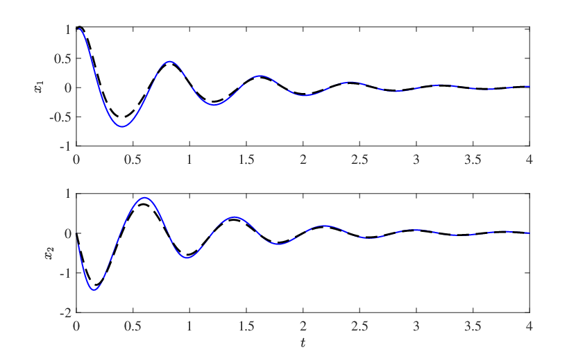
As these systems are unstable, for comparison purposes, the response of the nonlinear and the affine LPV system (with one scheduling variable) are computed under the same gain-scheduled state feedback controller. Fig. 3 reveals good coincidence between the time-domain simulation results starting from the initial state .
7 Experimental example
In this section, the proposed method is applied on a 3-DOF gyroscope system by Quanser, shown in Fig. 4. Using a first-principle model of the system and measured data, an LPV model of the system is constructed with our method. Subsequently, exploiting the obtained model, a full-order gain-scheduled output feedback controller is designed and applied on the setup. Converting the motion model of the gyroscope to an LPV form is challenging and results in an excessive number of scheduling variables Hoffmann and Werner 2015, so obtaining an LPV model with low number of scheduling variables is an achievement in itself by the proposed method.
7.1 Plant description
The gyroscope consists of a golden flywheel mounted inside an inner blue gimbal which in turn is mounted inside an outer red gimbal. The red gimbal is attached to a rotating silver frame. In the experiment considered in this paper, it is supposed that the rectangular silver frame is fixed. The blue and red gimbals can be actuated about their rotation axes using DC motors and the angular position of both gimbals are measured using optical encoders. The flywheel is actuated using another motor.
In our experiment, the flywheel is regulated by a controller which follows an unknown reference signal. The objective is to achieve servo control of the red and blue frames together by rejecting the disturbance generated by the change of the velocity of the flywheel. Let and represent the angular position of the blue and red gimbals, respectively. Moreover, the angular velocity of the flywheel, the blue gimbal, and the red gimbal are denoted by , , and . The torque applied on the blue and red gimbals are given by and .

7.2 LPV modeling
Through the Euler-Lagrange equations and frames defined for the rational bodies in the gyroscope, a dynamical motion model of the system is derived:
| (36) |
where is the inertia matrix and is the Coriolis matrix whose elements are derived as the result of the summation of the Christoffel symbols and the generalized angular velocities. The corresponding coefficients of these matrix functions are identified using measured data form the physical system and prediction error minimization with nonlinear optimization. As the flywheel can be seen as a separate subsystem, an NL-SS model of (36) w.r.t. the dynamics of the blue and red gimbals is derived in terms of (2) with
| (37) |
with and . Due to the division by to derive (37), the rather complicated rational trigonometrical expressions of which all depend on and also which depend on are not given here. The interested reader can obtain them from the equations provided in Bloemers and Toth 2019. (37) is a difficult nonlinear model for which we would like to obtain a low complexity affine LPV model (Problem 1). Using the proposed method with an affine LPV model is obtained:
| (38) | ||||
| (39) |
where . The corresponding matrices in the affine , , and the constant matrix are not included here for the sake of brevity. Moreover, the following bounds on the scheduling variables are obtained:
Additionally, one can readily compute the bounds on the derivative of the scheduling variables given below which are required for the controller synthesis in the next sections.
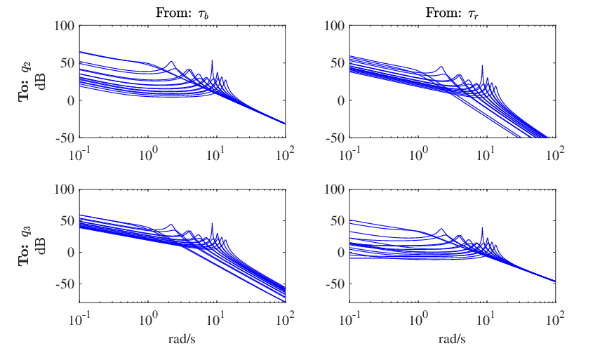
Thus, also lies in a hyper rectangle The quality of the obtained LPV model is assessed in a closed-loop simulation study with an LPV controller designed in Section 7.3 and compared with the closed loop response of the nonlinear system operated with the same controller. In case of the nonlinear gyroscope model, the angular velocity of the disc is regulated by a second controller to track a sinusoidal reference. Two multisine signals, different from those employed to obtain and construct , are used as the desired reference signals for and in the closed-loop simulation. The related results for , , , and are shown in Fig. 5. The root mean square error (RMSE) of the obtained response of the LPV model w.r.t. the true system response is given in Table 1. Obviously, the LPV model well captures the dynamics of the original system. Moreover, magnitude plots of the frequency response of the LPV model are depicted in Fig. 7 for some frozen scheduling variables in the related intervals, which clearly reveals the significant variation of the model over the scheduling set.



| RMSE | 0.0036 | 0.0049 | 0.0013 | 0.0029 |
7.3 Control synthesis
In this section, using the obtained LPV model in Section 7.2, a gain-scheduled full-order output feedback controller is sought for the gyroscope based on the closed-loop setup shown in Fig. 6. Roughly speaking, the -type performance, more precisely the induced -gain performance, is considered to shape the frozen sensitivity and control sensitivity functions of the feedback system. To obtain good tracking performance, while the actuator constraints are taken into account, the following weighting functions are employed:
The weighting function has been designed based on the standard mixed-sensitivity shaping approach to shape the frozen sensitivity frequency responses of the closed-loop system. is chosen such that corresponds to a low-pass filter with bandwidth 0.7 rad/s and low frequency gain of about 80 dB to ensure good disturbance attenuation, fast response time and less than 20% of expected overshoot. Similarly the control sensitivity weighting function, , has been chosen considering the amplitude and frequency constraints on the voltage to be applied to the DC motors of the experimental setup. The open-loop weighted plant displayed in Fig. 6 (by removing the controller) can be expressed as:
| (40) | ||||
where , , , , and respectively denote the state vector, the external input, the control input, the performance output, and the measured output of the system, with
| (41) |
where and are the state-space realizations of and , respectively.
The goal is to design the full-order gain-scheduled controller
such that it stabilizes the closed-loop system and assures an upper bound on the induced -gain performance. To design the controller, we use the method detailed in Sadeghzadeh 2018.
The resulting parameter-dependent LMI problems are solved through finite-dimensional LMI relaxation exploiting homogeneous polynomial matrices inspired by the method of Oliveira and Peres 2007. To this end, YALMIP Löfberg 2004 and ROLMIP Agulhari et al. 2012 interfaces for the LMI solver MOSEK MOSEK ApS 2015 are employed. With a an 8th-order controller is obtained with a guaranteed -gain performance bound of .
7.4 Experimental results
In this section, the gain-scheduled controller designed based on the LPV model obtained via the proposed method in this paper is experimentally validated on the laboratory setup. The controller is described in block diagrams in MATLAB/Simulink. Then using a dSPACE board that implements a real time interface, it is applied on the setup. The angular velocity of the flywheel is made to track a sinusoidal reference between to rad/sec. Since the movements of blue and red gimbals do not considerably affect the rotational velocity of the flywheel, a simple proportional controller is employed to ensure the tracking. The change of the velocity of the flywheel is considered as the exogenous disturbance, and have to be rejected by the controller. The reference trajectories for gimbals blue and red, i.e. and , change within rad and are designed to cover different positions of blue and red gimbals with respect to each other. The desired and actual positions of the gimbals, the angular velocity of the flywheel, and the control input signals are shown in Fig. 8. One can see that both gimbals track successfully the related reference trajectories while the input torques and remain within acceptable levels.
8 Conclusion
A novel method taking advantage of PCA is devised in this paper for LPV embedding of nonlinear systems. Contrary to the available methods for LPV embedding of nonlinear models based on PCA, the PCA is applied on a data matrix consisting of the trajectories of all elements of the state-space matrices not solely the scheduling variables. Furthermore, by finding the minimum bounding box of the scheduling variables and its proper rotation, the conservativeness related to over bounding the admissible region of the scheduling variables is reduced by introducing an invertible transformation to find a new set of scheduling variables. In addition to academic examples, the proposed method is deployed to generate an LPV model for a 3-DOF gyroscope. Assessment of the LPV model and evaluation of the closed-loop performance, which is obtained by a designed gain-scheduled controller exploiting the developed LPV model, successfully demonstrate the applicability of the developed method in practice.
Acknowledgment
This work has received funding from the European Research Council (ERC) under the European Union’s Horizon 2020 research and innovation programme (grant agreement nr. 714663).
References
- Abbas et al. (2014) Abbas, H., Toth, R., Petreczky, M., Meskin, N., and Mohammadpour, J. (2014). Embedding of nonlinear systems in a linear parameter-varying representation. In Proceedings of the 19th IFAC World Congress of the International Federation of Automatic Control, (IFAC’14), 24-29 August 2014, Cape Town, South Africa, 6907–6913.
- Agulhari et al. (2012) Agulhari, C.M., de Oliveira, R.C.L.F., and Peres, P.L.D. (2012). Robust LMI Parser: a computational package to construct LMI conditions for uncertain systems. In XIX Brazilian Conference on Automation (CBA 2012), 2298–2305. Campina Grande, PB, Brazil.
- Bachnas et al. (2014) Bachnas, A.A., Tóth, R., Ludlage, J.H.A., and Mesbah, A. (2014). A review on data-driven linear parameter-varying modeling approaches: A high-purity distillation column case study. Journal of Process Control, 24(4), 272–285.
- Barequet and Har-Peled (2001) Barequet, G. and Har-Peled, S. (2001). Efficiently Approximating the Minimum-Volume Bounding Box of a Point Set in Three Dimensions. Journal of Algorithms, 38(1), 91–109.
- Bloemers and Toth (2019) Bloemers, T. and Toth, R. (2019). Equations of motion of a control moment gyroscope. Technical report, Eindhoven University of Technology.
- Caigny et al. (2008) Caigny, J.D., Camino, J.F., Oliveira, R.C.L.F., Peres, P.L.D., and Swevers, J. (2008). Gain-scheduled control of discrete-time polytopic time-varying systems. In Decision and Control, 2008. CDC 2008. 47th IEEE Conference on, 3872–3877.
- Daafouz et al. (2008) Daafouz, J., Bernussou, J., and Geromel, J.C. (2008). On Inexact LPV Control Design of Continuous-Time Polytopic Systems. IEEE Transactions on Automatic Control, 53(7), 1674–1678.
- Diener (2020) Diener, J. (2020). 2D minimal bounding box. URL \url{https://www.mathworks.com/matlabcentral/fileexchange/31126-2d-minimal-bounding-box}.
- Eckart and Young (1936) Eckart, C. and Young, G. (1936). The approximation of one matrix by another of lower rank. Psychometrika, 1(3), 211–218. 10.1007/BF02288367.
- Freeman and Shapira (1975) Freeman, H. and Shapira, R. (1975). Determining the minimum-area encasing rectangle for an arbitrary closed curve. Commun. ACM, 18(7), 409–413.
- Goos and Pintelon (2016) Goos, J. and Pintelon, R. (2016). Continuous-time identification of periodically parameter-varying state space models. Automatica, 71, 254 – 263.
- Hanema et al. (2019) Hanema, J., Lazar, M., and Tóth, R. (2019). Heterogeneously parameterized tube model predictive control for LPV systems. Automatica, 111, 1–13.
- Hjartarson et al. (2015) Hjartarson, A., Seiler, P., and Packard, A. (2015). LPVTools: A toolbox for modeling, analysis, and synthesis of parameter varying control systems. In Proc. of the 1st IFAC Workshop on Linear Parameter Varying Systems, 139–145. Grenoble, France.
- Hoffmann and Werner (2015) Hoffmann, C. and Werner, H. (2015). Compact LFT-LPV modeling with automated parameterization for efficient LPV controller synthesis. In 2015 American Control Conference (ACC), 119–124.
- Hoffmann and Werner (2015) Hoffmann, C. and Werner, H. (2015). LFT-LPV modeling and control of a control moment gyroscope. In Proc. of the 54th IEEE Conference on Decision and Control, 5328–5333. Osaka, Japan.
- Hoffmann and Werner (2015) Hoffmann, C. and Werner, H. (2015). A survey of linear parameter-varying control applications validated by experiments or high-fidelity simulations. IEEE Transactions on Control Systems Technology, 23(2), 416–433.
- Kabsch (1976) Kabsch, W. (1976). A solution for the best rotation to relate two sets of vectors. Acta Crystallographica Section A, 32(5), 922–923.
- Khachiyan (1996) Khachiyan, L.G. (1996). Rounding of polytopes in the real number model of computation. Mathematics of Operations Research, 21(2), 307–320.
- Korsawe (2020) Korsawe, J. (2020). Minimal bounding box. URL \url{https://www.mathworks.com/matlabcentral/fileexchange/18264-minimal-bounding-box}.
- Kumar and Yildirim (2005) Kumar, P. and Yildirim, E.A. (2005). Minimum-Volume Enclosing Ellipsoids and Core Sets. Journal of Optimization Theory and Applications, 126(1), 1–21.
- Kwiatkowski and Werner (2008) Kwiatkowski, A. and Werner, H. (2008). PCA-based parameter set mappings for LPV models with fewer parameters and less overbounding. IEEE Transactions on Control Systems Technology, 16(4), 781–788.
- Laurain et al. (2012) Laurain, V., Tóth, R., Zheng, W.X., and Gilson, M. (2012). Nonparametric identification of lpv models under general noise conditions: An ls-svm based approach. IFAC Proceedings Volumes, 45(16), 1761 – 1766. https://doi.org/10.3182/20120711-3-BE-2027.00230. URL http://www.sciencedirect.com/science/article/pii/S1474667015382112. 16th IFAC Symposium on System Identification.
- Leith and Leithhead (1998) Leith, D.J. and Leithhead, W.E. (1998). Gain-scheduled nonlinear systems: Dynamic analysis by velocity based linearization families. Int. Journal of Control, 70, 289–317.
- Liu et al. (2019) Liu, X., Yang, X., Zhu, P., and Wang, Y. (2019). Robust multimodel identification of LPV systems with missing observations based on t-distribution. IEEE Transactions on Systems, Man, and Cybernetics: Systems, 1–7.
- Löfberg (2004) Löfberg, J. (2004). YALMIP: A Toolbox for Modeling and Optimization in MATLAB. In CACSD Conference.
- Marcos and Balas (2004) Marcos, A. and Balas, G.J. (2004). Development of linear-parameter-varying models for aircraft. Journal of Guidance, Control and Dynamics, 27(2), 218–228.
- MOSEK ApS (2015) MOSEK ApS (2015). The MOSEK optimization toolbox for MATLAB manual. Version 7.1 (Revision 28). URL http://docs.mosek.com/7.1/toolbox/index.html.
- Moshtagh (2020) Moshtagh, N. (2020). Minimum volume enclosing ellipsoid. URL \url{https://www.mathworks.com/matlabcentral/fileexchange/9542-minimum-volume-enclosing-ellipsoid}.
- Oliveira and Peres (2007) Oliveira, R.C.L.F. and Peres, P.L.D. (2007). Parameter-Dependent LMIs in Robust Analysis: Characterization of Homogeneous Polynomially Parameter-Dependent Solutions Via LMI Relaxations. IEEE Transactions on Automatic Control, 52(7), 1334–1340.
- Olver and Shakiban (2006) Olver, P.J. and Shakiban, C. (2006). Applied Linear Algebra. Prentice-Hall, Englewood Cliffs, NY.
- O’Rourke (1985) O’Rourke, J. (1985). Finding minimal enclosing boxes. International Journal of Computer & Information Sciences, 14(3), 183–199.
- Robles et al. (2019) Robles, R., Sala, A., and Bernal, M. (2019). Performance-oriented quasi-LPV modeling of nonlinear systems. International Journal of Robust and Nonlinear Control, 29(5), 1230–1248.
- Rugh and Shamma (2000a) Rugh, W. and Shamma, J.S. (2000a). Research on gain scheduling. Automatica, 36(10), 1401–1425.
- Rugh and Shamma (2000b) Rugh, W.J. and Shamma, J.S. (2000b). Research on gain scheduling. Automatica, 36(10), 1401–1425.
- Sadeghzadeh (2019) Sadeghzadeh, A. (2019). LMI relaxations for robust gain-scheduled control of uncertain linear parameter varying systems. IET Control Theory Applications, 13(4), 486–495.
- Sadeghzadeh (2018) Sadeghzadeh, A. (2018). Gain-scheduled continuous-time control using polytope-bounded inexact scheduling parameters. International Journal of Robust and Nonlinear Control, 28(17), 5557–5574.
- Sato and Peaucelle (2013) Sato, M. and Peaucelle, D. (2013). Gain-scheduled output-feedback controllers using inexact scheduling parameters for continuous-time LPV systems. Automatica, 49(4), 1019–1025.
- Scherer (2001) Scherer, C.W. (2001). LPV control and full block multipliers. Automatica, 37(3), 361–375.
- Schoukens and Toth (2018) Schoukens, M. and Toth, R. (2018). Linear parameter varying representation of a class of mimo nonlinear systems. IFAC-PapersOnLine, 51(26), 94 – 99. 2nd IFAC Workshop on Linear Parameter Varying Systems LPVS 2018.
- Shin et al. (2002) Shin, J.Y., Balas, G., and Kaya, M.A. (2002). Blending methodology of linear parameter varying control synthesis of F-16 aircraft system. Journal of Guidance, Control, and Dynamics, 25(6), 1040–1048.
- Siraj et al. (2012) Siraj, M.M., Tóth, R., and Weiland, S. (2012). Joint order and dependency reduction for lpv state-space models. In 2012 IEEE 51st IEEE Conference on Decision and Control (CDC), 6291–6296.
- Todd and Yıldırım (2007) Todd, M.J. and Yıldırım, E.A. (2007). On khachiyan’s algorithm for the computation of minimum-volume enclosing ellipsoids. Discrete Applied Mathematics, 155(13), 1731 – 1744.
- Toth (2010) Toth, R. (2010). Modeling and identification of linear parameter-varying systems. Lecture notes in control and information sciences. Springer, Germany. 10.1007/978-3-642-13812-6.
- Tóth et al. (2012) Tóth, R., Heuberger, P.S.C., and Van den Hof, P.M.J. (2012). Prediction-Error Identification of LPV Systems: Present and Beyond, 27–58. Springer US, Boston, MA.
- Toussaint (1983) Toussaint, G. (1983). Solving geometric problems with the rotating calipers. In IEEE Mediterranean Electronical Conference.
- Tóth et al. (2012) Tóth, R., Laurain, V., Gilson, M., and Garnier, H. (2012). Instrumental variable scheme for closed-loop LPV model identification. Automatica, 48(9), 2314 – 2320.
- Zhao et al. (2012) Zhao, Y., Huang, B., Su, H., and Chu, J. (2012). Prediction error method for identification of LPV models. Journal of Process Control, 22(1), 180 – 193.
- Zin et al. (2006) Zin, A., Sename, O., Gáspár, P., Dugard, L., and Bokor, J. (2006). An lpv/ active suspension control for global chassis technology: Design and performance analysis. In Proc. of the American Control Conference, 2945–2950.