跳到论文正文
W Papers独立论文阅读器 arXiv:2010.01489 论文正文 计算阅读时间 · 0%
引用这篇论文根据当前论文元数据生成,正式投稿前建议核对。


License: arXiv.org perpetual non-exclusive license
arXiv:2010.01489v1 [astro-ph.HE] 04 Oct 2020

Gravito-magnetic instabilities of Relativistic Magnetohydrodynamics

Hyerim Noh1,2, Jai-chan Hwang2,3 Address: 1Center for Large Telescope, Korea Astronomy and Space Science Institute, Daejon, Korea
2Kavli Institute for Cosmology Cambridge, Madingley Road, Cambridge CB3 0HA, United Kingdom
3Department of Astronomy and Atmospheric Sciences, Kyungpook National University, Daegu, Korea
Abstract

We study gravito-magnetic instabilities of a static homogeneous medium with an aligned magnetic field in the two contexts of relativistic magnetohydrodynamics (MHD): first, MHD with post-Newtonian (PN) corrections, and second, special relativistic (SR) MHD with weak gravity. The analysis in the PN MHD is made without taking the temporal gauge condition, thus results are gauge-invariant. The PN corrections of the internal energy, pressure, sound velocity and the Alfvén velocity lower the critical (Jeans) wavelength. All relativistic effects tend to destabilize the system. Although the SR MHD with weak gravity is presented in the harmonic gauge, in the presence of gravity the stability analysis is strictly valid to Newtonian order. In the absence of gravity, the SR MHD is independent of the gauge condition. We present the plane wave velocities and the stability criteria in both cases.

Key words: gravitation - instabilities - magnetohydrodynamics (MHD) - relativistic processes - waves

I. Introduction

Recently we presented three formulations of the relativistic magnetohydrodynamics (MHD): (i) fully nonlinear and exact perturbation formulation of MHD in Einstein’s gravity, (ii) special relativistic (SR) MHD with weak (Newtonian) gravity, and (iii) MHD with first-order post-Newtonian (1PN) corrections; formulation (ii) is derived in the maximal slicing (temporal gauge or hypersurface) condition whereas formulations (i) and (iii) are presented without imposing the temporal gauge condition (Noh, Hwang & Bucher 2019; Hwang & Noh 2020). The SR MHD with weak gravity is complementary to the PN approximation: in the SR MHD with weak gravity the fluid and field are fully relativistic while the gravity is Newtonian, whereas in the PN MHD the the fluid, field and gravity are consistently weakly relativistic.

Previously we studied effects of 1PN corrections on the MHD waves in a static homogeneous medium with an aligned magnetic field (Hwang & Noh 2020). In this work we include the gravity for the same homogeneous medium and study the gravito-magnetic instability of the PN MHD and the SR MHD with weak gravity. Both formulations include the Newtonian (0PN) limit.

Gravitational instability is a major factor causing gravitational collapse to form celestial objects. Magnetic field ubiquitous in the universe affects the stability. The gravito-magnetic instability in Newtonian context was analyzed by Chandrasekhar & Fermi (1953) and Chandrasekhar (1954, 1961). Here our aim is to extend this Newtonian study to a couple of relativistic situations.

Besides (i) the 1PN destabilizing effects on the instability criteria stated in the abstract and (ii) waves and instability in the SR MHD with weak gravity, we address (iii) the issue of inconsistency surrounding the Poisson’s equation in the static homogeneous medium and (iv) the dependence of instability criteria on magnetic field to 0PN order.

Sections II and III are summaries of the MHD formulation to 1PN order, and the SR MHD with weak gravity. Section IV is the Newtonian (0PN) study of gravito-magnetic instability of homogeneous and static medium with a pressure and an aligned magnetic field. Sections V and VI are instabilities of the same medium extended to 1PN order and the SR MHD with weak gravity, respectively. Section VII is a summary of our results and Section VIII is a discussion. We take the cgs unit.

II. MHD formulation to 1PN order

We follow 1PN convention of Chandrasekhar (Chandrasekhar 1965; Chandrasekhar & Nutku 1969). The metric convention is

g~00=−{1−2c2​[U+1c2​(2​Υ−U2)]},\displaystyle\widetilde{g}_{00}=-\left\{1-{2\over c^{2}}\left[U+{1\over c^{2}}\left(2\Upsilon-U^{2}\right)\right]\right\},
g~0​i=−1c3​Pi,g~i​j=(1+2c2​V)​δi​j,\displaystyle\widetilde{g}_{0i}=-{1\over c^{3}}P_{i},\quad\widetilde{g}_{ij}=\left(1+{2\over c^{2}}V\right)\delta_{ij}, (1)

with V=UV=U; x0=c​tx^{0}=ct and a tilde indicates the covariant quantity; Υ\Upsilon is a pure 1PN order potential introduced in Chandrasekhar (1965), see our Equation (9). The energy momentum tensor is decomposed into fluid quantities as

T~a​b=μ~​u~a​u~a+p~​(g~a​b+u~a​u~b)+π~a​b,\displaystyle\widetilde{T}_{ab}=\widetilde{\mu}\widetilde{u}_{a}\widetilde{u}_{a}+\widetilde{p}\left(\widetilde{g}_{ab}+\widetilde{u}_{a}\widetilde{u}_{b}\right)+\widetilde{\pi}_{ab}, (2)
μ~≡μ≡ϱ​c2,ϱ≡ϱ¯​(1+1c2​Π),p~≡p,π~i​j≡Πi​j,\displaystyle\widetilde{\mu}\equiv\mu\equiv\varrho c^{2},\quad\varrho\equiv\overline{\varrho}\left(1+{1\over c^{2}}\Pi\right),\quad\widetilde{p}\equiv p,\quad\widetilde{\pi}_{ij}\equiv\Pi_{ij},

with fluid velocities viv_{i} and v¯i\overline{v}_{i}

u~i≡γ​vic,γ≡11−11+2​φ​v2c2,v2≡vi​vi;\displaystyle\widetilde{u}_{i}\equiv\gamma{v_{i}\over c},\quad\gamma\equiv{1\over\sqrt{1-{1\over 1+2\varphi}{v^{2}\over c^{2}}}},\quad v^{2}\equiv v^{i}v_{i};
v¯ic≡u~iu~0=d​xid​x0.\displaystyle{\overline{v}^{i}\over c}\equiv{\widetilde{u}^{i}\over\widetilde{u}^{0}}={dx^{i}\over dx^{0}}. (4)

For φ\varphi, see Equation (14). To 1PN order we have

vi=v¯i+1c2​(3​U​v¯i−Pi).\displaystyle v_{i}=\overline{v}_{i}+{1\over c^{2}}\left(3U\overline{v}_{i}-P_{i}\right). (5)

We will use v¯i\overline{v}_{i}. We are not imposing the temporal gauge condition which can be used as an advantage in handling problems. In our analysis of gravitational instability of PN MHD in Section V, in fact, we do not need to take the gauge condition. Thus, our results are valid in any temporal gauge condition.

A complete set of MHD equation valid to 1PN order is derived in Equations (53), (43), (56), (50), (49), (55), (54) and (48), respectively, in Hwang & Noh (2020) without imposing the temporal gauge condition. The mass, energy and momentum conservation equations are

∂∂t​[ϱ¯​(1+12​v2c2+3​Uc2)]\displaystyle{\partial\over\partial t}\left[\overline{\varrho}\left(1+{1\over 2}{v^{2}\over c^{2}}+3{U\over c^{2}}\right)\right]
+∇i[ϱ¯​v¯i​(1+12​v2c2+3​Uc2)]=0,\displaystyle\qquad+\nabla^{i}\left[\overline{\varrho}\overline{v}_{i}\left(1+{1\over 2}{v^{2}\over c^{2}}+3{U\over c^{2}}\right)\right]=0, (6)
ϱ¯(Π˙+𝐯⋅∇Π)+p∇⋅𝐯+Πi​jvi,j=0,\displaystyle\overline{\varrho}\left(\dot{\Pi}+{\bf v}\cdot\nabla\Pi\right)+p\nabla\cdot{\bf v}+\Pi^{ij}v_{i,j}=0, (7)
{ϱ¯+1c2[ϱ¯(Π+v2+6U)+p]}(v¯˙i+𝐯¯⋅∇𝐯¯𝐢)+p,i\displaystyle\left\{\overline{\varrho}+{1\over c^{2}}\left[\overline{\varrho}\left(\Pi+v^{2}+6U\right)+p\right]\right\}\left(\dot{\overline{v}}_{i}+\overline{\bf v}\cdot\nabla\overline{v}_{i}\right)+p_{,i}
+Πi,jj+1c2[p˙vi+2p,iU+(Πi​jvj)⋅−vi(Πkjvk),j]\displaystyle\qquad+\Pi^{j}_{i,j}+{1\over c^{2}}\left[\dot{p}v_{i}+2p_{,i}U+\left(\Pi_{ij}v^{j}\right)^{\displaystyle{\cdot}}-v_{i}\left(\Pi^{j}_{k}v^{k}\right)_{,j}\right]
−{ϱ¯+1c2[ϱ¯(Π+2v2+2U)+p]}U,i−1c22ϱ¯Υ,i\displaystyle\qquad-\left\{\overline{\varrho}+{1\over c^{2}}\left[\overline{\varrho}\left(\Pi+2v^{2}+2U\right)+p\right]\right\}U_{,i}-{1\over c^{2}}2\overline{\varrho}\Upsilon_{,i}
+1c2​ϱ¯​[(3​U˙+4​𝐯⋅∇U)​vi−P˙i−vj​(Pi,j−Pj,i)]\displaystyle\qquad+{1\over c^{2}}\overline{\varrho}\left[\left(3\dot{U}+4{\bf v}\cdot\nabla U\right)v_{i}-\dot{P}_{i}-v^{j}\left(P_{i,j}-P_{j,i}\right)\right]
=14​π​[(∇×𝐁)×𝐁]i\displaystyle\qquad={1\over 4\pi}\left[\left(\nabla\times{\bf B}\right)\times{\bf B}\right]_{i}
+14​π​c2{[(𝐯×𝐁)⋅×𝐁]i+(𝐯×𝐁)i∇⋅(𝐯×𝐁)\displaystyle\qquad+{1\over 4\pi c^{2}}\Big\{\left[\left({\bf v}\times{\bf B}\right)^{\displaystyle{\cdot}}\times{\bf B}\right]_{i}+\left({\bf v}\times{\bf B}\right)_{i}\nabla\cdot\left({\bf v}\times{\bf B}\right)
+vi(𝐯×𝐁)⋅(∇×𝐁)−[𝐁×(𝐁×∇U)]i}.\displaystyle\qquad+v_{i}\left({\bf v}\times{\bf B}\right)\cdot\left(\nabla\times{\bf B}\right)-\left[{\bf B}\times\left({\bf B}\times\nabla U\right)\right]_{i}\Big\}. (8)

Einstein equations are

ΔU+4πGϱ¯=−1c2[2ΔΥ+3U¨+P˙,kk\displaystyle\Delta U+4\pi G\overline{\varrho}=-{1\over c^{2}}\bigg[2\Delta\Upsilon+3\ddot{U}+\dot{P}^{k}_{\;\;,k}
+4πGϱ¯(Π+2v2+3pϱ¯+2U+B24​π​ϱ¯)],\displaystyle\qquad+4\pi G\overline{\varrho}\left(\Pi+2v^{2}+3{p\over\overline{\varrho}}+2U+{B^{2}\over 4\pi\overline{\varrho}}\right)\bigg], (9)
ΔPi−(P,kk+4U˙),i=−16πGϱ¯vi.\displaystyle\Delta P_{i}-\left(P^{k}_{\;\;,k}+4\dot{U}\right)_{,i}=-16\pi G\overline{\varrho}v_{i}. (10)

The Maxwell’s equations are

∂∂t​[(1+Uc2)​𝐁]=∇×[(1+Uc2)​𝐯¯×𝐁].\displaystyle{\partial\over\partial t}\left[\left(1+{U\over c^{2}}\right){\bf B}\right]=\nabla\times\left[\left(1+{U\over c^{2}}\right)\overline{\bf v}\times{\bf B}\right]. (11)
∇⋅[(1+Uc2)​𝐁]=0,\displaystyle\nabla\cdot\left[\left(1+{U\over c^{2}}\right){\bf B}\right]=0, (12)

Equations (6)-(12) are the complete set of MHD equations valid to 1PN order without imposing the temporal gauge condition.

The general slicing condition to the 1PN order is

Pi,i+nU˙=0,\displaystyle P^{i}_{\;\;,i}+n\dot{U}=0, (13)

where n=3n=3 and 44 correspond to the Chandrasekhar (Standard PN) gauge (Greenberg 1971) and the harmonic gauge (Nazari & Roshan 2018), respectively (Hwang, Noh & Puetzfeld 2008; Poisson & Will 2014).

Equation (10) applies only to the 1PN order. Spatial indices of the fluid (viv_{i}, v¯i\overline{v}_{i}, Πi​j\Pi_{ij}), field (BiB_{i}) and the metric (PiP_{i}) variables are raised and lowered using δi​j\delta_{ij} and its inverse metric.

III. SR MHD with weak gravity formulation

Our metric convention is

g~00=−(1+2​α),g~0​i=−χi,g~i​j=(1+2​φ)​δi​j,\displaystyle\widetilde{g}_{00}=-\left(1+2\alpha\right),\quad\widetilde{g}_{0i}=-\chi_{i},\quad\widetilde{g}_{ij}=\left(1+2\varphi\right)\delta_{ij},
(14)

where α\alpha, φ\varphi and χi\chi_{i} are functions of spacetime with arbitrary amplitudes. Fully nonlinear and exact perturbation formulation based on this metric is presented in the Appendix of Noh, Hwang & Bucher (2019).

Equations combining SR MHD with weak gravity are derived in Equations (3)-(5) and (10)-(14) in the same work, by assuming

α≡Φc2≪1,φ≡−Ψc2≪1,γ2​tℓ2tg2≪1,\displaystyle\alpha\equiv{\Phi\over c^{2}}\ll 1,\quad\varphi\equiv-{\Psi\over c^{2}}\ll 1,\quad\gamma^{2}{t_{\ell}^{2}\over t_{g}^{2}}\ll 1, (15)

where tg∼1/G​ϱt_{g}\sim 1/\sqrt{G\varrho} and tℓ∼ℓ/c∼2​π/(k​c)t_{\ell}\sim\ell/c\sim 2\pi/(kc) are gravitational timescale and the light propagation timescale of a characteristic length scale ℓ\ell, respectively; kk is the wave number with Δ=−k2\Delta=-k^{2}.

The mass, energy, and momentum conservation equations, and the two Maxwell equations, respectively, in conservative forms and Einstein’s equations are

∂∂t​(DEmiBi)+∇j(D​vjmj​c2mi​jvj​Bi−vi​Bj)\displaystyle{\partial\over\partial t}\left(\begin{array}[]{c}D\\ E\\ m^{i}\\ B^{i}\end{array}\right)+\nabla_{j}\left(\begin{array}[]{c}Dv^{j}\\ m^{j}c^{2}\\ m^{ij}\\ v^{j}B^{i}-v^{i}B^{j}\end{array}\right)
=(0−ϱ¯(2Φ−Ψ),ivi−ϱ¯Φ,i0),\displaystyle\qquad=\left(\begin{array}[]{c}0\\ -\overline{\varrho}\left(2\Phi-\Psi\right)_{,i}v^{i}\\ -\overline{\varrho}\Phi^{,i}\\ 0\end{array}\right),
Bi,i=0,\displaystyle B^{i}_{\;\;,i}=0, (30)
Δ​Φ=4​π​G​(ϱ+3​pc2+2c2​𝒮)=4​π​G​E+Sc2,\displaystyle\Delta\Phi=4\pi G\left(\varrho+{3p\over c^{2}}+{2\over c^{2}}{\cal S}\right)=4\pi G{E+S\over c^{2}}, (31)
Δ​Ψ=4​π​G​(ϱ+1c2​𝒮)=4​π​G​Ec2,\displaystyle\Delta\Psi=4\pi G\left(\varrho+{1\over c^{2}}{\cal S}\right)=4\pi G{E\over c^{2}}, (32)

where

D≡ϱ¯​γ,ϱ≡ϱ¯​(1+Πc2),γ=11−v2c2,\displaystyle D\equiv\overline{\varrho}\gamma,\quad\varrho\equiv\overline{\varrho}\left(1+{\Pi\over c^{2}}\right),\quad\gamma={1\over\sqrt{1-{v^{2}\over c^{2}}}},
E=ϱ​c2+𝒮,S=3​p+𝒮,𝒮≡(ϱ+pc2)​γ2​v2\displaystyle E=\varrho c^{2}+{\cal S},\quad S=3p+{\cal S},\quad{\cal S}\equiv\left(\varrho+{p\over c^{2}}\right)\gamma^{2}{v^{2}}
+Πi​j​vi​vjc2+18​π​[B2+1c2​(𝐯×𝐁)2],\displaystyle\qquad+\Pi_{ij}{v^{i}v^{j}\over c^{2}}+{1\over 8\pi}\left[B^{2}+{1\over c^{2}}\left({\bf v}\times{\bf B}\right)^{2}\right],
mi≡(ϱ+pc2)​γ2​vi\displaystyle m^{i}\equiv\left(\varrho+{p\over c^{2}}\right)\gamma^{2}v^{i}
+1c2​[Πji​vj+14​π​(B2​vi−Bi​Bj​vj)],\displaystyle\qquad+{1\over c^{2}}\left[\Pi^{i}_{j}v^{j}+{1\over 4\pi}\left(B^{2}v^{i}-B^{i}B^{j}v_{j}\right)\right],
mi​j≡(ϱ+pc2)​γ2​vi​vj+p​δi​j+Πi​j\displaystyle m^{ij}\equiv\left(\varrho+{p\over c^{2}}\right)\gamma^{2}v^{i}v^{j}+p\delta^{ij}+\Pi^{ij}
+14​π{1γ2(12B2δi​j−BiBj)+1c2[B2vivj\displaystyle\qquad+{1\over 4\pi}\bigg\{{1\over\gamma^{2}}\left({1\over 2}B^{2}\delta^{ij}-B^{i}B^{j}\right)+{1\over c^{2}}\bigg[B^{2}v^{i}v^{j}
+12(Bkvk)2δi​j−(Bjvi+Bivj)Bkvk]}.\displaystyle\qquad+{1\over 2}\left(B^{k}v_{k}\right)^{2}\delta^{ij}-\left(B^{j}v^{i}+B^{i}v^{j}\right)B^{k}v_{k}\bigg]\bigg\}. (33)

The remaining metric component χi\chi_{i} is determined by

Δ​χi=−4​π​Gc3​(4​δij−Δ−1​∇i∇j)​mj.\displaystyle\Delta\chi_{i}=-{4\pi G\over c^{3}}\left(4\delta_{i}^{j}-\Delta^{-1}\nabla_{i}\nabla^{j}\right)m_{j}. (34)

Indices of χi\chi_{i}, mim_{i} and mi​jm_{ij} are raised and lowered using δi​j\delta_{ij} and its inverse.

The SR MHD with weak gravity formulation is valid in the maximal slicing (the uniform-expansion gauge in cosmology), setting the trace of extrinsic curvature (expansion scalar of the normal frame with a minus sign) equal to zero, which corresponds to the harmonic gauge in the PN approximation. If we ignore gravity, the SR MHD is valid in the Minkowski background, thus independent of the gauge condition. We have derived the formulation from the fully nonlinear an exact perturbation formulation of Einstein’s gravity by taking the limit in Equation (15). We note that when we consider the conservation equations, in strict sense of the limit used in Equation (15) the gravity part is valid only to the Newtonian order, thus we have Ψ=Φ=−U\Psi=\Phi=-U and Δ​Φ=4​π​G​ϱ¯\Delta\Phi=4\pi G\overline{\varrho} (Noh, Hwang & Bucher 2019). We have vi=v¯iv_{i}=\overline{v}_{i}.

IV. Stability to 0PN order

To the 0PN order, Equations (6)-(12) give

ϱ¯˙+∇⋅(ϱ¯​𝐯)=0,\displaystyle\dot{\overline{\varrho}}+\nabla\cdot\left(\overline{\varrho}{\bf v}\right)=0, (35)
ϱ¯(𝐯˙+𝐯⋅∇𝐯)+∇p+∇jΠij−ϱ¯∇U\displaystyle\overline{\varrho}\left(\dot{\bf v}+{\bf v}\cdot\nabla{\bf v}\right)+\nabla p+\nabla_{j}\Pi^{j}_{i}-\overline{\varrho}\nabla U
=14​π​(∇×𝐁)×𝐁,\displaystyle\qquad={1\over 4\pi}\left(\nabla\times{\bf B}\right)\times{\bf B}, (36)
Δ​U=−4​π​G​ϱ¯,\displaystyle\Delta U=-4\pi G\overline{\varrho}, (37)
𝐁˙=∇×(𝐯×𝐁),\displaystyle\dot{\bf B}=\nabla\times\left({\bf v}\times{\bf B}\right), (38)
∇⋅𝐁=0.\displaystyle\nabla\cdot{\bf B}=0. (39)

For our stability analysis we do not need the energy conservation equation in (7) which is in fact 1PN order (Hwang & Noh 2013). In this work we ignore the anisotropic stress. The above equations also follow from Equations (III)-(32) by taking cc-goes-to-infinite limit with Φ=Ψ=−U\Phi=\Psi=-U.

We consider a static homogeneous background with a uniform magnetic field (Chandrasekhar & Fermi 1953; Chandrasekhar 1954, 1961). To the background order, we have a solution with

ϱ¯0=constant,p0=constant,𝐯0=0,\displaystyle\overline{\varrho}_{0}={\rm constant},\quad p_{0}={\rm constant},\quad{\bf v}_{0}=0,
𝐁0=B0​𝐧=constant,|𝐧|=1,∇U0=0,\displaystyle{\bf B}_{0}=B_{0}{\bf n}={\rm constant},\quad|{\bf n}|=1,\quad\nabla U_{0}=0, (40)

but Δ​U0=−4​π​G​ϱ¯0\Delta U_{0}=-4\pi G\overline{\varrho}_{0}.

Notice the inconsistent relations involving U0U_{0}. The trouble is caused because we consider Minkowski (thus static) background despite the presence of self gravity of an infinite homogeneous background. The inconsistency is naturally avoided in the relativistic study of dynamic background as in the case of cosmology: the background order density, ϱ0\varrho_{0}, is absorbed into the background (Friedmann) equations, and the Poisson’s equation is valid only to perturbed order, thus U=δ​UU=\delta U without U0U_{0}, see Equations (85)-(88), (108) and (119) in Hwang, Noh & Puetzfeld (2008). In the static background, as in the present case, however, the inconsistency (often known as a swindle) remains. Jeans has made an explicit choice of ignoring the inconsistency, see Section 46 of Jeans (1902). Although the U0U_{0} term does not appear in perturbation analysis to 0PN order, it appears in the perturbation equations to the 1PN order, see Equations (64)-(71). See a paragraph below Equation (71) for further discussion.

Considering the linear order perturbation, we expand

ϱ¯=ϱ¯0​(1+δ),p=p0+δ​p,𝐁=𝐁0+δ​𝐁,\displaystyle\overline{\varrho}=\overline{\varrho}_{0}\left(1+\delta\right),\quad p=p_{0}+\delta p,\quad{\bf B}={\bf B}_{0}+\delta{\bf B},
𝐯=δ​𝐯,U=U0+δ​U,\displaystyle{\bf v}=\delta{\bf v},\quad U=U_{0}+\delta U, (41)

and introduce

δ​p≡cs2​ϱ¯0​δ,cA2≡B024​π​ϱ¯0,δ​𝐁≡B0​𝐛,\displaystyle\delta p\equiv c_{s}^{2}\overline{\varrho}_{0}\delta,\quad c_{A}^{2}\equiv{B_{0}^{2}\over 4\pi\overline{\varrho}_{0}},\quad\delta{\bf B}\equiv B_{0}{\bf b}, (42)

with the adiabatic sound speed cs=constantc_{s}={\rm constant}; thus, we are considering a barotropic equation of state with p=p⁡(ϱ¯)p=p(\overline{\varrho}). Equations (35)-(39) give

δ˙=−∇⋅𝐯,\displaystyle\dot{\delta}=-\nabla\cdot{\bf v}, (43)
𝐯˙+cs2∇δ−∇δU=cA2[∇(𝐧⋅𝐛)−𝐧⋅∇𝐛],\displaystyle\dot{\bf v}+c_{s}^{2}\nabla\delta-\nabla\delta U=c_{A}^{2}\left[\nabla\left({\bf n}\cdot{\bf b}\right)-{\bf n}\cdot\nabla{\bf b}\right], (44)
Δ​δ​U=−4​π​G​ϱ¯0​δ,\displaystyle\Delta\delta U=-4\pi G\overline{\varrho}_{0}\delta, (45)
𝐛˙=𝐧⋅∇𝐯−𝐧∇⋅𝐯,\displaystyle\dot{\bf b}={\bf n}\cdot\nabla{\bf v}-{\bf n}\nabla\cdot{\bf v}, (46)
∇⋅𝐛=0.\displaystyle\nabla\cdot{\bf b}=0. (47)

Expanding the perturbations in plane waves proportional to ei⁡(𝐤⋅𝐱−ω​t)e^{i({\bf k}\cdot{\bf x}-\omega t)}, we have

[ω2−cA2(𝐧⋅𝐤)2]𝐯+[(4​π​G​ϱ¯0k2−cs2−cA2)𝐤\displaystyle\left[\omega^{2}-c_{A}^{2}\left({\bf n}\cdot{\bf k}\right)^{2}\right]{\bf v}+\bigg[\left({4\pi G\overline{\varrho}_{0}\over k^{2}}-c_{s}^{2}-c_{A}^{2}\right){\bf k}
+cA2𝐧𝐧⋅𝐤]𝐤⋅𝐯+cA2𝐤𝐤⋅𝐧𝐧⋅𝐯=0.\displaystyle\qquad+c_{A}^{2}{\bf n}{\bf n}\cdot{\bf k}\bigg]{\bf k}\cdot{\bf v}+c_{A}^{2}{\bf k}{\bf k}\cdot{\bf n}{\bf n}\cdot{\bf v}=0. (48)

By introducing coordinates as (Shu 1992)

𝐤≡k​𝐱^,𝐧≡cos⁡ψ​𝐱^+sin⁡ψ​𝐲^,𝐯≡vx​𝐱^+vy​𝐲^+vz​𝐳^,\displaystyle{\bf k}\equiv k\widehat{\bf x},\quad{\bf n}\equiv\cos{\psi}\widehat{\bf x}+\sin{\psi}\widehat{\bf y},\quad{\bf v}\equiv v_{x}\widehat{\bf x}+v_{y}\widehat{\bf y}+v_{z}\widehat{\bf z},
(49)

Equations (43), (46) and (47) give vx=(ω/k)​δv_{x}=(\omega/k)\delta, bx=0b_{x}=0,

by=kω​(sin⁡ψ​vx−cos⁡ψ​vy),bz=−kω​cos⁡ψ​vz,\displaystyle b_{y}={k\over\omega}\left(\sin{\psi}v_{x}-\cos{\psi}v_{y}\right),\quad b_{z}=-{k\over\omega}\cos{\psi}v_{z}, (50)

and Equation (48) gives

[ω2+k2​(4​π​G​ϱ¯0k2−cs2−cA2​sin2⁡ψ)]​vx\displaystyle\left[\omega^{2}+k^{2}\left({4\pi G\overline{\varrho}_{0}\over k^{2}}-c_{s}^{2}-c_{A}^{2}\sin^{2}{\psi}\right)\right]v_{x}
+k2​cA2​sin⁡ψ​cos⁡ψ​vy=0,\displaystyle\qquad+k^{2}c_{A}^{2}\sin{\psi}\cos{\psi}v_{y}=0, (51)
k2​cA2​cos⁡ψ​sin⁡ψ​vx+(ω2−k2​cA2​cos2⁡ψ)​vy=0,\displaystyle k^{2}c_{A}^{2}\cos{\psi}\sin{\psi}v_{x}+\left(\omega^{2}-k^{2}c_{A}^{2}\cos^{2}{\psi}\right)v_{y}=0, (52)
(ω2−k2​cA2​cos2⁡ψ)​vz=0.\displaystyle\left(\omega^{2}-k^{2}c_{A}^{2}\cos^{2}{\psi}\right)v_{z}=0. (53)

For vz≠0v_{z}\neq 0 (𝐯{\bf v} perpendicular to 𝐁0{\bf B}_{0}-𝐤{\bf k} plane), Equation (53) gives

ω2k2=cA2​cos2⁡ψ.\displaystyle{\omega^{2}\over k^{2}}=c_{A}^{2}\cos^{2}{\psi}. (54)

For non-vanishing vxv_{x} and vyv_{y} (𝐯{\bf v} in 𝐁0{\bf B}_{0}-𝐤{\bf k} plane), from Equations (51) and (52) we have a dispersion relation

ω4+[4​π​G​ϱ¯0−k2​(cs2+cA2)]​ω2\displaystyle\omega^{4}+\left[4\pi G\overline{\varrho}_{0}-k^{2}\left(c_{s}^{2}+c_{A}^{2}\right)\right]\omega^{2}
+cA2​(k2​cs2−4​π​G​ϱ¯0)​(𝐤⋅𝐧)2=0,\displaystyle\qquad+c_{A}^{2}\left(k^{2}c_{s}^{2}-4\pi G\overline{\varrho}_{0}\right)\left({\bf k}\cdot{\bf n}\right)^{2}=0, (55)

with two solutions

ω2k2=12{cs2+cA2−4​π​G​ϱ¯0k2±[(cs2+cA2−4​π​G​ϱ¯0k2)2\displaystyle{\omega^{2}\over k^{2}}={1\over 2}\bigg\{c_{s}^{2}+c_{A}^{2}-{4\pi G\overline{\varrho}_{0}\over k^{2}}\pm\bigg[\left(c_{s}^{2}+c_{A}^{2}-{4\pi G\overline{\varrho}_{0}\over k^{2}}\right)^{2}
−4cA2(cs2−4​π​G​ϱ¯0k2)(𝐤⋅𝐧)2k2]1/2}.\displaystyle\qquad-4c_{A}^{2}\left(c_{s}^{2}-{4\pi G\overline{\varrho}_{0}\over k^{2}}\right){({\bf k}\cdot{\bf n})^{2}\over k^{2}}\bigg]^{1/2}\bigg\}. (56)

Equation (55) was presented in Equation (169) of Chandrasekhar & Fermi (1953). Behavior of the solutions are presented in Figure 1.

Refer to caption
Figure 1.— Behaviors of two solutions in Equation (56) with the upper (plus) and lower (minus) signs in dotted and solid lines, respectively. The xx-axis is kk in the unit of kJk_{J} and the yy-axis is ω2\omega^{2} in the unit of 4​π​G​ϱ¯04\pi G\overline{\varrho}_{0}. The red, cyan, magenta and blue indicate ψ=0o\psi=0^{\rm o}, 45o45^{\rm o}, 80o80^{\rm o} and 90o90^{\rm o}, respectively. From left to right are for s≡cA2/cs2=0.5s\equiv c_{A}^{2}/c_{s}^{2}=0.5, 11 and 22, respectively. The lower graphs are the same behaviors using ω2/|ω|\omega^{2}/|\omega| for yy-axis; these correspond to Figure 136 in Chandrasekhar (1961).

For 𝐤|𝐁0{\bf k}\parallel{\bf B}_{0} (ψ=0o\psi=0^{\rm o}), we have

ω2k2=cs2−4​π​G​ϱ¯0k2,cA2,\displaystyle{\omega^{2}\over k^{2}}=c_{s}^{2}-{4\pi G\overline{\varrho}_{0}\over k^{2}},\quad c_{A}^{2}, (57)

with the faster (slower) mode the fast (slow) MHD waves in the absence of gravity (Shu 1992). In the presence of gravity one mode is unstable for k<kJk<k_{J} with the Jeans wavenumber given as

kJ2=4​π​G​ϱ¯0cs2,\displaystyle k^{2}_{J}={4\pi G\overline{\varrho}_{0}\over c_{s}^{2}}, (58)

which does not depend on the magnetic field as pointed out in Chandrasekhar & Fermi (1953); for example, Chandrasekhar (1954) mentions “Jeans’s criterion for the gravitational instability of an infinite homogeneous medium is unaffected by the presence of a magnetic field.”; however, this is not a generally valid conclusion as we show below.

For 𝐤⟂𝐁0{\bf k}\perp{\bf B}_{0} (ψ=90o\psi=90^{\rm o}), we have

ω2k2=(cs2+cA2)−4​π​G​ϱ¯0k2,0,\displaystyle{\omega^{2}\over k^{2}}=\left(c_{s}^{2}+c_{A}^{2}\right)-{4\pi G\overline{\varrho}_{0}\over k^{2}},\quad 0, (59)

with the fast mode the magnetosonic wave in the absence of gravity (Shu 1992) and the slow mode vanishing. In the presence of gravity one mode is unstable for k<kBk<k_{B} with the critical wavenumber modified as

kB2=4​π​G​ϱ¯0cs2+cA2,\displaystyle k^{2}_{B}={4\pi G\overline{\varrho}_{0}\over c_{s}^{2}+c_{A}^{2}}, (60)

thus depends on the magnetic field with kB<kJk_{B}<k_{J} (Pacholczyk & Stodółkiewicz 1960; Strittmatter 1966).

For ψ\psi other than 90o90^{\rm o}, the stability criterion remains the same as the Jeans criterion in Equation (58). However, as Figure 1 shows, the instability for kB<k<kJk_{B}<k<k_{J} is suppressed depending on ψ\psi, and as ψ\psi approaches 90o90^{\rm o} the stability criterion effectively becomes Equation (60).

V. Stability to 1PN order

We similarly consider a static homogeneous background without anisotropic stress. To the background order, we have a solution with

ϱ¯0=constant,Π0=constant,p0=constant,\displaystyle\overline{\varrho}_{0}={\rm constant},\quad\Pi_{0}={\rm constant},\quad p_{0}={\rm constant},
𝐯0=0=𝐯¯𝟎,𝐁𝟎=𝐁𝟎​𝐧=constant,\displaystyle{\bf v}_{0}=0=\overline{\bf v}_{0},\hskip 11.49994pt{\bf B}_{0}=B_{0}{\bf n}={\rm constant},
∇U0=0=U˙0,∇Υ0=0,𝐏0=0,\displaystyle\nabla U_{0}=0=\dot{U}_{0},\quad\nabla\Upsilon_{0}=0,\quad{\bf P}_{0}=0, (61)

but we have

ΔU0+4πGϱ¯0=−1c2[2ΔΥ0\displaystyle\Delta U_{0}+4\pi G\overline{\varrho}_{0}=-{1\over c^{2}}\big[2\Delta\Upsilon_{0}
+4πGϱ¯0(Π0+2U0)+12πGp0+GB02],\displaystyle\qquad+4\pi G\overline{\varrho}_{0}\left(\Pi_{0}+2U_{0}\right)+12\pi Gp_{0}+GB_{0}^{2}\big], (62)

with Δ​U0≠0≠Δ​Υ0\Delta U_{0}\neq 0\neq\Delta\Upsilon_{0}. Thus, the inconsistent relations involving U0U_{0} and Υ0\Upsilon_{0} continue to 1PN order, see a paragraph below Equation (71). We consider p0p_{0} and Π0\Pi_{0} as constants in space and time.

To the linear order perturbation, we expand

ϱ¯=ϱ¯0​(1+δ),Π=Π0+δ​Π,p=p0+δ​p,\displaystyle\overline{\varrho}=\overline{\varrho}_{0}\left(1+\delta\right),\quad\Pi=\Pi_{0}+\delta\Pi,\quad p=p_{0}+\delta p,
𝐁=𝐁0+δ​𝐁,𝐯=δ​𝐯,𝐯¯=δ​𝐯¯,\displaystyle{\bf B}={\bf B}_{0}+\delta{\bf B},\quad{\bf v}=\delta{\bf v},\quad\overline{\bf v}=\delta\overline{\bf v},
U=U0+δ​U,Υ=Υ0+δ​Υ,𝐏=δ​𝐏.\displaystyle U=U_{0}+\delta U,\quad\Upsilon=\Upsilon_{0}+\delta\Upsilon,\quad{\bf P}=\delta{\bf P}. (63)

Equations (6)-(13) give

δ˙=−∇⋅𝐯¯−𝟑𝐜𝟐δ𝐔˙,\displaystyle\dot{\delta}=-\nabla\cdot\overline{\bf v}-{3\over c^{2}}\delta\dot{U}, (64)
δΠ˙=−p0ϱ¯0∇⋅𝐯,\displaystyle\delta\dot{\Pi}=-{p_{0}\over\overline{\varrho}_{0}}\nabla\cdot{\bf v}, (65)
[1+1c2(Π0+p0ϱ¯0+6U0)]𝐯¯˙+(1+2c2U0)cs2∇δ\displaystyle\left[1+{1\over c^{2}}\left(\Pi_{0}+{p_{0}\over\overline{\varrho}_{0}}+6U_{0}\right)\right]\dot{\overline{\bf v}}+\left(1+{2\over c^{2}}U_{0}\right)c_{s}^{2}\nabla\delta
−[1+1c2(Π0+p0ϱ¯0+2U0)]∇δU\displaystyle\qquad-\left[1+{1\over c^{2}}\left(\Pi_{0}+{p_{0}\over\overline{\varrho}_{0}}+2U_{0}\right)\right]\nabla\delta U
−1c2(2∇δΥ+𝐏˙)\displaystyle\qquad-{1\over c^{2}}\left(2\nabla\delta\Upsilon+\dot{\bf P}\right)
=cA2​[−∇(𝐧⋅𝐛)+𝐧⋅∇𝐛]\displaystyle\qquad=c_{A}^{2}\left[-\nabla\left({\bf n}\cdot{\bf b}\right)+{\bf n}\cdot\nabla{\bf b}\right]
+cA2c2[−(𝐯˙−∇δU)+𝐧𝐧⋅(𝐯˙−∇δU)],\displaystyle\qquad\qquad+{c_{A}^{2}\over c^{2}}\left[-\left(\dot{\bf v}-\nabla\delta U\right)+{\bf n}{\bf n}\cdot\left(\dot{\bf v}-\nabla\delta U\right)\right], (66)
ΔδU+4πGϱ¯0δ=−1c2{2ΔδΥ\displaystyle\Delta\delta U+4\pi G\overline{\varrho}_{0}\delta=-{1\over c^{2}}\Big\{2\Delta\delta\Upsilon
+4​π​G​ϱ¯0​[δ​Π+2​δ​U+(Π0+2​U0)​δ]+12​π​G​δ​p\displaystyle\qquad+4\pi G\overline{\varrho}_{0}\left[\delta\Pi+2\delta U+\left(\Pi_{0}+2U_{0}\right)\delta\right]+12\pi G\delta p
+2GB02𝐧⋅𝐛+3δU¨+∇⋅𝐏˙},\displaystyle\qquad+2GB_{0}^{2}{\bf n}\cdot{\bf b}+3\delta\ddot{U}+\nabla\cdot\dot{\bf P}\Big\}, (67)
Δ​𝐏−∇(∇⋅𝐏+4​δ​U˙)=−16​π​G​ϱ¯0​𝐯,\displaystyle\Delta{\bf P}-\nabla\left(\nabla\cdot{\bf P}+4\delta\dot{U}\right)=-16\pi G\overline{\varrho}_{0}{\bf v}, (68)
𝐛˙=𝐧⋅∇𝐯¯−𝐧∇⋅𝐯¯−𝟏𝐜𝟐𝐧δ𝐔˙,\displaystyle\dot{\bf b}={\bf n}\cdot\nabla\overline{\bf v}-{\bf n}\nabla\cdot\overline{\bf v}-{1\over c^{2}}{\bf n}\delta\dot{U}, (69)
∇⋅𝐛=−1c2𝐧⋅∇δU,\displaystyle\nabla\cdot{\bf b}=-{1\over c^{2}}{\bf n}\cdot\nabla\delta U, (70)
∇⋅𝐏=−n​δ​U˙.\displaystyle\nabla\cdot{\bf P}=-n\delta\dot{U}. (71)

In Equations (64)-(71) the U0U_{0} term appears in the 1PN order. To the 0PN order, as the U0U_{0} does not appear in the stability analysis we can ignore the Poisson’s equation in the background order, assuming the Poisson’s equation valid only to the perturbed order (Jeans 1902). However, situation becomes more ambiguous to the 1PN order as the U0U_{0}, if we keep it, appears directly in the perturbation equations. As mentioned in a paragraph below Equation (40), in the relativistic study as in cosmology, the background is governed by dynamic equations like the Friedmann equations, and we have U=δ​UU=\delta U, thus U0≡0U_{0}\equiv 0 (Hwang, Noh & Puetzfeld 2008). However, in a static (Minkowski) background the inconsistency cannot be resolved. In the following we will keep track of U0U_{0} term in our analysis so that we can either ignore the U0U_{0} term (Jeans’ choice) or use Equation (62) to 0PN order.

We expand the perturbations in plane waves proportional to ei⁡(𝐤⋅𝐱−ω​t)e^{i({\bf k}\cdot{\bf x}-\omega t)}. Equations (64)-(70) give

{[1+1c2(Π0+p0ϱ¯0+6U0−44​π​G​ϱ¯0k2+cA2)]ω2−cA2(𝐧⋅𝐤)2}𝐯¯+{−cs2[1+2c2(U0−34​π​G​ϱ¯0k2)]\displaystyle\left\{\left[1+{1\over c^{2}}\left(\Pi_{0}+{p_{0}\over\overline{\varrho}_{0}}+6U_{0}-4{4\pi G\overline{\varrho}_{0}\over k^{2}}+c_{A}^{2}\right)\right]\omega^{2}-c_{A}^{2}\left({\bf n}\cdot{\bf k}\right)^{2}\right\}{\overline{\bf v}}+\bigg\{-c_{s}^{2}\left[1+{2\over c^{2}}\left(U_{0}-3{4\pi G\overline{\varrho}_{0}\over k^{2}}\right)\right]
−cA2(1−4c24​π​G​ϱ¯0k2)+4​π​G​ϱ¯0k2[1+1c2(2Π0+2p0ϱ¯0+4U0−4​π​G​ϱ¯0k2+ω2k2)]}𝐤𝐤⋅𝐯¯\displaystyle\qquad-c_{A}^{2}\left(1-{4\over c^{2}}{4\pi G\overline{\varrho}_{0}\over k^{2}}\right)+{4\pi G\overline{\varrho}_{0}\over k^{2}}\left[1+{1\over c^{2}}\left(2\Pi_{0}+2{p_{0}\over\overline{\varrho}_{0}}+4U_{0}-{4\pi G\overline{\varrho}_{0}\over k^{2}}+{\omega^{2}\over k^{2}}\right)\right]\bigg\}{\bf k}{\bf k}\cdot\overline{\bf v}
+(1−2c24​π​G​ϱ¯0k2)cA2𝐧𝐧⋅𝐤𝐤⋅𝐯¯+𝐜𝐀𝟐[(𝟏−𝟐𝐜𝟐𝟒​π​𝐆​ϱ¯𝟎𝐤𝟐)𝐤𝐤⋅𝐧−𝟏𝐜𝟐ω𝟐𝐧]𝐧⋅𝐯¯=𝟎.\displaystyle\qquad+\left(1-{2\over c^{2}}{4\pi G\overline{\varrho}_{0}\over k^{2}}\right)c_{A}^{2}{\bf n}{\bf n}\cdot{\bf k}{\bf k}\cdot\overline{\bf v}+c_{A}^{2}\left[\left(1-{2\over c^{2}}{4\pi G\overline{\varrho}_{0}\over k^{2}}\right){\bf k}{\bf k}\cdot{\bf n}-{1\over c^{2}}\omega^{2}{\bf n}\right]{\bf n}\cdot\overline{\bf v}=0. (72)

To derive this we start from Equation (66) for 𝐯¯\overline{\bf v} and replace all the other variables in terms of 𝐯¯\overline{\bf v} using the perturbation expansion to 1PN order. Notice that we have not imposed the gauge condition in Equation (71): i.e., no choice of nn is needed for our stability analysis. Thus, our result in this section is valid independently of the temporal gauge condition. By taking a coordinate in Equation (49), Equation (72) gives

{[1+1c2(Π0+p0ϱ¯0+6U0−34​π​G​ϱ¯0k2+cA2sin2ψ)]ω2−[1+2c2(U0−34​π​G​ϱ¯0k2)]k2cs2\displaystyle\bigg\{\left[1+{1\over c^{2}}\left(\Pi_{0}+{p_{0}\over\overline{\varrho}_{0}}+6U_{0}-3{4\pi G\overline{\varrho}_{0}\over k^{2}}+c_{A}^{2}\sin^{2}{\psi}\right)\right]\omega^{2}-\left[1+{2\over c^{2}}\left(U_{0}-3{4\pi G\overline{\varrho}_{0}\over k^{2}}\right)\right]k^{2}c_{s}^{2}
−(1−4c24​π​G​ϱ¯0k2)k2cA2sin2ψ+[1+1c2(2Π0+2p0ϱ¯0+4U0−4​π​G​ϱ¯0k2)]4​π​G​ϱ¯0k2k2}vx\displaystyle\qquad-\left(1-{4\over c^{2}}{4\pi G\overline{\varrho}_{0}\over k^{2}}\right)k^{2}c_{A}^{2}\sin^{2}{\psi}+\left[1+{1\over c^{2}}\left(2\Pi_{0}+2{p_{0}\over\overline{\varrho}_{0}}+4U_{0}-{4\pi G\overline{\varrho}_{0}\over k^{2}}\right)\right]{4\pi G\overline{\varrho}_{0}\over k^{2}}k^{2}\bigg\}v_{x}
+[(1−2c2​4​π​G​ϱ¯0k2)​k2−1c2​ω2]​cA2​sin⁡ψ​cos⁡ψ​vy=0,\displaystyle\qquad+\left[\left(1-{2\over c^{2}}{4\pi G\overline{\varrho}_{0}\over k^{2}}\right)k^{2}-{1\over c^{2}}\omega^{2}\right]c_{A}^{2}\sin{\psi}\cos{\psi}v_{y}=0, (73)
[(1−2c2​4​π​G​ϱ¯0k2)​k2−1c2​ω2]​cA2​sin⁡ψ​cos⁡ψ​vx\displaystyle\left[\left(1-{2\over c^{2}}{4\pi G\overline{\varrho}_{0}\over k^{2}}\right)k^{2}-{1\over c^{2}}\omega^{2}\right]c_{A}^{2}\sin{\psi}\cos{\psi}v_{x}
+{[1+1c2​(Π0+p0ϱ¯0+6​U0−4​4​π​G​ϱ¯0k2+cA2​cos2⁡ψ)]​ω2−cA2​k2​cos2⁡ψ}​vy=0,\displaystyle\qquad+\left\{\left[1+{1\over c^{2}}\left(\Pi_{0}+{p_{0}\over\overline{\varrho}_{0}}+6U_{0}-4{4\pi G\overline{\varrho}_{0}\over k^{2}}+c_{A}^{2}\cos^{2}{\psi}\right)\right]\omega^{2}-c_{A}^{2}k^{2}\cos^{2}{\psi}\right\}v_{y}=0, (74)
{[1+1c2​(Π0+p0ϱ¯0+6​U0−4​4​π​G​ϱ¯0k2+cA2)]​ω2−cA2​k2​cos2⁡ψ}​vz=0,\displaystyle\left\{\left[1+{1\over c^{2}}\left(\Pi_{0}+{p_{0}\over\overline{\varrho}_{0}}+6U_{0}-4{4\pi G\overline{\varrho}_{0}\over k^{2}}+c_{A}^{2}\right)\right]\omega^{2}-c_{A}^{2}k^{2}\cos^{2}{\psi}\right\}v_{z}=0, (75)

with 𝐤⋅𝐧=k​cos⁡ψ{\bf k}\cdot{\bf n}=k\cos{\psi}.

For vz≠0v_{z}\neq 0 (𝐯{\bf v} perpendicular to 𝐁0{\bf B}_{0}-𝐤{\bf k} plane), Equation (75) gives

ω2k2=cA2​cos2⁡ψ⁡[1−1c2​(Π0+p0ϱ¯0+cA2−4​4​π​G​ϱ¯0k2+6​U0)].\displaystyle{\omega^{2}\over k^{2}}=c_{A}^{2}\cos^{2}{\psi}\left[1-{1\over c^{2}}\left(\Pi_{0}+{p_{0}\over\overline{\varrho}_{0}}+c_{A}^{2}-4{4\pi G\overline{\varrho}_{0}\over k^{2}}+6U_{0}\right)\right]. (76)

For non-vanishing vxv_{x} and vyv_{y} (𝐯{\bf v} in 𝐁𝟎{\bf B_{0}}-𝐤{\bf k} plane), Equations (73) and (74) give

{ω2k2​[1+1c2​(Π0+p0ϱ¯0)]}2\displaystyle\left\{{\omega^{2}\over k^{2}}\left[1+{1\over c^{2}}\left(\Pi_{0}+{p_{0}\over\overline{\varrho}_{0}}\right)\right]\right\}^{2}
−ω2k2[1+1c2(Π0+p0ϱ¯0)]{cs2[1−1c2(4U0+34​π​G​ϱ¯0k2+cA2)]+cA2[1−1c2(6U0+4​π​G​ϱ¯0k2+cA2)]\displaystyle\qquad-{\omega^{2}\over k^{2}}\left[1+{1\over c^{2}}\left(\Pi_{0}+{p_{0}\over\overline{\varrho}_{0}}\right)\right]\bigg\{c_{s}^{2}\left[1-{1\over c^{2}}\left(4U_{0}+3{4\pi G\overline{\varrho}_{0}\over k^{2}}+c_{A}^{2}\right)\right]+c_{A}^{2}\left[1-{1\over c^{2}}\left(6U_{0}+{4\pi G\overline{\varrho}_{0}\over k^{2}}+c_{A}^{2}\right)\right]
−4​π​G​ϱ¯0k2[1+1c2(2Π0+2p0ϱ¯0−2U0+24​π​G​ϱ¯0k2−cA2)]+1c2(𝐤⋅𝐧)2k2cA2(cs2+44​π​G​ϱ¯0k2)}\displaystyle\qquad\qquad-{4\pi G\overline{\varrho}_{0}\over k^{2}}\left[1+{1\over c^{2}}\left(2\Pi_{0}+2{p_{0}\over\overline{\varrho}_{0}}-2U_{0}+2{4\pi G\overline{\varrho}_{0}\over k^{2}}-c_{A}^{2}\right)\right]+{1\over c^{2}}{({\bf k}\cdot{\bf n})^{2}\over k^{2}}c_{A}^{2}\left(c_{s}^{2}+4{4\pi G\overline{\varrho}_{0}\over k^{2}}\right)\bigg\}
+(𝐤⋅𝐧)2k2​cA2​{cs2​[1−1c2​(10​U0−4​π​G​ϱ¯0k2+cA2)]−4​π​G​ϱ¯0k2​[1+1c2​(2​Π0+2​p0ϱ¯0−8​U0+6​4​π​G​ϱ¯0k2−cA2)]}\displaystyle\qquad+{({\bf k}\cdot{\bf n})^{2}\over k^{2}}c_{A}^{2}\left\{c_{s}^{2}\left[1-{1\over c^{2}}\left(10U_{0}-{4\pi G\overline{\varrho}_{0}\over k^{2}}+c_{A}^{2}\right)\right]-{4\pi G\overline{\varrho}_{0}\over k^{2}}\left[1+{1\over c^{2}}\left(2\Pi_{0}+2{p_{0}\over\overline{\varrho}_{0}}-8U_{0}+6{4\pi G\overline{\varrho}_{0}\over k^{2}}-c_{A}^{2}\right)\right]\right\}
=0.\displaystyle\qquad=0. (77)

Using

𝒜≡−cs2​(4​U0+3​4​π​G​ϱ¯0k2+cA2)−cA2​(6​U0+cA2)−4​π​G​ϱ¯0k2​(2​Π0+2​p0ϱ¯0−2​U0+2​4​π​G​ϱ¯0k2)\displaystyle{\cal A}\equiv-c_{s}^{2}\left(4U_{0}+3{4\pi G\overline{\varrho}_{0}\over k^{2}}+c_{A}^{2}\right)-c_{A}^{2}\left(6U_{0}+c_{A}^{2}\right)-{4\pi G\overline{\varrho}_{0}\over k^{2}}\left(2\Pi_{0}+2{p_{0}\over\overline{\varrho}_{0}}-2U_{0}+2{4\pi G\overline{\varrho}_{0}\over k^{2}}\right)
+(𝐤⋅𝐧)2k2​cA2​(cs2+4​4​π​G​ϱ¯0k2),\displaystyle\qquad+{({\bf k}\cdot{\bf n})^{2}\over k^{2}}c_{A}^{2}\left(c_{s}^{2}+4{4\pi G\overline{\varrho}_{0}\over k^{2}}\right),
ℬ≡−cs2​(10​U0−4​π​G​ϱ¯0k2+cA2)−4​π​G​ϱ¯0k2​(2​Π0+2​p0ϱ¯0−8​U0+6​4​π​G​ϱ¯0k2−cA2),\displaystyle{\cal B}\equiv-c_{s}^{2}\left(10U_{0}-{4\pi G\overline{\varrho}_{0}\over k^{2}}+c_{A}^{2}\right)-{4\pi G\overline{\varrho}_{0}\over k^{2}}\left(2\Pi_{0}+2{p_{0}\over\overline{\varrho}_{0}}-8U_{0}+6{4\pi G\overline{\varrho}_{0}\over k^{2}}-c_{A}^{2}\right), (78)

we can write it as

W2−W⁡(cs2+cA2−4​π​G​ϱ¯0k2+1c2​𝒜)+(𝐤⋅𝐧)2k2​cA2​(cs2−4​π​G​ϱ¯0k2+1c2​ℬ)=0,\displaystyle W^{2}-W\left(c_{s}^{2}+c_{A}^{2}-{4\pi G\overline{\varrho}_{0}\over k^{2}}+{1\over c^{2}}{\cal A}\right)+{({\bf k}\cdot{\bf n})^{2}\over k^{2}}c_{A}^{2}\left(c_{s}^{2}-{4\pi G\overline{\varrho}_{0}\over k^{2}}+{1\over c^{2}}{\cal B}\right)=0, (79)

with two solutions

W≡ω2k2[1+1c2(Π0+p0ϱ¯0)]=12{cs2+cA2−4​π​G​ϱ¯0k2+1c2𝒜\displaystyle W\equiv{\omega^{2}\over k^{2}}\left[1+{1\over c^{2}}\left(\Pi_{0}+{p_{0}\over\overline{\varrho}_{0}}\right)\right]={1\over 2}\Bigg\{c_{s}^{2}+c_{A}^{2}-{4\pi G\overline{\varrho}_{0}\over k^{2}}+{1\over c^{2}}{\cal A}
±(cs2+cA2−4​π​G​ϱ¯0k2)2−4​(𝐤⋅𝐧)2k2​cA2​(cs2−4​π​G​ϱ¯0k2)+2c2​[𝒜⁡(cs2+cA2−4​π​G​ϱ¯0k2)−2​ℬ​(𝐤⋅𝐧)2k2​cA2]}.\displaystyle\qquad\pm\sqrt{\left(c_{s}^{2}+c_{A}^{2}-{4\pi G\overline{\varrho}_{0}\over k^{2}}\right)^{2}-4{({\bf k}\cdot{\bf n})^{2}\over k^{2}}c_{A}^{2}\left(c_{s}^{2}-{4\pi G\overline{\varrho}_{0}\over k^{2}}\right)+{2\over c^{2}}\left[{\cal A}\left(c_{s}^{2}+c_{A}^{2}-{4\pi G\overline{\varrho}_{0}\over k^{2}}\right)-2{\cal B}{({\bf k}\cdot{\bf n})^{2}\over k^{2}}c_{A}^{2}\right]}\Bigg\}. (80)

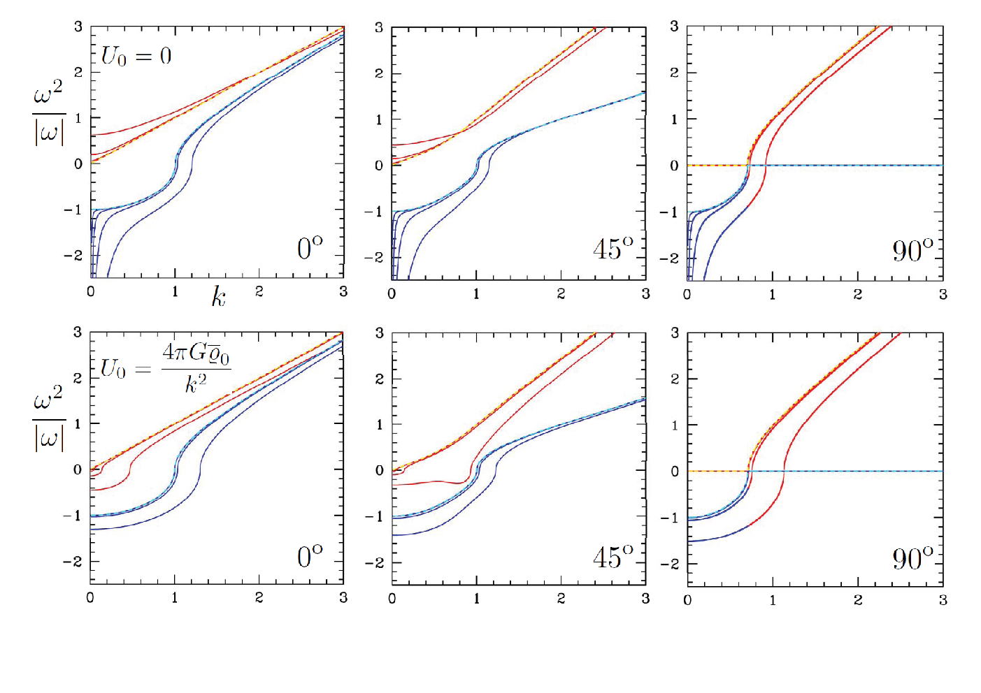
Behaviors of the 1PN solutions compared with the Newtonian ones are presented in Figures 2 and 3 for U0=0U_{0}=0 and 4​π​G​ϱ¯0/k24\pi G\overline{\varrho}_{0}/k^{2}, respectively, for a rather strong relativistic situation with R≡cs2/c2=0.01R\equiv c_{s}^{2}/c^{2}=0.01. Dependence on RR is presented in Figure 4. As our analysis is valid to 1PN order the solutions in Equation (80) can be Taylor expanded to 1PN order. In the Figures we plot these expanded solutions.

Refer to caption
Figure 2.— Behaviors of two 1PN solutions (solid lines) in Equation (80) for U0=0U_{0}=0 compared with the Newtonian ones (dashed lines) in Equation (56); the upper (plus) and lower (minus) signs correspond to red and blue lines for 1PN, and magenta and cyan lines for for Newtonian, respectively. We set Π0=0=p0\Pi_{0}=0=p_{0}, and consider R≡cs2/c2=0.01R\equiv c_{s}^{2}/c^{2}=0.01, s=0.5s=0.5, 11 and 22, and ψ=0o\psi=0^{\rm o}, 45o45^{\rm o} and 90o90^{\rm o}. Units are the same as in Figure 1.
Refer to caption
Figure 3.— The same as Figure 2 for U0=4​π​G​ϱ¯0/k2U_{0}=4\pi G\overline{\varrho}_{0}/k^{2}.
Refer to caption
Figure 4.— Dependence on R≡cs2/c2R\equiv c_{s}^{2}/c^{2} for R=0.1R=0.1, 0.010.01, 0.0010.001 and 0.00010.0001; the 1PN results (solid red and blue lines) approach the Newtonian ones (dashed yellow and cyan lines) as RR decreases. The upper and lower figures correxpond to U0=0U_{0}=0 and U0=4​π​G​ϱ¯0/k2U_{0}=4\pi G\overline{\varrho}_{0}/k^{2}, respectively. We consider ψ=0o\psi=0^{\rm o}, 45o45^{\rm o} and 90o90^{\rm o} for s≡cA2/cs2=1s\equiv c_{A}^{2}/c_{s}^{2}=1 and Π0=0=p0\Pi_{0}=0=p_{0}.

Notice that, in Figure 2 for vanishing U0U_{0}, the 1PN correction terms cause ω2\omega^{2} to diverge for small kk (large-scale) limit. For k→0k\rightarrow 0, including U0U_{0}, we have

ω24​π​G​ϱ¯0​[1+1c2​(Π0+p0ϱ¯0)]\displaystyle{\omega^{2}\over 4\pi G\overline{\varrho}_{0}}\left[1+{1\over c^{2}}\left(\Pi_{0}+{p_{0}\over\overline{\varrho}_{0}}\right)\right]
=0,−1−2​4​π​G​ϱ¯0k2​c2+2​U0c2.\displaystyle\qquad=0,\quad-1-2{4\pi G\overline{\varrho}_{0}\over k^{2}c^{2}}+2{U_{0}\over c^{2}}. (81)

Thus, for vanishing U0U_{0}, for small enough kk, the PN correction terms cause the system more unstable and the exponent i​ωi\omega diverges. The diverging instability due to the 1PN correction may imply breakdown of the 1PN approximation; this was noticed by Nazari et al (2017) in the absence of magnetic field. By demanding the 1PN correction terms to be smaller than the 0PN order, we have

k2>2​4​π​G​ϱ¯0c2.\displaystyle k^{2}>2{4\pi G\overline{\varrho}_{0}\over c^{2}}. (82)

In terms of wavelength, λ=2​π/k\lambda=2\pi/k, the 1PN approximation demands

λ<c​π2​G​ϱ¯0∼c​tg,\displaystyle\lambda<c\sqrt{\pi\over 2G\overline{\varrho}_{0}}\sim ct_{g}, (83)

where tg≡1/G​ϱ¯0t_{g}\equiv 1/\sqrt{G\overline{\varrho}_{0}} is the gravitational timescale. The diverging instability for λ\lambda greater than c​tgct_{g} (the light propagation distance during gravitational timescale) is consistent with the eventual instability of the background system [known and studied in cosmology by Friedmann (1922, 1924) and Bonnor (1957)] which we have ignored by taking the Minkowski background. In a conservative stance, however, this simply implies the limit of the 1PN approximation.

On the other hand, in Figure 3 for U0=4​π​G​ϱ¯0/k2U_{0}=4\pi G\overline{\varrho}_{0}/k^{2}, the 1PN correction terms in Equation (81) disappear. In the k→0k\rightarrow 0 limit, to the next leading order we have

ω24​π​G​ϱ¯0​[1+1c2​(Π0+p0ϱ¯0)]=−2c2​cA2​cos2⁡ψ,\displaystyle{\omega^{2}\over 4\pi G\overline{\varrho}_{0}}\left[1+{1\over c^{2}}\left(\Pi_{0}+{p_{0}\over\overline{\varrho}_{0}}\right)\right]=-{2\over c^{2}}c_{A}^{2}\cos^{2}{\psi},
−1−1c2​(7​cs2+6​cA2​sin2⁡ψ).\displaystyle\qquad-1-{1\over c^{2}}\left(7c_{s}^{2}+6c_{A}^{2}\sin^{2}{\psi}\right). (84)

For 𝐤|𝐁0{\bf k}\parallel{\bf B}_{0} (ψ=0o\psi=0^{\rm o}), we have

ω2k2​[1+1c2​(Π0+p0ϱ¯0)]\displaystyle{\omega^{2}\over k^{2}}\left[1+{1\over c^{2}}\left(\Pi_{0}+{p_{0}\over\overline{\varrho}_{0}}\right)\right]
=cs2−4​π​G​ϱ¯0k2+1c2​(cs2−4​π​G​ϱ¯0k2)​𝒜−cA2​ℬcs2−cA2−4​π​G​ϱ¯0k2,\displaystyle\qquad=c_{s}^{2}-{4\pi G\overline{\varrho}_{0}\over k^{2}}+{1\over c^{2}}{\left(c_{s}^{2}-{4\pi G\overline{\varrho}_{0}\over k^{2}}\right){\cal A}-c_{A}^{2}{\cal B}\over c_{s}^{2}-c_{A}^{2}-{4\pi G\overline{\varrho}_{0}\over k^{2}}},
cA2+1c2​cA2​(−𝒜+ℬ)cs2−cA2−4​π​G​ϱ¯0k2.\displaystyle\qquad c_{A}^{2}+{1\over c^{2}}{c_{A}^{2}\left(-{\cal A}+{\cal B}\right)\over c_{s}^{2}-c_{A}^{2}-{4\pi G\overline{\varrho}_{0}\over k^{2}}}. (85)

One mode is unstable and the critical (Jeans) wavenumber becomes

kJ2=4​π​G​ϱ¯0cs2​[1+1c2​(2​Π0+2​p0ϱ¯0+5​cs2+2​U0)].\displaystyle k_{J}^{2}={4\pi G\overline{\varrho}_{0}\over c_{s}^{2}}\left[1+{1\over c^{2}}\left(2\Pi_{0}+2{p_{0}\over\overline{\varrho}_{0}}+5c_{s}^{2}+2U_{0}\right)\right]. (86)

This coincides exactly with the Jeans wavenumber in the absence of the magnetic field, see Equation (91); thus, the criterion does not depend on the magnetic field as emphasized by Chandrasekhar & Fermi (1953), now even to 1PN order, see below Equation (58). In the absence of gravity, we have

ω2k2​[1+1c2​(Π0+p0ϱ¯0)]=cs2,cA2​(1−cA2c2).\displaystyle{\omega^{2}\over k^{2}}\left[1+{1\over c^{2}}\left(\Pi_{0}+{p_{0}\over\overline{\varrho}_{0}}\right)\right]=c_{s}^{2},\quad c_{A}^{2}\left(1-{c_{A}^{2}\over c^{2}}\right). (87)

For 𝐤⟂𝐁0{\bf k}\perp{\bf B}_{0} (ψ=90o\psi=90^{\rm o}), we have

ω2k2=cs2​[1−1c2​(Π0+p0ϱ¯0+cA2+3​4​π​G​ϱ¯0k2+4​U0)]+cA2​[1−1c2​(Π0+p0ϱ¯0+cA2+4​π​G​ϱ¯0k2+6​U0)]\displaystyle{\omega^{2}\over k^{2}}=c_{s}^{2}\left[1-{1\over c^{2}}\left(\Pi_{0}+{p_{0}\over\overline{\varrho}_{0}}+c_{A}^{2}+3{4\pi G\overline{\varrho}_{0}\over k^{2}}+4U_{0}\right)\right]+c_{A}^{2}\left[1-{1\over c^{2}}\left(\Pi_{0}+{p_{0}\over\overline{\varrho}_{0}}+c_{A}^{2}+{4\pi G\overline{\varrho}_{0}\over k^{2}}+6U_{0}\right)\right]
−4​π​G​ϱ¯0k2​[1+1c2​(Π0+p0ϱ¯0−cA2+2​4​π​G​ϱ¯0k2−2​U0)],0.\displaystyle\qquad-{4\pi G\overline{\varrho}_{0}\over k^{2}}\left[1+{1\over c^{2}}\left(\Pi_{0}+{p_{0}\over\overline{\varrho}_{0}}-c_{A}^{2}+2{4\pi G\overline{\varrho}_{0}\over k^{2}}-2U_{0}\right)\right],\quad 0. (88)

The critical wavenumber of the unstable mode becomes

kB2=4​π​G​ϱ¯0cs2+cA2​[1+1c2​(2​Π0+2​p0ϱ¯0+3​cA2+5​cs2+2​U0​cs2+2​cA2cs2+cA2)].\displaystyle k_{B}^{2}={4\pi G\overline{\varrho}_{0}\over c_{s}^{2}+c_{A}^{2}}\left[1+{1\over c^{2}}\left(2\Pi_{0}+2{p_{0}\over\overline{\varrho}_{0}}+3c_{A}^{2}+5c_{s}^{2}+2U_{0}{c_{s}^{2}+2c_{A}^{2}\over c_{s}^{2}+c_{A}^{2}}\right)\right]. (89)

Now the choice for U0U_{0} can be made. We can either ignore the U0U_{0} terms (Jeans’ choice), or use Equation (62) to 0PN order, thus U0=4​π​G​ϱ¯0/k2U_{0}=4\pi G\overline{\varrho}_{0}/k^{2}. In the latter choice we have U0=cs2U_{0}=c_{s}^{2} in Equation (86) and U0=cs2+cA2U_{0}=c_{s}^{2}+c_{A}^{2} in Equation (89).

Equations (86) and (89) show that the 1PN corrections of the internal energy, pressure, sound velocity and the Alfvén velocity cause to decrease of critical (Jeans) wavelength, λ=2​π/k\lambda=2\pi/k, thus reduce the Jeans mass, M≡(π/6)​ϱ¯​λ3M\equiv(\pi/6)\overline{\varrho}\lambda^{3}, Figures 2-4 more generally show that for all ψ\psi values the 1PN effects tend to increase the critical wavenumber (thus lower the critical wavelength) and make more negative ω2\omega^{2} (thus making system more unstable). Therefore, we conclude that, to 1PN order, all relativistic corrections tend to destabilize the system.

V.1. Limiting cases

Here, we compare our results with previous studies.

(i) To 0PN order we recover Equation (55); Equation (169) in Chandrasekhar & Fermi (1953).

(ii) Ignoring gravity, thus setting U0≡0≡4​π​G​ϱ¯0U_{0}\equiv 0\equiv 4\pi G\overline{\varrho}_{0}, we recover the 1PN MHD waves in Section 7 of Hwang & Noh (2020).

(iii) For vanishing magnetic field with 𝐁=0{\bf B}=0, thus setting 𝐧=0=cA2{\bf n}=0=c_{A}^{2}, from Equation (72) we have

{ω2k2​[1+1c2​(Π0+p0ϱ¯0+3​4​π​G​ϱ¯0k2+4​U0)]−cs2+4​π​G​ϱ¯0k2​[1+1c2​(2​Π0+2​p0ϱ¯0+5​4​π​G​ϱ¯0k2+2​U0)]}​𝐤⋅𝐯=0.\displaystyle\bigg\{{\omega^{2}\over k^{2}}\left[1+{1\over c^{2}}\left(\Pi_{0}+{p_{0}\over\overline{\varrho}_{0}}+3{4\pi G\overline{\varrho}_{0}\over k^{2}}+4U_{0}\right)\right]-c_{s}^{2}+{4\pi G\overline{\varrho}_{0}\over k^{2}}\left[1+{1\over c^{2}}\left(2\Pi_{0}+2{p_{0}\over\overline{\varrho}_{0}}+5{4\pi G\overline{\varrho}_{0}\over k^{2}}+2U_{0}\right)\right]\bigg\}{\bf k}\cdot{\bf v}=0. (90)

By setting ω=0\omega=0 we have k=kJk=k_{J} with

kJ2=4​π​G​ϱ¯0cs2​[1+1c2​(2​Π0+2​p0ϱ¯0+5​cs2+2​U0)].\displaystyle k_{J}^{2}={4\pi G\overline{\varrho}_{0}\over c_{s}^{2}}\left[1+{1\over c^{2}}\left(2\Pi_{0}+2{p_{0}\over\overline{\varrho}_{0}}+5c_{s}^{2}+2U_{0}\right)\right]. (91)

This also follows from Equation (80). By choosing U0=4​π​G​ϱ¯0/k2U_{0}=4\pi G\overline{\varrho}_{0}/k^{2}, we have U0=cs2U_{0}=c_{s}^{2} in Equation (91). Therefore, the PN corrections of the internal energy, pressure and sound velocity lower the critical (Jeans) wavelength. Thus, as generally shown even in the presence of magnetic field, all relativistic corrections tend to destabilize the system.

Equation (91), setting U0=0U_{0}=0, differs from the result in Equation (56) of Nazari et al (2017) in the coefficient of cs2c_{s}^{2}. In our approach of separating the 0PN and 1PN orders clearly, the difference is caused by mixed decomposition of the 0PN and 1PN orders, for example, in Equations (3) and (5) of Nazari et al (2017); by moving the 1PN order terms in Equation (3) properly to Equation (5) one can recover our result.

In Nazari et al (2017)’s approach, however, the 0PN and 1PN orders are not separated. Compared to our cs2c_{s}^{2} based on p=p⁡(ϱ¯)p=p(\overline{\varrho}), thus cs2≡δ​p/δ​ϱ¯c_{s}^{2}\equiv\delta p/\delta\overline{\varrho}, their cs2c_{s}^{2} is based on p=p⁡(ϱ∗)p=p(\varrho^{*}), thus cs2≡δ​p/δ​ϱ∗c_{s}^{2}\equiv\delta p/\delta\varrho^{*}; ϱ∗\varrho^{*} is the conserved density to 1PN order introduced by Chandrasekhar (1965)

ϱ∗≡ϱ¯​[1+1c2​(12​v2+3​U)].\displaystyle\varrho^{*}\equiv\overline{\varrho}\left[1+{1\over c^{2}}\left({1\over 2}v^{2}+3U\right)\right]. (92)

With this Equation (6) can be written as

∂∂t​ϱ∗+∇⋅(ϱ∗​𝐯¯)=0.\displaystyle{\partial\over\partial t}\varrho^{*}+\nabla\cdot\left(\varrho^{*}\overline{\bf v}\right)=0. (93)

Notice that ϱ∗\varrho^{*} is already 1PN order, and the same for cs2c_{s}^{2} defined based on ϱ∗\varrho^{*}. Using this difference in the definition of cs2c_{s}^{2} we can also recover the 55 factor in the coefficient of our cs2c_{s}^{2}. In this way the standard Jeans wavenumber in Equations (26) and (35) of Nazari et al (2017) already contains the 1PN order; similarly all results in that paper are presented with the 0PN and 1PN orders not clearly separated. Qualitatively, however, as the coefficient of cs2c_{s}^{2} is changed from 22 to 55 without the sign change, the reducing effect on the Jeans wavelength due to the PN sound velocity is not changed. (We thank Professor Mahmood Roshan and Dr. Elham Nazari for communications concerning their work.)

VI. Stability of SR MHD

We consider the same background medium with an aligned magnetic field. To the background order, we have a solution with

ϱ¯0=constant,Π0=constant,p0=constant,\displaystyle\overline{\varrho}_{0}={\rm constant},\quad\Pi_{0}={\rm constant},\quad p_{0}={\rm constant},
𝐁0=B0​𝐧=constant,𝐯0=0,∇Φ0=0,\displaystyle{\bf B}_{0}=B_{0}{\bf n}={\rm constant},\quad{\bf v}_{0}=0,\quad\nabla\Phi_{0}=0, (94)

but we have

Δ​Φ0=4​π​G​(ϱ0+3​p0c2+1c2​14​π​B02).\displaystyle\Delta\Phi_{0}=4\pi G\left(\varrho_{0}+{3p_{0}\over c^{2}}+{1\over c^{2}}{1\over 4\pi}B_{0}^{2}\right). (95)

Thus, the inconsistency concerning Φ0\Phi_{0} remains, but as in the Newtonian case Φ0\Phi_{0} does not appear in the perturbation analysis, and we can ignore Equation (95), see a paragraph below Equation (40).

To the linear order, Equations (III)-(31) give

∂∂t​(DEmiBi)+∇j(D​vjmj​c2mi​jvj​Bi−vi​Bj)=(00−ϱ¯Φ,i0),\displaystyle{\partial\over\partial t}\left(\begin{array}[]{c}D\\ E\\ m^{i}\\ B^{i}\end{array}\right)+\nabla_{j}\left(\begin{array}[]{c}Dv^{j}\\ m^{j}c^{2}\\ m^{ij}\\ v^{j}B^{i}-v^{i}B^{j}\end{array}\right)=\left(\begin{array}[]{c}0\\ 0\\ -\overline{\varrho}\Phi^{,i}\\ 0\end{array}\right),
Bi,i=0,\displaystyle B^{i}_{\;\;,i}=0, (109)
Δ​Φ=4​π​G​(ϱ+3​pc2+1c2​14​π​B2),\displaystyle\Delta\Phi=4\pi G\left(\varrho+{3p\over c^{2}}+{1\over c^{2}}{1\over 4\pi}B^{2}\right), (110)

with

D=ϱ¯,E/c2=ϱ+1c2​18​π​B2,\displaystyle D=\overline{\varrho},\quad E/c^{2}=\varrho+{1\over c^{2}}{1\over 8\pi}B^{2},
mi=(ϱ+pc2)​vi+1c2​14​π​(B2​vi−Bi​Bj​vj),\displaystyle m^{i}=\left(\varrho+{p\over c^{2}}\right)v^{i}+{1\over c^{2}}{1\over 4\pi}\left(B^{2}v^{i}-B^{i}B^{j}v_{j}\right),
mi​j=p​δi​j+14​π​(12​B2​δi​j−Bi​Bj).\displaystyle m^{ij}=p\delta^{ij}+{1\over 4\pi}\left({1\over 2}B^{2}\delta^{ij}-B^{i}B^{j}\right). (111)

Equations (32) and (34) are not needed.

Equations (VI)-(110) can be arranged to give

δ˙=−∇⋅𝐯,\displaystyle\dot{\delta}=-\nabla\cdot{\bf v}, (112)
δΠ˙=−p0ϱ¯0∇⋅𝐯,\displaystyle\delta\dot{\Pi}=-{p_{0}\over\overline{\varrho}_{0}}\nabla\cdot{\bf v}, (113)
[1+1c2​(Π0+p0ϱ¯0+cA2)]​𝐯˙−1c2​cA2​𝐧𝐧⋅𝐯˙\displaystyle\left[1+{1\over c^{2}}\left(\Pi_{0}+{p_{0}\over\overline{\varrho}_{0}}+c_{A}^{2}\right)\right]\dot{\bf v}-{1\over c^{2}}c_{A}^{2}{\bf n}{\bf n}\cdot\dot{\bf v}
+cs2∇δ+∇δΦ=cA2[𝐧⋅∇𝐛−∇(𝐧⋅𝐛)],\displaystyle\qquad+c_{s}^{2}\nabla\delta+\nabla\delta\Phi=c_{A}^{2}\left[{\bf n}\cdot\nabla{\bf b}-\nabla\left({\bf n}\cdot{\bf b}\right)\right], (114)
Δ​δ​Φ=4​π​G​ϱ¯0​[δ+1c2​(Π0​δ+δ​Π+3​cs2​δ+2​cA2​𝐧⋅𝐛)],\displaystyle\Delta\delta\Phi=4\pi G\overline{\varrho}_{0}\left[\delta+{1\over c^{2}}\left(\Pi_{0}\delta+\delta\Pi+3c_{s}^{2}\delta+2c_{A}^{2}{\bf n}\cdot{\bf b}\right)\right],
(115)
𝐛˙=𝐧⋅∇𝐯−𝐧∇⋅𝐯,\displaystyle\dot{\bf b}={\bf n}\cdot\nabla{\bf v}-{\bf n}\nabla\cdot{\bf v}, (116)
∇⋅𝐛=0.\displaystyle\nabla\cdot{\bf b}=0. (117)

These can be compared with Equations (64)-(70) in the PN case. As mentioned in a paragraph below Equation (34), to be consistent we need δ​Φ\delta\Phi only to the Newtonian order in Equation (115); thus, Δ​δ​Φ=4​π​G​ϱ¯0​δ\Delta\delta\Phi=4\pi G\overline{\varrho}_{0}\delta; in the same spirit we ignore gravity terms combined with relativistic (PN) order, like 4​π​G​ϱ¯0/(k2​c2)4\pi G\overline{\varrho}_{0}/(k^{2}c^{2}). Thus, we do not need Equation (113). Compared with Newtonian Equations (43)-(47) differences occur only in the coefficients of 𝐯˙\dot{\bf v} terms in Equation (114).

Expanding in plane waves we can derive

{[1+1c2​(Π0+p0ϱ¯0+cA2)]​ω2−cA2​(𝐧⋅𝐤)2}​𝐯+[(4​π​G​ϱ¯0k2−cs2−cA2)​𝐤+cA2​𝐧𝐧⋅𝐤]​𝐤⋅𝐯\displaystyle\left\{\left[1+{1\over c^{2}}\left(\Pi_{0}+{p_{0}\over\overline{\varrho}_{0}}+c_{A}^{2}\right)\right]\omega^{2}-c_{A}^{2}\left({\bf n}\cdot{\bf k}\right)^{2}\right\}{\bf v}+\left[\left({4\pi G\overline{\varrho}_{0}\over k^{2}}-c_{s}^{2}-c_{A}^{2}\right){\bf k}+c_{A}^{2}{\bf n}{\bf n}\cdot{\bf k}\right]{\bf k}\cdot{\bf v}
+cA2(𝐤𝐤⋅𝐧−1c2ω2𝐧)𝐧⋅𝐯=0.\displaystyle\qquad+c_{A}^{2}\left({\bf k}{\bf k}\cdot{\bf n}-{1\over c^{2}}\omega^{2}{\bf n}\right){\bf n}\cdot{\bf v}=0. (118)

By taking a coordinate in Equation (49), Equation (118) gives

{[1+1c2​(Π0+p0ϱ¯0+cA2​sin2⁡ψ)]​ω2−k2​(cs2+cA2​sin2⁡ψ)+4​π​G​ϱ¯0}​vx+(k2−1c2​ω2)​cA2​sin⁡ψ​cos⁡ψ​vy=0,\displaystyle\bigg\{\left[1+{1\over c^{2}}\left(\Pi_{0}+{p_{0}\over\overline{\varrho}_{0}}+c_{A}^{2}\sin^{2}{\psi}\right)\right]\omega^{2}-k^{2}\left(c_{s}^{2}+c_{A}^{2}\sin^{2}{\psi}\right)+4\pi G\overline{\varrho}_{0}\bigg\}v_{x}+\left(k^{2}-{1\over c^{2}}\omega^{2}\right)c_{A}^{2}\sin{\psi}\cos{\psi}v_{y}=0, (119)
(k2−1c2​ω2)​cA2​sin⁡ψ​cos⁡ψ​vx+{[1+1c2​(Π0+p0ϱ¯0+cA2​cos2⁡ψ)]​ω2−cA2​k2​cos2⁡ψ}​vy=0,\displaystyle\left(k^{2}-{1\over c^{2}}\omega^{2}\right)c_{A}^{2}\sin{\psi}\cos{\psi}v_{x}+\bigg\{\left[1+{1\over c^{2}}\left(\Pi_{0}+{p_{0}\over\overline{\varrho}_{0}}+c_{A}^{2}\cos^{2}{\psi}\right)\right]\omega^{2}-c_{A}^{2}k^{2}\cos^{2}{\psi}\bigg\}v_{y}=0, (120)
{[1+1c2​(Π0+p0ϱ¯0+cA2)]​ω2−cA2​k2​cos2⁡ψ}​vz=0.\displaystyle\left\{\left[1+{1\over c^{2}}\left(\Pi_{0}+{p_{0}\over\overline{\varrho}_{0}}+c_{A}^{2}\right)\right]\omega^{2}-c_{A}^{2}k^{2}\cos^{2}{\psi}\right\}v_{z}=0. (121)

For vz≠0v_{z}\neq 0 (𝐯{\bf v} perpendicular to 𝐁0{\bf B}_{0}-𝐤{\bf k} plane), Equation (121) gives

ω2k2=cA2​cos2⁡ψ1+1c2​(Π0+p0ϱ¯0+cA2).\displaystyle{\omega^{2}\over k^{2}}={c_{A}^{2}\cos^{2}{\psi}\over 1+{1\over c^{2}}\left(\Pi_{0}+{p_{0}\over\overline{\varrho}_{0}}+c_{A}^{2}\right)}. (122)

For non-vanishing vxv_{x} and vyv_{y} (𝐯{\bf v} in 𝐁𝟎{\bf B_{0}}-𝐤{\bf k} plane), from Equations (119) and (120) we have

ω4k4​[1+1c2​(Π0+p0ϱ¯0)]​[1+1c2​(Π0+p0ϱ¯0+cA2)]\displaystyle{\omega^{4}\over k^{4}}\left[1+{1\over c^{2}}\left(\Pi_{0}+{p_{0}\over\overline{\varrho}_{0}}\right)\right]\left[1+{1\over c^{2}}\left(\Pi_{0}+{p_{0}\over\overline{\varrho}_{0}}+c_{A}^{2}\right)\right]
−ω2k2{(cs2+cA2)[1+1c2(Π0+p0ϱ¯0)]\displaystyle\qquad-{\omega^{2}\over k^{2}}\bigg\{\left(c_{s}^{2}+c_{A}^{2}\right)\left[1+{1\over c^{2}}\left(\Pi_{0}+{p_{0}\over\overline{\varrho}_{0}}\right)\right]
+1c2cs2cA2cos2ψ−4​π​G​ϱ¯0k2}\displaystyle\qquad+{1\over c^{2}}c_{s}^{2}c_{A}^{2}\cos^{2}{\psi}-{4\pi G\overline{\varrho}_{0}\over k^{2}}\bigg\}
+cA2​cos2⁡ψ⁡(cs2−4​π​G​ϱ¯0k2)=0,\displaystyle\qquad+c_{A}^{2}\cos^{2}{\psi}\left(c_{s}^{2}-{4\pi G\overline{\varrho}_{0}\over k^{2}}\right)=0, (123)

with two solutions for ω2/k2\omega^{2}/k^{2}.

For 𝐤|𝐁0{\bf k}\parallel{\bf B}_{0} (ψ=0o\psi=0^{\rm o}), we have

ω2k2=cs21+1c2​(Π0+p0ϱ¯0)−4​π​G​ϱ¯0k2,\displaystyle{\omega^{2}\over k^{2}}={c_{s}^{2}\over 1+{1\over c^{2}}\left(\Pi_{0}+{p_{0}\over\overline{\varrho}_{0}}\right)}-{4\pi G\overline{\varrho}_{0}\over k^{2}},\quad
cA21+1c2​(Π0+p0ϱ¯0+cA2).\displaystyle\qquad{c_{A}^{2}\over 1+{1\over c^{2}}\left(\Pi_{0}+{p_{0}\over\overline{\varrho}_{0}}+c_{A}^{2}\right)}. (124)

One mode is unstable and the critical (Jeans) wavenumber becomes

kJ2=4​π​G​ϱ¯0cs2,\displaystyle k_{J}^{2}={4\pi G\overline{\varrho}_{0}\over c_{s}^{2}}, (125)

as the gravity part is valid only to the Newtonian order.

For 𝐤⟂𝐁0{\bf k}\perp{\bf B}_{0} (ψ=90o\psi=90^{\rm o}), we have

ω2k2=cs2+cA21+1c2​(Π0+p0ϱ¯0+cA2)−4​π​G​ϱ¯0k2,0.\displaystyle{\omega^{2}\over k^{2}}={c_{s}^{2}+c_{A}^{2}\over 1+{1\over c^{2}}\left(\Pi_{0}+{p_{0}\over\overline{\varrho}_{0}}+c_{A}^{2}\right)}-{4\pi G\overline{\varrho}_{0}\over k^{2}},\quad 0. (126)

The critical wavenumber of the unstable mode similarly becomes

kB2=4​π​G​ϱ¯0cs2+cA2.\displaystyle k_{B}^{2}={4\pi G\overline{\varrho}_{0}\over c_{s}^{2}+c_{A}^{2}}. (127)

As mentioned, as we consider the gravity the stability analysis is consistent only to the Newtonian order, thus Equations (125) and (127) are the same as in the Newtonian MHD. Whereas, considering gravity only to the Newtonian order, the wave solutions in Equations (122), (124) and (126), and the two general solutions of Equation (123) for general ψ\psi are valid for the fully SR MHD. In the absence of gravity, the wave speeds in Equations (122), (124) and (126) include the 1PN results in Equations (76), (87) and (88) as the 1PN limit.

VII. Summary

Sections II and III are summaries of two formulations of relativistic MHD: MHD valid to 1PN approximation and the SR MHD with weak gravity. The equations of PN MHD are presented without taking the slicing condition, whereas the equations of SR MHD with weak gravity are valid in the maximal slicing which corresponds to the harmonic gauge in the PN formulation. Section IV is the MHD instability of the the homogeneous medium with an aligned magnetic field in Newtonian (0PN) limit, largely overlapping with previous studies in Chandrasekhar & Fermi (1954) and Chandrasekhar (1954, 1961). Here, we clarify some unclear remarks made in the previous works concerning effects of magnetic field on the gravitational instability, see below our Equations (58) and (60). We also address the inconsistency issue related to the Poisson’s equation to the homogeneous background medium, see paragraphs below Equation (40) and below Equation (71).

Section V presents our main analysis of the 1PN gravito-magnetic instability of the same medium. We show that the post-Newtonian corrections of the internal energy (Π0\Pi_{0}), pressure (p0p_{0}), sound velocity (csc_{s}) and the Alfvén velocity (cAc_{A}) consistently lower the Jeans wavelength and the Jeans mass, see Equations (86) and (89), and tend to destabilize the system, see Figures 2-4. We note that we have not fixed the temporal gauge condition for the analysis, thus the results are valid independently of the gauge condition and are naturally gauge invariant, see Section 6.3 in Hwang & Noh (2020).

Section VI presents another main analysis of the waves and instability of the SR MHD with weak gravity. The MHD waves of the SR MHD are presented in Equations (122)-(124) and (126). When we consider the gravity however, the analysis is consistent to Newtonian order only, and the critical wavenumbers in Equations (125) and (127) are the same as in the Newtonian MHD.

VIII. Discussion

Stability analysis of an infinite homogeneous medium is a textbook exercise in the Newtonian case; gravitational instability in the presence of aligned magnetic field is rarely presented though (Chandrasekhar 1961). The exponential instability for an imaginary ω\omega indicates no lack-of-time problem in the gravitational collapse in a static medium: i.e., the over-dense region larger than Jeans scale may collapse immediately. This may have a negative side though that we can hardly find astrophysical situations where the conditions (static homogeneous medium, let aside the infinity condition) are met in the interstellar space. Interstellar matter and molecular clouds, in fact, are known to be in the state of (compressible) turbulence (Elmegreen & Scalo 2004).

Although the infinite static homogeneous background medium has the internal inconsistency (which remains even in the relativistic situation as we have shown in this work) the Jeans stability criterion survives in a consistent relativistic analysis made in infinite homogeneous, but dynamic, background medium (Lifshitz 1946); in the static limit we recover the Jeans result! In a power-law expanding medium (like in the matter dominated era) the growth rate is suppressed from exponential to a decelerating power-law; this was originally recognized as too slow to serve for galaxy or star formation by Lifshitz (1946). Nowadays, our observable universe provides a prime example with highly successful gravitational instability as the main driving engine of the large-scale structure with a long duration (due to slow growth rate) from its generation in the early universe till even today.

Lifshitz’s stability analysis, however, is made in the absence of magnetic field. In the presence of aligned magnetic field, the proper relativistic analysis demands other than the Friedmann cosmology with the anisotropic cosmological principle (Thorne 1967). Current success in cosmology does not encourage such a study, and which part of our study could survive the consistent analysis (in the static limit) is currently unknown.

As the static homogeneous medium is not realistic (i.e, cannot or rarely be found) in known astrophysical environments, an additional aligned magnetic field is also apparently not realistic. Our motivation for choosing the situation is to extend the textbook analysis of the gravito-magnetic instability known in Newtonian MHD to a couple of relativistic situations. We have shown that the inconsistency noticed by Jeans is due to the static nature of the background medium. The relativistic analysis can cure the inconsistency by demanding dynamic background medium (Lifshitz 1946; Hwang, Noh & Puetzfeld 2008).

More realistic astrophysical situations where relativistic MHD is needed can be found in accretion discs, magnetospheres, the plasma winds and astrophysical jets near compact astrophysical objects (like neutron stars and black holes), and active galactic nuclei. Such situations may require the spherical, cylindrical or disc geometries (Thorne, Price & Macdonald 1986; Beskin 2010). Stability analysis in these weakly relativistic situations using our two new relativistic MHD formulations summarized in Sections II and III will be interesting. Being fully nonlinear, these two relativistic MHD formulation may be convenient to numerically handle the weakly relativistic (1PN approximation) or weak gravity situations.

Acknowledgments

We wishes to thank the referee for constructive comments. J.H. was supported by Basic Science Research Program through the National Research Foundation (NRF) of Korea funded by the Ministry of Science, ICT and future Planning (No. 2018R1A6A1A06024970 and NRF-2019R1A2C1003031). H.N. was supported by National Research Foundation of Korea funded by the Korean Government (No. 2018R1A2B6002466).

References

  • (1) Beskin, V. S. 2010, MHD Flows in Compact Astrophysical Objects, (Springer, Berlin)
  • (2) Bonnor, W. B. 1957, Mon. Not. Roy. Astron. Soc. 117, 104
  • (3) Chandrasekhar, S. 1954, ApJ, 119, 7
  • (4) Chandrasekhar, S. 1961, Hydrodynamic and Hydromagnetic Stability (Oxford University Press)
  • (5) Chandrasekhar, S. 1965, ApJ, 142, 1488
  • (6) Chandrasekhar, S., & Fermi, E. 1953, ApJ, 118, 116
  • (7) Chandrasekhar, S., & Nutku, Y. 1969, ApJ, 158, 55
  • (8) Friedmann, A. A. 1922, Zeit. für Physik 10, 377; English. transl. 1999, in Gen. Rel. Grav. 31, 1991
  • (9) Friedmann, A. A. 1924, Zeit. für Physik 21, 326; English. transl. 1999, in Gen. Rel. Grav. 31, 2001
  • (10) Greenberg, P. J. 1971, ApJ, 164, 589
  • (11) Hwang, J., & Noh, H. 2013, JCAP, 04, 035
  • (12) Hwang, J., & Noh, H. 2020, ApJ, 899, 59
  • (13) Hwang, J., Noh, H., & Puetzfeld, D. 2008, JCAP, 03, 010
  • (14) Jeans, J. H. 1902, Phil. Trans. R. Soc. London A., 199, 1
  • (15) Lifshitz, E. M. 1946, J. Phys. (USSR) 10, 116; English transl. reprinted in 2017, Gen. Rel. Grav. 49, 18
  • (16) Nazari, E., Kazemi, A., Roshan, M., & Abbassi, S. 2017, ApJ, 839, 75
  • (17) Nazari, E., & Roshan, M. 2018, ApJ, 868, 98
  • (18) Noh, H., Hwang, J., & Bucher, M. 2019, ApJ, 877, 124
  • (19) Pacholczyk, A. G., & Stodółkiewicz, J. S. 1960, Acta Astronomica, 10, 1
  • (20) Poisson, E., & Will, C. M. 2014, Gravity: Newtonian, Post-Newtonian, Relativistic (Cambridge Univ. Press)
  • (21) Elmegreen, B. G., & Scalo, J. 2004, Ann. Rev. Astron. Astrophys., 42, 211
  • (22) Shu, F. H. 1992, The Physics of Astrophysics vol II Gas Dynamics (University Science Books)
  • (23) Strittmatter, P. A. 1966, Mon. Not. Roy. Astron. Soc. 131, 491
  • (24) Thorne, K. 1967, ApJ, 148, 51
  • (25) Thorne, K. S., Price, R. H., & MacDonald, D. A. 1986, Black Holes: The Membrane Paradigm (Yale University Press, London)