跳到论文正文
W Papers独立论文阅读器 arXiv:2010.01332 论文正文 计算阅读时间 · 0%
引用这篇论文根据当前论文元数据生成,正式投稿前建议核对。


License: arXiv.org perpetual non-exclusive license
arXiv:2010.01332v2 [cond-mat.mes-hall] 01 Oct 2021

Inter- and intra-band Coulomb interactions between holes in silicon nanostructures

Andrea Secchi Email: andrea.secchi@nano.cnr.it Affiliation: Centro S3, CNR-Istituto di Nanoscienze, via G. Campi 213/A, I-41125 Modena, Italy    Laura Bellentani Affiliation: Centro S3, CNR-Istituto di Nanoscienze, via G. Campi 213/A, I-41125 Modena, Italy    Andrea Bertoni Affiliation: Centro S3, CNR-Istituto di Nanoscienze, via G. Campi 213/A, I-41125 Modena, Italy    Filippo Troiani Affiliation: Centro S3, CNR-Istituto di Nanoscienze, via G. Campi 213/A, I-41125 Modena, Italy
August 11, 2026
Abstract

We present a full derivation of the interaction Hamiltonian for holes in silicon within the six–band envelope-function scheme, which appropriately describes the valence band close to the 𝚪\bm{\Gamma} point. The full structure of the single-hole eigenstates is taken into account, including the Bloch part. The scattering processes caused by the Coulomb interaction are shown to be both intraband and interband, the latter being mostly short-ranged. In the asymptotic long-range limit, the effective potential tends to the screened Coulomb potential, and becomes purely intraband, as assumed in previous models. We apply our model to compute the excitation spectra of two interacting holes in prototypical silicon quantum dots, taking into account different dielectric environments. It is shown that, in the highly screened regime, short-range interactions (both intra- and inter-band) can be very relevant, while they lose importance when there is no screening other than the one proper of the bulk silicon crystal. In the latter case, we predict the formation of hole Wigner molecules.

I Introduction

Silicon has played for decades an essential role in the traditional semiconductor-based information technology. More recently, it has been recognized as an excellent host material for new devices in quantum computation and spintronics. In fact, Si crystals naturally consist of 95% non-magnetic nuclei, a percentage that can be further increased through isotopic purificationZwanenburg13. This makes Si a candidate for the realization of quantum dot (QD) spin qubits, as the hyperfine interaction between the spin qubit and the nuclear spins of the host material typically represents the main source of decoherence and spin relaxation in other (III-V) materials Loss98; Koppens05; Petta05. The ability to confine and control single or few electrons in Si QDs, a crucial requisite for implementing quantum computation, was achieved experimentally in the early 2010sZwanenburg09; Simmons11; Yang12. The values of the decoherence times achieved in Si QDsVeldhorst14; Veldhorst15; Boross16 now exceed by few orders of magnitude the demonstrated gating times Veldhorst15; Zajac18; Watson18.

Si-based microelectronics can benefit from advanced, well-established industrial fabrication techniquesShiraki11; Sverdlov11. This is an exceedingly important asset for achieving scalability and integration of Si qubits with control hardware. With respect to this objective, the realization and characterization of spin qubits in QDs embedded in commercially available CMOS SOI platforms offer promising perspectivesHutin16; Maurand16; DeFranceschi16; Veldhorst17; Bohuslavskyi17; Bonen19; Hutin19; Ansaloni20. These progresses provide both a scientific and a technological motivation for the theoretical study of Si QD qubits.

The standard approach to theoretically characterize few-particle states in semiconductor nanostructures includes, as a starting point, the derivation and diagonalization of the single-particle Hamiltonian, obtained within the envelope-function approach, pioneered by Lüttinger and KohnLK. Here, the wave function is factorized into the product of a Bloch state and of an envelope function, which displays a slow spatial variation, in comparison with the lattice parameter. The envelope function is the solution of an effective Schr̈odinger-like equation, which is determined by the external fields (confinement potentials and possibly a static magnetic field) and the effective 𝒌⋅𝒑\bm{k}\cdot\bm{p} Hamiltonian Voon_book. It is then possible to trace out the rapidly-varying Bloch states, which greatly reduces the complexity of the problem. If MM energy bands are relevant, with M>1M>1, then the envelope functions are spinors with MM position-dependent components. In Si, both conduction and valley bands require, in general, a spinorial formulation. A number of crucial functionalities of spin qubits in Si depends on single-particle states, and specifically on the mixing between the bands. For example, recent works on single-hole spin qubits have thoroughly investigated the spectra and the dependence of the Larmor and Rabi frequencies on the orientation of the external magnetic field and the confinement gates, within different multi-band approaches Venitucci18; Venitucci19.

The presence of two or more interacting particles results in a rich physics and offers further opportunities for qubit encoding, manipulation and readout. In these situations, the role of the Coulomb interaction is generally crucial. However, this is often included in theoretical models via a small number of parameters (direct and exchange interactions), which only account for intraband scattering processes Li10; Culcer10; Cota18; Kornich18. More comprehensive calculations are based on exact-diagonalization, or configuration-interaction (CI) procedures. These require, as input, the one-body and two-body matrix elements of the fully interacting Hamiltonian between Slater determinants built from a set of single-particle states. In the case of QD systems, the latter are generally written as the products of envelope functions and Bloch states, as mentioned above. The first main objective of this article is to derive the full interaction Hamiltonian (i.e., the two-body matrix elements of the Coulomb interaction) for Si nanostructures, such as QDs, populated by holes lying in the valence band close to the 𝚪\bm{\Gamma} point. Our point is that many interband scattering processes due to the Coulomb interaction exist in Si, and we provide explicit expressions and numerical values that allow to fully include them in CI calculations.

CI calculations for the case of interacting electrons in Si QDs have been presented in several worksWang10; Wang11; Raith12; Nielsen12. In Refs. Wang10; Wang11 an accurate model is considered, related to a two-electron Si double QD, which accounts for two of the six conduction-band valleys, and the intervalley Coulomb interaction is claimed to be negligible. Even if these considerations hold for a system in a certain configuration, they cannot be generalized to arbitrary QDs or particle numbers, as the effect of different Coulomb terms depends crucially on the degree of localization of the two-particle states. In the case of holes, we find that interband terms are short-ranged and are therefore expected not to have a significant impact on states where particles are on average well separated in space (as in the ground triplet states in double QDs). In contrast, multiple occupation of a single dot implies a much smaller inter-particle distance, such that short-ranged effects can be relevant Raith12; Nielsen12. Moreover, the spatial localization of the holes can be reduced – and correspondingly, the impact of short-ranged interactions can be increased – by the presence of a dielectric environment (provided, e.g., by close metallic leads) that screens the long-range Coulomb repulsion in the dot. In such cases, the interband Coulomb interaction might become one of the channels inducing band mixing, which must be taken into account very carefully in the simulation of crucial qubit operation, such as the exchange-based quantum gates or the read out based on the Pauli-blockade.

Here we focus on hole states, which are described by 4 bands (light-holes and heavy-holes), plus two additional (split-off) bands, which might be close enough in energy to be relevant, e.g., in the presence of strain. We show that Coulomb scattering induces a great variety of transitions between such bands. The situation is qualitatively different from that encountered in electronic Si QDs, where the degenerate conduction valleys are centered on different 𝒌\bm{k} points. As an additional motivation, we mention that analogous short-range features of the Coulomb interaction have been shown to be relevant in the case of carbon-nanotube QDs. Systematic theoriesEgger98; Ando06; Mayrhofer08, experimentsPecker13, and CI calculationsSecchi13 have confirmed that the often neglected intervalley Coulomb scattering processes (which are inherently short-ranged) affect the two-electron wave functions and open additional energy gaps that cannot be explained with the intravalley Coulomb interaction only. Therefore, it is worth to investigate whether similar short-ranged processes are relevant in hole-based Si QDs. The second main objective of this article is to answer this question through CI calculations of the excitation spectra of two holes confined in Si QDs, taking into account all interaction processes. We provide a systematic study of two-hole spectra in three exemplary anisotropic Si QDs, as a function of a variable bulk dielectric constant, which mimics a variable dielectric environment. We show that, for a low screening, the computed two-hole spectra exhibit signatures of Wigner crystallization. On the other hand, when the screening of long-range interactions is high, short-range interactions become more relevant, and we quantify their impact on the two-hole spectra.

This paper is organized as follows. In Sec. II we introduce the single-hole eigenstates with the Bloch states corresponding to the 𝚪\bm{\Gamma} point. In Sec. III we introduce the many-hole Hamiltonian and the effective band-dependent potentials. In Sec. IV we discuss the approximations which are necessary for the derivation of the short-range and long-range effective interactions. These are obtained in Sections V and VI, respectively, and collected in Sec. VII. In Sec. VIII, we rework the formulas for the effective interactions in a way suitable for their implementation in CI codes. Finally, in Section IX we show and discuss the results of CI calculations of the two-hole spectra. Additional technical details related to the derivations are collected in Appendices A-H.

II Single-hole states at the Γ\Gamma point

Each unit cell in Si contains two atoms, whose positions are specified by the vectors

𝝉0=(0,0,0),𝝉1=a4​(1,1,1),\displaystyle\bm{\tau}_{0}=(0,0,0)\,,\quad\bm{\tau}_{1}=\frac{a}{4}(1,1,1)\,, (1)

where a=0.5431a=0.5431 nm Shiraki11 is the cubic cell edge. The lattice translation vectors are given by

𝑹\displaystyle\bm{R} ≡𝑹⁡(𝒏)≡a2​(n2+n3,n1+n3,n1+n2),\displaystyle\equiv\bm{R}(\bm{n})\equiv\frac{a}{2}\left(n_{2}+n_{3}\,,\,n_{1}+n_{3}\,,\,n_{1}+n_{2}\right)\,, (2)

for every triple of integers 𝒏=(n1,n2,n3)\bm{n}=(n_{1},n_{2},n_{3}). A generic atomic position vector can then be written as 𝑹j≡𝑹+𝝉j\bm{R}_{j}\equiv\bm{R}+\bm{\tau}_{j}, with j∈{0,1}j\in\{0,1\}.

We write the relevant Bloch states at the 𝚪\bm{\Gamma} point in tight-binding form as Chadi75; Voon_book

|ε+α,σ⟩≡1Nc∑𝑹∑j(−1)j2|pα,𝑹j⟩⊗|σ⟩.\displaystyle\big|\varepsilon^{+}_{\alpha,\sigma}\big>\equiv\frac{1}{\sqrt{N_{\rm c}}}\sum_{\bm{R}}\sum_{j}\frac{(-1)^{j}}{\sqrt{2}}\big|p_{\alpha},\bm{R}_{j}\big>\otimes\big|\sigma\big>\,. (3)

Here, NcN_{\rm c} is the number of unit cells, 𝑹\bm{R} runs over their positions, ⟨𝒓|pα,𝑹j⟩≡ϕpα​(𝒓−𝑹j)\big<\bm{r}\big|p_{\alpha},\bm{R}_{j}\big>\equiv\phi_{p_{\alpha}}(\bm{r}-\bm{R}_{j}) is an atomic orbital centered at the position 𝑹j\bm{R}_{j} with the symmetry of a pαp_{\alpha} orbital (α=x,y,z\alpha=x,y,z), and |σ⟩\big|\sigma\big> is a single-particle spinor (σ=±1\sigma=\pm 1). Within the shell picture, the states used in the description of the valence band at the 𝚪\bm{\Gamma} point are the 3​pα3p_{\alpha} atomic orbitals. However, it is more convenient to adopt the Hartree-Fock orbitalsWatson61, as they allow for a better description of the chemical bonds of single-particle orbitals in a mean-field approach.

In the presence of spin-orbit coupling, it is convenient to switch to the (J,M)(J,M) representation, where JJ and MM are the quantum numbers associated with the square modulus and the zz-component of a particle’s total angular momentum, respectively. In particular, we include a J=3/2J=3/2 quartet, with M∈{3/2,1/2,−1/2,−3/2}M\in\{3/2,1/2,-1/2,-3/2\}, and a J=1/2J=1/2 doublet, with M∈{1/2,−1/2}M\in\{1/2,-1/2\}. This is accomplished via the transformation

|ε+J,M⟩=∑α,σSB,α,σ|ε+α,σ⟩,\displaystyle\big|\varepsilon^{+}_{J,M}\big>=\sum_{\alpha,\sigma}S_{B,\alpha,\sigma}\big|\varepsilon^{+}_{\alpha,\sigma}\big>\,, (4)

where B≡(J,M)B\equiv(J,M) and SB,α,σS_{B,\alpha,\sigma} is the matrix of the Clebsch-Gordan coefficients Voon_book (see Appendix A for more details).

In the presence of a confinement potential that varies smoothly on the length scale of the lattice parameter, a single-hole eigenstate (labelled by an index ν\nu) can be written, in the envelope-function scheme, as

|ν⟩\displaystyle\big|\nu\big> =1𝒩∑B∑𝑹∑j∑α,σ(−1)jSB,α,σ|Ψν,B,α,𝑹j⟩⊗|σ⟩,\displaystyle=\frac{1}{\sqrt{\mathcal{N}}}\sum_{B}\sum_{\bm{R}}\sum_{j}\sum_{\alpha,\sigma}(-1)^{j}S_{B,\alpha,\sigma}\big|\Psi_{\nu,B,\alpha,\bm{R}_{j}}\big>\!\otimes\!\big|\sigma\big>\,, (5)

where

|Ψν,B,α,𝑹j⟩=∫d𝒓ψν,B(𝒓)ϕpα(𝒓−𝑹j)|𝒓⟩,\displaystyle\big|\Psi_{\nu,B,\alpha,\bm{R}_{j}}\big>=\int d\bm{r}\,\psi_{\nu,B}(\bm{r})\,\phi_{p_{\alpha}}(\bm{r}-\bm{R}_{j})\big|\bm{r}\big>\,, (6)

ψν,B​(𝒓)\psi_{\nu,B}(\bm{r}) is an envelope function, and the normalization constant is 𝒩=𝒱QD/𝒱at\mathcal{N}=\mathcal{V}_{\rm QD}/\mathcal{V}_{\rm at}, where 𝒱at\mathcal{V}_{\rm at} is the volume occupied by a single atom in the Si crystal, and 𝒱QD\mathcal{V}_{\rm QD} is a normalization volume for the envelope functions, defined by

∑B∫d​𝒓​ψν′,B∗​(𝒓)​ψν,B​(𝒓)=δν,ν′​𝒱QD.\displaystyle\sum_{B}\int d\bm{r}\psi^{*}_{\nu^{\prime},B}(\bm{r})\,\psi_{\nu,B}(\bm{r})=\delta_{\nu,\nu^{\prime}}\,\mathcal{V}_{\rm QD}\,. (7)

For a part of the following derivations, it will be useful to switch from the Cartesian to the spherical basis ϕm\phi_{m}, where m∈{+1,0,−1}m\in\{+1,0,-1\} is the eigenvalue of ℓ^z\hat{\ell}_{z} (with l=1l=1):

ϕ±1​(𝒓)=12​[ϕpx​(𝒓)±i​ϕpy​(𝒓)],ϕ0​(𝒓)=ϕpz​(𝒓).\displaystyle\phi_{\pm 1}(\bm{r})=\frac{1}{\sqrt{2}}\Big[\phi_{p_{x}}(\bm{r})\pm{\rm i}\,\phi_{p_{y}}(\bm{r})\Big]\,,\quad\phi_{0}(\bm{r})=\phi_{p_{z}}(\bm{r})\,. (8)

III Many-body Hamiltonian

In the following, we denote with {a}\{a\} any set of four ordered quantities, explicitly labelled as a1,a2,a3,a4a_{1},a_{2},a_{3},a_{4}. For example, {ν}≡(ν1,ν2,ν3,ν4)\{\nu\}\equiv(\nu_{1},\nu_{2},\nu_{3},\nu_{4}) and {B}≡(B1,B2,B3,B4)\{B\}\equiv(B_{1},B_{2},B_{3},B_{4}). In its diagonal form, the single-hole Hamiltonian reads

H^SH=∑νEν​c^ν†​c^ν,\displaystyle\hat{H}_{\rm SH}=\sum_{\nu}E_{\nu}\hat{c}^{\dagger}_{\nu}\hat{c}_{\nu}\,, (9)

where ν\nu labels the single-hole eigenstates. The interaction Hamiltonian has the general form

H^INT=12​∑{ν}V{ν}​c^ν1†​c^ν2†​c^ν3​c^ν4,\displaystyle\hat{H}_{\rm INT}=\frac{1}{2}\sum_{\{\nu\}}V_{\{\nu\}}\hat{c}^{\dagger}_{\nu_{1}}\hat{c}^{\dagger}_{\nu_{2}}\hat{c}_{\nu_{3}}\hat{c}_{\nu_{4}}\,, (10)

with

V{ν}\displaystyle V_{\{\nu\}} =∑σ,σ′∫d​𝒓​∫d​𝒓′⟨ν1|𝒓,σ⟩⟨ν2|𝒓′,σ′⟩\displaystyle=\sum_{\sigma,\sigma^{\prime}}\int{\rm d}\bm{r}\int{\rm d}\bm{r}^{\prime}\big<\nu_{1}\big|\bm{r},\sigma\big>\,\big<\nu_{2}\big|\bm{r}^{\prime},\sigma^{\prime}\big>
×V⁡(𝒓−𝒓′)⟨𝒓′,σ′|ν3⟩⟨𝒓,σ|ν4⟩.\displaystyle\quad\times V\left(\bm{r}-\bm{r}^{\prime}\right)\big<\bm{r}^{\prime},\sigma^{\prime}\big|\nu_{3}\big>\,\big<\bm{r},\sigma\big|\nu_{4}\big>\,. (11)

Here, V⁡(𝒓−𝒓′)V\left(\bm{r}-\bm{r}^{\prime}\right) is the screened Coulomb potential between two point charges; although we will keep our derivation general with respect to the choice of the interaction potential, in Appendix B we discuss the details of the Vinsome-Richardson expression Vinsome71; Richardson71, which is suitable for Si. At the vertices of the two-particle interaction processes (positions 𝒓\bm{r} and 𝒓′\bm{r}^{\prime}), the spin components σ\sigma and σ′\sigma^{\prime} are conserved. However, at each vertex the interaction can induce transitions between different bands, i.e. different values of BB. To see this, we rewrite Eq. (11) using the explicit forms of the single-hole eigenstates given in Eq. (5):

V{ν}\displaystyle V_{\{\nu\}} =∑{B}∫d​𝒓​∫d​𝒓′​ψν1,B1∗​(𝒓)​ψν2,B2∗​(𝒓′)\displaystyle=\sum_{\{B\}}\int{\rm d}\bm{r}\int{\rm d}\bm{r}^{\prime}\psi^{*}_{\nu_{1},B_{1}}(\bm{r})\,\psi^{*}_{\nu_{2},B_{2}}(\bm{r}^{\prime})
×W{B}​(𝒓−𝒓′)​ψν3,B3​(𝒓′)​ψν4,B4​(𝒓).\displaystyle\quad\times W_{\{B\}}\left(\bm{r}-\bm{r}^{\prime}\right)\,\psi_{\nu_{3},B_{3}}(\bm{r}^{\prime})\,\psi_{\nu_{4},B_{4}}(\bm{r})\,. (12)

Here, we have introduced the effective band-dependent interaction potential,

W{B}​(𝒓−𝒓′)\displaystyle W_{\{B\}}\left(\bm{r}-\bm{r}^{\prime}\right) ≡V⁡(𝒓−𝒓′)​1𝒩2​∑{𝑹}∑{j}(−1)j1+j2+j3+j4\displaystyle\equiv V\left(\bm{r}-\bm{r}^{\prime}\right)\frac{1}{\mathcal{N}^{2}}\sum_{\{\bm{R}\}}\sum_{\{j\}}(-1)^{j_{1}+j_{2}+j_{3}+j_{4}}
×∑{m}FB1,B4m1,m4​FB2,B3m2,m3\displaystyle\quad\times\sum_{\{m\}}F_{B_{1},B_{4}}^{m_{1},m_{4}}F_{B_{2},B_{3}}^{m_{2},m_{3}}
×ϕm1∗​(𝒓−𝑹1,j1)​ϕm2∗​(𝒓′−𝑹2,j2)\displaystyle\quad\times\phi^{*}_{m_{1}}(\bm{r}-\bm{R}_{1,j_{1}})\,\phi^{*}_{m_{2}}(\bm{r}^{\prime}-\bm{R}_{2,j_{2}})
×ϕm3​(𝒓′−𝑹3,j3)​ϕm4​(𝒓−𝑹4,j4).\displaystyle\quad\times\phi_{m_{3}}(\bm{r}^{\prime}-\bm{R}_{3,j_{3}})\,\phi_{m_{4}}(\bm{r}-\bm{R}_{4,j_{4}})\,. (13)

The matrix FB,B′m,m′F_{B,B^{\prime}}^{m,m^{\prime}} is given explicitly in Appendix A, together with the details of the transformation. Since FB,B′m,m′≠0F_{B,B^{\prime}}^{m,m^{\prime}}\neq 0 for B≠B′B\neq B^{\prime}, interband scattering processes are possible.

In its current form, Eq. (13) is of no practical use, as it involves an excessively demanding quadruple summation over all the Na=2​NcN_{\rm a}=2N_{\rm c} atoms in the crystal (Na4N^{4}_{\rm a} terms), not to mention the summations over the other indices. The aim of this work is to transform this expression into one that can be more easily implemented and used in practical calculations.

IV Approximations on the effective interaction potential

We now resume the derivation of the multi-band interaction potential, and proceed with the manipulation of Eq. (13).

IV.1 Two-center integral approximation

The main difficulty associated with the calculation of the Coulomb interaction potential arises from the presence of orbitals centered at 4 different atomic sites. As a result, the Coulomb matrix elements [Eq. (12)] are given by 4-centre integrals. A widely used approximationAndo06; Mayrhofer08 consists in keeping only the one- and two-center integrals, where

𝑹1,j1=𝑹4,j4and𝑹2,j2=𝑹3,j3,\displaystyle\bm{R}_{1,j_{1}}=\bm{R}_{4,j_{4}}\quad{\rm and}\quad\bm{R}_{2,j_{2}}=\bm{R}_{3,j_{3}}\,, (14)

and discarding the three- and four-center ones. The rationale for this approximation is that the orbitals decay exponentially with the distance from their center: therefore, the leading terms in Eq. (13) are expected to be those where the two orbitals involving the same hole coordinate are centered on the same site. We shall also adopt this approximation, which can be justified a posteriori by the fact that the asymptotic limit of the interaction potential coincides with the screened Coulomb potential (Section VII). A possible route to go beyond this approximation is sketched in Appendix C, but remains essentially beyond the scope of the present work.

IV.2 Slow spatial dependence of the envelope functions

We now consider the full matrix element of the hole-hole interaction [Eq. (12)]. After applying the two-center integral approximation, this reads as

V{ν}\displaystyle V_{\{\nu\}} ≈∑{B}∑{m}FB1,B4m1,m4​FB2,B3m2,m3\displaystyle\approx\sum_{\{B\}}\sum_{\{m\}}F^{\,m_{1},\,m_{4}}_{\,B_{1},\,B_{4}}\,F^{\,m_{2},\,m_{3}}_{\,B_{2},\,B_{3}}
×1𝒩2​∑𝑹j,𝑹j′′∫d​𝒓​∫d​𝒓′​ψν1,B1∗​(𝒓)​ψν2,B2∗​(𝒓′)\displaystyle\quad\times\frac{1}{\mathcal{N}^{2}}\sum_{\bm{R}_{j},\bm{R}^{\prime}_{j^{\prime}}}\int{\rm d}\bm{r}\int{\rm d}\bm{r}^{\prime}\psi^{*}_{\nu_{1},B_{1}}(\bm{r})\,\psi^{*}_{\nu_{2},B_{2}}(\bm{r}^{\prime})
×ψν3,B3​(𝒓′)​ψν4,B4​(𝒓)​V​(𝒓−𝒓′)​ϕm1∗​(𝒓−𝑹j)\displaystyle\quad\times\psi_{\nu_{3},B_{3}}(\bm{r}^{\prime})\,\psi_{\nu_{4},B_{4}}(\bm{r})V\left(\bm{r}-\bm{r}^{\prime}\right)\,\phi^{*}_{m_{1}}(\bm{r}-\bm{R}_{j})
×ϕm2∗​(𝒓′−𝑹j′′)​ϕm3​(𝒓′−𝑹j′′)​ϕm4​(𝒓−𝑹j).\displaystyle\quad\times\phi^{*}_{m_{2}}(\bm{r}^{\prime}-\bm{R}^{\prime}_{j^{\prime}})\,\phi_{m_{3}}(\bm{r}^{\prime}-\bm{R}^{\prime}_{j^{\prime}})\,\phi_{m_{4}}(\bm{r}-\bm{R}_{j})\,. (15)

We then exploit the slow variation of the envelope functions on the length scale of the lattice parameter, combined with the strong localization of the atomic orbitals. If the envelope function is practically constant over the volume occupied by an atom, one has that

ψν,B​(𝒓)​ϕm​(𝒓−𝑹j)≃ψν,B​(𝑹j)​ϕm​(𝒓−𝑹j).\displaystyle\psi_{\nu,B}(\bm{r})\phi_{m}(\bm{r}-\bm{R}_{j})\simeq\psi_{\nu,B}(\bm{R}_{j})\phi_{m}(\bm{r}-\bm{R}_{j})\,. (16)

Under this approximation, the four envelope functions drop out of the integrals over 𝒓\bm{r} and 𝒓′\bm{r}^{\prime}, and thus

V{ν}\displaystyle V_{\{\nu\}} ≈1𝒩2​∑𝑹j,𝑹j′′∑{B}ψν1,B1∗​(𝑹j)​ψν2,B2∗​(𝑹j′′)\displaystyle\approx\frac{1}{\mathcal{N}^{2}}\sum_{\bm{R}_{j},\bm{R}^{\prime}_{j^{\prime}}}\sum_{\{B\}}\psi^{*}_{\nu_{1},B_{1}}(\bm{R}_{j})\,\psi^{*}_{\nu_{2},B_{2}}(\bm{R}^{\prime}_{j^{\prime}})
×ψν3,B3​(𝑹j′′)​ψν4,B4​(𝑹j)​W{B}​(𝑹j,𝑹j′′),\displaystyle\quad\times\psi_{\nu_{3},B_{3}}(\bm{R}^{\prime}_{j^{\prime}})\,\psi_{\nu_{4},B_{4}}(\bm{R}_{j})W_{\{B\}}(\bm{R}_{j},\bm{R}^{\prime}_{j^{\prime}})\,, (17)

where

W{B}​(𝑹j,𝑹j′′)\displaystyle W_{\{B\}}(\bm{R}_{j},\bm{R}^{\prime}_{j^{\prime}}) ≡∑{m}FB1,B4m1,m4​FB2,B3m2,m3\displaystyle\equiv\sum_{\{m\}}F^{\,m_{1},\,m_{4}}_{\,B_{1},\,B_{4}}\,F^{\,m_{2},\,m_{3}}_{\,B_{2},\,B_{3}}
×∫d​𝒓1​∫d​𝒓2​ϕm1∗​(𝒓1)​ϕm2∗​(𝒓2)\displaystyle\quad\times\int{\rm d}\bm{r}_{1}\int{\rm d}\bm{r}_{2}\,\phi^{*}_{m_{1}}(\bm{r}_{1})\,\phi^{*}_{m_{2}}(\bm{r}_{2})
×V⁡(𝒓1−𝒓2+𝑹j−𝑹j′′)\displaystyle\quad\times V\left(\bm{r}_{1}-\bm{r}_{2}+\bm{R}_{j}-\bm{R}^{\prime}_{j^{\prime}}\right)
×ϕm3​(𝒓2)​ϕm4​(𝒓1).\displaystyle\quad\times\phi_{m_{3}}(\bm{r}_{2})\,\phi_{m_{4}}(\bm{r}_{1})\,. (18)

Although the integrals extend over the whole space, the domain over which the integrand is non-zero is a small neighbourhood of the origin (𝒓1=𝒓2=𝟎\bm{r}_{1}=\bm{r}_{2}=\bm{0}), because of the localization of the atomic orbitals. Therefore, in the relevant domain, |𝒓1−𝒓2||\bm{r}_{1}-\bm{r}_{2}| is of the order of the linear size of the unit cell, and one can distinguish two regimes:

  • •

    The short-range regime, where 𝑹j=𝑹j′′\bm{R}_{j}=\bm{R}^{\prime}_{j^{\prime}}.

  • •

    The long-range regime, where 𝑹j≠𝑹j′′\bm{R}_{j}\neq\bm{R}^{\prime}_{j^{\prime}}, and one can assume that |𝑹j−𝑹j′′|≫|𝒓1−𝒓2|\left|\bm{R}_{j}-\bm{R}^{\prime}_{j^{\prime}}\right|\gg\left|\bm{r}_{1}-\bm{r}_{2}\right|.

These two regimes are treated in Sections V and VI, respectively.

V Short-range effective interaction

In the short-range (SR) case, the expression of the effective interaction [Eq. (18), with 𝑹j=𝑹j′′\bm{R}_{j}=\bm{R}^{\prime}_{j^{\prime}}] becomes

W{B}SR≡∑{m}FB1,B4m1,m4​FB2,B3m2,m3​U{m},\displaystyle W^{\rm SR}_{\{B\}}\equiv\sum_{\{m\}}F^{\,m_{1},\,m_{4}}_{\,B_{1},\,B_{4}}\,F^{\,m_{2},\,m_{3}}_{\,B_{2},\,B_{3}}U_{\{m\}}\,, (19)

where

U{m}\displaystyle U_{\{m\}} ≡∫d​𝒓1​∫d​𝒓2​ϕm1∗​(𝒓1)​ϕm2∗​(𝒓2)​V​(𝒓1−𝒓2)\displaystyle\equiv\int{\rm d}\bm{r}_{1}\int{\rm d}\bm{r}_{2}\,\phi^{*}_{m_{1}}(\bm{r}_{1})\,\phi^{*}_{m_{2}}(\bm{r}_{2})\,V\left(\bm{r}_{1}-\bm{r}_{2}\right)
×ϕm3​(𝒓2)​ϕm4​(𝒓1).\displaystyle\quad\times\phi_{m_{3}}(\bm{r}_{2})\,\phi_{m_{4}}(\bm{r}_{1})\,. (20)

Hereafter, we compute the Hubbard parameters U{m}U_{\{m\}} in the approximation

V⁡(𝒓1−𝒓2)≃VC​(𝒓1−𝒓2).\displaystyle V\left(\bm{r}_{1}-\bm{r}_{2}\right)\simeq V_{\rm C}\left(\bm{r}_{1}-\bm{r}_{2}\right)\,. (21)

This is justified by the fact that the integrand vanishes when |𝒓1−𝒓2|\left|\bm{r}_{1}-\bm{r}_{2}\right| is large with respect to the size of the orbitals, while the screening is negligible in the opposite limit, which gives the major contribution to the integral.

We note that there are 81 Hubbard parameters U{m}U_{\{m\}}. However, most of them are identically zero, and the remaining ones are related by several symmetry relations, which greatly reduce the number of independent quantities to be evaluated.

V.1 Evaluation of the Hubbard parameters

The first step in the calculation of the Hubbard parameters is to write the orbitals in spherical coordinates:

ϕm​(𝒓i)=R3,1​(ri)​Y1,m​(θi,φi),i∈{1,2},\displaystyle\phi_{m}(\bm{r}_{i})=R_{3,1}(r_{i})\,Y_{1,m}(\theta_{i},\varphi_{i})\,,\quad i\in\{1,2\}\,, (22)

where Rn,lR_{n,l} and Yl,mY_{l,m} are the radial orbital function and the spherical harmonic, respectively, taken for n=3n=3 and l=1l=1, which is the case of interest.

Next, we expand the unscreened Coulomb potential [see Eq. (21) and the related discussion] in the series of Legendre polynomials Pℓ​(cos⁡ω)≡Pℓ,0​(cos⁡ω)P_{\ell}(\cos\omega)\equiv P_{\ell,0}(\cos\omega). In CGS units,

VC​(|𝒓1−𝒓2|)=e2|𝒓1−𝒓2|=e2​∑ℓ=0+∞r<ℓr>ℓ+1​Pℓ​(cos⁡ω),\displaystyle V_{\rm C}(|\bm{r}_{1}-\bm{r}_{2}|)=\frac{e^{2}}{|\bm{r}_{1}-\bm{r}_{2}|}=e^{2}\sum_{\ell=0}^{+\infty}\frac{r_{<}^{\ell}}{r_{>}^{\ell+1}}P_{\ell}(\cos\omega)\,, (23)

where r<=min⁡(r1,r2)r_{<}=\min(r_{1},r_{2}), r>=max⁡(r1,r2)r_{>}=\max(r_{1},r_{2}), and ω\omega is the angle between 𝒓1\bm{r}_{1} and 𝒓2\bm{r}_{2}. The angle ω\omega can be written as a function of θ1\theta_{1}, θ2\theta_{2}, φ1\varphi_{1}, and φ2\varphi_{2}, using the spherical harmonic addition theoremGriffith. This allows us to perform the integrals over the solid angles in Eq. (20) and to obtain, after some algebra:

U{m}\displaystyle U_{\{m\}} =δm1,m4​δm2,m3\displaystyle=\delta_{m_{1},m_{4}}\delta_{m_{2},m_{3}}
×[F0+(−1)|m1|+|m2|​(2−|m1|)​(2−|m2|)25​F2]\displaystyle\quad\times\left[F_{0}+\frac{(-1)^{|m_{1}|+|m_{2}|}\left(2-|m_{1}|\right)\left(2-|m_{2}|\right)}{25}F_{2}\right]
+δm1+m2,m3+m4​(1−δm1,m4)​(1−δm2,m3)\displaystyle\quad+\delta_{m_{1}+m_{2},m_{3}+m_{4}}(1-\delta_{m_{1},m_{4}})(1-\delta_{m_{2},m_{3}})
×3​(|m1|+|m4|)​(|m2|+|m3|)25​F2,\displaystyle\quad\times\frac{3\sqrt{\left(|m_{1}|+|m_{4}|\right)\left(|m_{2}|+|m_{3}|\right)}}{25}\,F_{2}\,, (24)

where

F0=e2​∫0∞d​r1​r12​∫0∞d​r2​r22​1r>​R3,12​(r1)​R3,12​(r2),\displaystyle F_{0}=e^{2}\int_{0}^{\infty}dr_{1}r_{1}^{2}\int_{0}^{\infty}dr_{2}r_{2}^{2}\,\frac{1}{r_{>}}\,R^{2}_{3,1}(r_{1})R^{2}_{3,1}(r_{2})\,,
F2=e2​∫0∞d​r1​r12​∫0∞d​r2​r22​r<2r>3​R3,12​(r1)​R3,12​(r2)\displaystyle F_{2}=e^{2}\int_{0}^{\infty}dr_{1}r_{1}^{2}\int_{0}^{\infty}dr_{2}r_{2}^{2}\,\frac{r^{2}_{<}}{r^{3}_{>}}R^{2}_{3,1}(r_{1})R^{2}_{3,1}(r_{2}) (25)

are Slater-Condon parameters Slater29; Condon30, depending on the radial wave function associated with the ϕm\phi_{m} orbitals. The full derivation leading from Eq. (20) to Eq. (24) is presented in Appendix D.

One can show that, out of the 81 Hubbard parameters corresponding to the different values of (m1,m2,m3,m4)(m_{1},m_{2},m_{3},m_{4}), only the following 19 are different from zero:

U0,0,0,0=F0+425​F2,\displaystyle U_{0,0,0,0}=F_{0}+\frac{4}{25}F_{2}\,,
U±1,±1,±1,±1=U±1,∓1,∓1,±1=F0+125​F2,\displaystyle U_{\pm 1,\pm 1,\pm 1,\pm 1}=U_{\pm 1,\mp 1,\mp 1,\pm 1}=F_{0}+\frac{1}{25}F_{2}\,,
U±1,0,0,±1=U0,±1,±1,0=F0−225​F2,\displaystyle U_{\pm 1,0,0,\pm 1}=U_{0,\pm 1,\pm 1,0}=F_{0}-\frac{2}{25}F_{2}\,,
U±1,∓1,±1,∓1=625​F2,\displaystyle U_{\pm 1,\mp 1,\pm 1,\mp 1}=\frac{6}{25}F_{2}\,,
U0,0,±1,∓1=U±1,∓1,0,0=U±1,0,±1,0=U0,±1,0,±1\displaystyle U_{0,0,\pm 1,\mp 1}=U_{\pm 1,\mp 1,0,0}=U_{\pm 1,0,\pm 1,0}=U_{0,\pm 1,0,\pm 1}
=325​F2.\displaystyle\quad\quad\quad\quad\,\,=\frac{3}{25}F_{2}\,. (26)

The problem is now reduced to the determination of the Slater-Condon parameters F0≡F0​(3​p,3​p)F_{0}\equiv F_{0}(3p,3p) and F2≡F2​(3​p,3​p)F_{2}\equiv F_{2}(3p,3p). These quantities depend on the radial orbital wave functions [see Eq. (25)], which are sensitive to the electronic configuration. The quantities F0F_{0} and F2F_{2} can be computed analytically, e.g. using Hartree-Fock radial wave functionsFisk68; Watson61. The calculation presented in Ref. Watson61 yields

F0=8.99037​eV,F2=4.53941​eV.\displaystyle F_{0}=8.99037\,\,{\rm eV}\,,\quad F_{2}=4.53941\,\,{\rm eV}\,. (27)

V.2 Short-range potential in terms of the Hubbard parameters

Hereafter, we proceed to perform the sums appearing in Eq. (19), using Eqs. (26), and state the results. The full derivation is presented in Appendix E.

The terms that contribute to the short-range interaction potentials can be divided in three classes:

W{B}SR\displaystyle W^{\rm SR}_{\{B\}} =W{B}SR,intra+W{B}SR,part+W{B}SR,inter.\displaystyle=W^{\rm SR,\,intra}_{\{B\}}+W^{\rm SR,\,part}_{\{B\}}+W^{\rm SR,\,inter}_{\{B\}}\,. (28)

The first class is formed by 36 fully intraband terms, characterized by B1=B4B_{1}=B_{4} and B2=B3B_{2}=B_{3}:

W{B}SR,intra=δB1,B4​δB2,B3​UB1,B2intra,\displaystyle W^{\rm SR,\,intra}_{\{B\}}=\delta_{B_{1},B_{4}}\delta_{B_{2},B_{3}}U^{\rm intra}_{B_{1},B_{2}}\,, (29)

where

UB1,B2intra=F0+δJ1,32​δJ2,32​(−1)|M1|−|M2|​F2⋆,\displaystyle U^{\rm intra}_{B_{1},B_{2}}=F_{0}+\delta_{J_{1},\frac{3}{2}}\delta_{J_{2},\frac{3}{2}}(-1)^{|M_{1}|-|M_{2}|}F_{2}^{\star}\,, (30)

where F2⋆≡F2/25F_{2}^{\star}\equiv F_{2}/25. The second class is formed by 32 partially intraband terms, characterized by B1=B4B_{1}=B_{4} and B2≠B3B_{2}\neq B_{3}, or B2=B3B_{2}=B_{3} and B1≠B4B_{1}\neq B_{4}:

W{B}SR,part=δB1,B4​UB1;B2,B3part+δB2,B3​UB2;B1,B4part,\displaystyle W^{\rm SR,\,part}_{\{B\}}=\delta_{B_{1},B_{4}}U^{\rm part}_{B_{1};B_{2},B_{3}}+\delta_{B_{2},B_{3}}U^{\rm part}_{B_{2};B_{1},B_{4}}\,, (31)

where

UB1;B2,B3part\displaystyle U^{\rm part}_{B_{1};B_{2},B_{3}} =δJ1,32​(1−δJ2,J3)​δM2,M3​δ|M2|,12\displaystyle=\delta_{J_{1},\frac{3}{2}}\left(1-\delta_{J_{2},J_{3}}\right)\delta_{M_{2},M_{3}}\delta_{|M_{2}|,\frac{1}{2}}
×(−1)|M1|+12​2​F2⋆.\displaystyle\quad\times(-1)^{|M_{1}|+\frac{1}{2}}\sqrt{2}F^{\star}_{2}\,. (32)

The third class includes 120 fully interband terms, characterized by B1≠B4B_{1}\neq B_{4} and B2≠B3B_{2}\neq B_{3}:

W{B}SR,inter=U{B}(1),inter+UB1,B4;B2,B3(2),inter+UB2,B3;B1,B4(2),inter,\displaystyle W^{\rm SR,\,inter}_{\{B\}}=U^{(1),\,\rm inter}_{\{B\}}+U^{(2),\,\rm inter}_{B_{1},B_{4};B_{2},B_{3}}+U^{(2),\,\rm inter}_{B_{2},B_{3};B_{1},B_{4}}\,, (33)

where

U{B}(1),inter\displaystyle U^{(1),\,\rm inter}_{\{B\}} ≡δM1,M4​δ|M1|,12​δM2,M3​δ|M2|,12\displaystyle\equiv\delta_{M_{1},M_{4}}\delta_{|M_{1}|,\frac{1}{2}}\,\delta_{M_{2},M_{3}}\delta_{|M_{2}|,\frac{1}{2}}
×(1−δJ1,J4)​(1−δJ2,J3)​2​F2⋆,\displaystyle\quad\times\left(1-\delta_{J_{1},J_{4}}\right)\left(1-\delta_{J_{2},J_{3}}\right)2F^{\star}_{2}\,, (34)

and

UB1,B4;B2,B3(2),inter\displaystyle U^{(2),\,\rm inter}_{B_{1},B_{4};B_{2},B_{3}}
≡[YJ1δJ4,32δM1,−12δM4,−32+δJ1,32YJ4δM1,32δM4,12\displaystyle\equiv\Big[Y_{J_{1}}\,\delta_{J_{4},\frac{3}{2}}\,\delta_{M_{1},-\frac{1}{2}}\,\delta_{M_{4},-\frac{3}{2}}+\delta_{J_{1},\frac{3}{2}}\,Y_{J_{4}}\,\delta_{M_{1},\frac{3}{2}}\,\delta_{M_{4},\frac{1}{2}}
+(J1−J4)δM1,12δM4,−12]\displaystyle\quad+\left(J_{1}-J_{4}\right)\delta_{M_{1},\frac{1}{2}}\,\delta_{M_{4},-\frac{1}{2}}\Big]
×[δJ2,32YJ3δM2,−32δM3,−12+YJ2δJ3,32δM2,12δM3,32\displaystyle\quad\times\Big[\delta_{J_{2},\frac{3}{2}}\,Y_{J_{3}}\,\delta_{M_{2},-\frac{3}{2}}\,\delta_{M_{3},-\frac{1}{2}}+Y_{J_{2}}\,\delta_{J_{3},\frac{3}{2}}\,\delta_{M_{2},\frac{1}{2}}\,\delta_{M_{3},\frac{3}{2}}
+(J3−J2)δM2,−12δM3,12]3F2⋆\displaystyle\quad+\left(J_{3}-J_{2}\right)\delta_{M_{2},-\frac{1}{2}}\,\delta_{M_{3},\frac{1}{2}}\Big]3F^{\star}_{2}
+(XJ1​δJ4,32​δM1,12​δM4,−32−δJ1,32​XJ4​δM1,32​δM4,−12)\displaystyle\quad+\Big(X_{J_{1}}\,\delta_{J_{4},\frac{3}{2}}\,\delta_{M_{1},\frac{1}{2}}\,\delta_{M_{4},-\frac{3}{2}}-\delta_{J_{1},\frac{3}{2}}\,X_{J_{4}}\,\delta_{M_{1},\frac{3}{2}}\,\delta_{M_{4},-\frac{1}{2}}\Big)
×(δJ2,32​XJ3​δM2,−32​δM3,12−XJ2​δJ3,32​δM2,−12​δM3,32)\displaystyle\quad\times\Big(\delta_{J_{2},\frac{3}{2}}\,X_{J_{3}}\,\delta_{M_{2},-\frac{3}{2}}\,\delta_{M_{3},\frac{1}{2}}-X_{J_{2}}\,\delta_{J_{3},\frac{3}{2}}\,\delta_{M_{2},-\frac{1}{2}}\,\delta_{M_{3},\frac{3}{2}}\Big)
×6​F2⋆.\displaystyle\quad\times 6F_{2}^{\star}\,. (35)

Equations (34) and (35) give all the non-vanishing interband parameters entering Eq. (33). These are listed in Tables 1, 2, and 3, and classified according to the values of {J}\{J\}.

2​{J}2\{J\} 2​M12M_{1} 2​M22M_{2} 2​M32M_{3} 2​M42M_{4} U{B}interU^{\rm inter}_{\{B\}}
(3,3,3,3)(3,3,3,3) 3​s3s tt 3​s3s tt 2​F2⋆2F^{\star}_{2}
tt 3​s3s tt 3​s3s 2​F2⋆2F^{\star}_{2}
3​s3s −3​s-3s −s​t-st s​tst t​2​F2⋆t2F^{\star}_{2}
s​tst −s​t-st −3​s-3s 3​s3s t​2​F2⋆t2F^{\star}_{2}
Table 1: Interband Hubbard parameters U{B}interU^{\rm inter}_{\{B\}}, in the cases where there is no transfer of JJ at both interaction vertices (J1−J4=J2−J3=0J_{1}-J_{4}=J_{2}-J_{3}=0), valid for any s=±1s=\pm 1 and t=±1t=\pm 1.
2​{J}2\{J\} 2​M12M_{1} 2​M22M_{2} 2​M32M_{3} 2​M42M_{4} U{B}interU^{\rm inter}_{\{B\}}
(3,3,3,1)(3,3,3,1) 3​s3s −s-s 3​s3s −s-s 2​2​F2⋆2\sqrt{2}F^{\star}_{2}
3​s3s −3​s-3s ss −s-s −2​2​F2⋆-2\sqrt{2}F^{\star}_{2}
ss ss 3​s3s −s-s −s​6​F2⋆-s\sqrt{6}F^{\star}_{2}
−s-s 3​s3s ss ss s​6​F2⋆s\sqrt{6}F^{\star}_{2}
3​s3s −3​s-3s −s-s ss −2​F2⋆-\sqrt{2}F^{\star}_{2}
3​s3s ss 3​s3s ss −2​F2⋆-\sqrt{2}F^{\star}_{2}
(3,3,1,3)(3,3,1,3) 3​s3s −3​s-3s ss −s-s −2​2​F2⋆-2\sqrt{2}F^{\star}_{2}
ss −3​s-3s ss −3​s-3s 2​2​F2⋆2\sqrt{2}F^{\star}_{2}
3​s3s −s-s ss ss s​6​F2⋆s\sqrt{6}F^{\star}_{2}
ss ss −s-s 3​s3s −s​6​F2⋆-s\sqrt{6}F^{\star}_{2}
3​s3s −3​s-3s −s-s ss −2​F2⋆-\sqrt{2}F^{\star}_{2}
ss 3​s3s ss 3​s3s −2​F2⋆-\sqrt{2}F^{\star}_{2}
(3,1,3,3)(3,1,3,3) 3​s3s −s-s 3​s3s −s-s 2​2​F2⋆2\sqrt{2}F^{\star}_{2}
ss −s-s 3​s3s −3​s-3s −2​2​F2⋆-2\sqrt{2}F^{\star}_{2}
3​s3s −s-s ss ss −s​6​F2⋆-s\sqrt{6}F^{\star}_{2}
ss ss −s-s 3​s3s s​6​F2⋆s\sqrt{6}F^{\star}_{2}
3​s3s ss 3​s3s ss −2​F2⋆-\sqrt{2}F^{\star}_{2}
−s-s ss 3​s3s −3​s-3s −2​F2⋆-\sqrt{2}F^{\star}_{2}
(1,3,3,3)(1,3,3,3) ss −3​s-3s ss −3​s-3s 2​2​F2⋆2\sqrt{2}F^{\star}_{2}
ss −s-s 3​s3s −3​s-3s −2​2​F2⋆-2\sqrt{2}F^{\star}_{2}
ss ss 3​s3s −s-s s​6​F2⋆s\sqrt{6}F^{\star}_{2}
−s-s 3​s3s ss ss −s​6​F2⋆-s\sqrt{6}F^{\star}_{2}
ss 3​s3s ss 3​s3s −2​F2⋆-\sqrt{2}F^{\star}_{2}
−s-s ss 3​s3s −3​s-3s −2​F2⋆-\sqrt{2}F^{\star}_{2}
Table 2: Interband Hubbard parameters U{B}interU^{\rm inter}_{\{B\}}, in the cases where there is transfer of JJ at only one of the two interaction vertices (|J1−J4|=1|J_{1}-J_{4}|=1 and J2=J3J_{2}=J_{3}, or J1=J4J_{1}=J_{4} and |J2−J3|=1|J_{2}-J_{3}|=1), valid for any s=±1s=\pm 1.
2​{J}2\{J\} 2​M12M_{1} 2​M22M_{2} 2​M32M_{3} 2​M42M_{4} U{B}interU^{\rm inter}_{\{B\}}
(3,3,1,1)(3,3,1,1) 3​s3s −3​s-3s ss −s-s −4​F2⋆-4F^{\star}_{2}
ss −s-s ss −s-s −3​F2⋆-3F^{\star}_{2}
−s-s 3​s3s ss ss −s​3​F2⋆-s\sqrt{3}F^{\star}_{2}
3​s3s −s-s ss ss −s​3​F2⋆-s\sqrt{3}F^{\star}_{2}
3​s3s −3​s-3s −s-s ss F2⋆F^{\star}_{2}
ss tt tt ss 2​F2⋆2F^{\star}_{2}
(3,1,3,1)(3,1,3,1) 3​s3s −s-s 3​s3s −s-s 4​F2⋆4F^{\star}_{2}
ss −s-s ss −s-s 3​F2⋆3F^{\star}_{2}
ss ss 3​s3s −s-s s​3​F2⋆s\sqrt{3}F^{\star}_{2}
3​s3s −s-s ss ss s​3​F2⋆s\sqrt{3}F^{\star}_{2}
3​s3s ss 3​s3s ss F2⋆F^{\star}_{2}
ss tt tt ss 2​F2⋆2F^{\star}_{2}
(1,3,1,3)(1,3,1,3) −s-s 3​s3s −s-s 3​s3s 4​F2⋆4F^{\star}_{2}
ss −s-s ss −s-s 3​F2⋆3F^{\star}_{2}
−s-s 3​s3s ss ss s​3​F2⋆s\sqrt{3}F^{\star}_{2}
ss ss −s-s 3​s3s s​3​F2⋆s\sqrt{3}F^{\star}_{2}
ss 3​s3s ss 3​s3s F2⋆F^{\star}_{2}
ss tt tt ss 2​F2⋆2F^{\star}_{2}
(1,1,3,3)(1,1,3,3) −s-s ss −3​s-3s 3​s3s −4​F2⋆-4F^{\star}_{2}
ss −s-s ss −s-s −3​F2⋆-3F^{\star}_{2}
ss ss 3​s3s −s-s −s​3​F2⋆-s\sqrt{3}F^{\star}_{2}
ss ss −s-s 3​s3s −s​3​F2⋆-s\sqrt{3}F^{\star}_{2}
ss −s-s −3​s-3s 3​s3s F2⋆F^{\star}_{2}
ss tt tt ss 2​F2⋆2F^{\star}_{2}
Table 3: Interband Hubbard parameters U{B}interU^{\rm inter}_{\{B\}}, in the cases where there is transfer of JJ at both interaction vertices (|J1−J4|=|J2−J3|=1|J_{1}-J_{4}|=|J_{2}-J_{3}|=1), valid for any s=±1s=\pm 1 and t=±1t=\pm 1.

VI Long-range effective interaction

We now consider the effective interaction [Eq. (18)] in the long-range (LR) regime, where 𝑹j≠𝑹j′′\bm{R}_{j}\neq\bm{R}^{\prime}_{j^{\prime}} and |𝑹j−𝑹j′′|≫|𝒓1−𝒓2|\left|\bm{R}_{j}-\bm{R}^{\prime}_{j^{\prime}}\right|\gg\left|\bm{r}_{1}-\bm{r}_{2}\right|. In this case, the expansion of the interaction potential in Taylor series gives:

V⁡(𝒓1−𝒓2+𝑹j−𝑹j′′)\displaystyle V\left(\bm{r}_{1}-\bm{r}_{2}+\bm{R}_{j}-\bm{R}^{\prime}_{j^{\prime}}\right)
≈V⁡(𝑹j−𝑹j′′)+∑α(α1−α2)​∂αV⁡(𝑹j−𝑹j′′)\displaystyle\approx V\left(\bm{R}_{j}-\bm{R}^{\prime}_{j^{\prime}}\right)+\sum_{\alpha}\left(\alpha_{1}-\alpha_{2}\right)\partial_{\alpha}V\left(\bm{R}_{j}-\bm{R}^{\prime}_{j^{\prime}}\right)
+12∑α,β(α1−α2)(β1−β2)∂α,β2V(𝑹j−𝑹j′′),\displaystyle\quad+\frac{1}{2}\sum_{\alpha,\beta}\left(\alpha_{1}-\alpha_{2}\right)\left(\beta_{1}-\beta_{2}\right)\partial^{2}_{\alpha,\beta}V\left(\bm{R}_{j}-\bm{R}^{\prime}_{j^{\prime}}\right)\,, (36)

where α,β∈{x,y,z}\alpha,\beta\in\{x,y,z\}, and ∂αV⁡(𝑹)≡∂V⁡(𝑹)∂Rα\partial_{\alpha}V(\bm{R})\equiv\frac{\partial V(\bm{R})}{\partial R_{\alpha}}. When the expansion Eq. (36) is substituted into Eq. (18), three terms are obtained, for 𝑹j≠𝑹j′′\bm{R}_{j}\neq\bm{R}^{\prime}_{j^{\prime}}:

W{B}LR​(𝑹j,𝑹j′′)\displaystyle W^{\rm LR}_{\{B\}}(\bm{R}_{j},\bm{R}^{\prime}_{j^{\prime}}) ≃∑n=02W{B}LR,(n)​(𝑹j,𝑹j′′).\displaystyle\simeq\sum_{n=0}^{2}W^{{\rm LR,}(n)}_{\{B\}}(\bm{R}_{j},\bm{R}^{\prime}_{j^{\prime}})\,. (37)

In the remainder of this Section, we use the shorthand 𝑹≡𝑹j−𝑹j′′≡R⁡(Cx,Cy,Cz)\bm{R}\equiv\bm{R}_{j}-\bm{R}^{\prime}_{j^{\prime}}\equiv R(C_{x},C_{y},C_{z}), where R=|𝑹|R=\left|\bm{R}\right|, and Cx2+Cy2+Cz2=1C^{2}_{x}+C^{2}_{y}+C^{2}_{z}=1.

VI.1 Long-range potential, zeroth-order

The zeroth-order term from Eq. (37) is

W{B}LR,(0)​(𝑹)\displaystyle W^{\rm LR,(0)}_{\{B\}}(\bm{R}) =∑{m}FB1,B4m1,m4​FB2,B3m2,m3​∫d​𝒓​ϕm1∗​(𝒓)​ϕm4​(𝒓)\displaystyle=\sum_{\{m\}}F^{\,m_{1},\,m_{4}}_{\,B_{1},\,B_{4}}\,F^{\,m_{2},\,m_{3}}_{\,B_{2},\,B_{3}}\int{\rm d}\bm{r}\,\phi^{*}_{m_{1}}(\bm{r})\,\phi_{m_{4}}(\bm{r})
×∫d​𝒓′​ϕm2∗​(𝒓′)​ϕm3​(𝒓′)​V​(𝑹)\displaystyle\quad\times\int{\rm d}\bm{r}^{\prime}\,\phi^{*}_{m_{2}}(\bm{r}^{\prime})\,\phi_{m_{3}}(\bm{r}^{\prime})\,V\left(\bm{R}\right)
=V⁡(𝑹)​δB1,B4​δB2,B3,\displaystyle=V\left(\bm{R}\right)\delta_{B_{1},B_{4}}\delta_{B_{2},B_{3}}\,, (38)

where we have used the orthogonality of the orbitals,

∫d​𝒓​ϕm∗​(𝒓)​ϕm′​(𝒓)=δm,m′,\displaystyle\int{\rm d}\bm{r}\,\phi^{*}_{m}(\bm{r})\,\phi_{m^{\prime}}(\bm{r})=\delta_{m,m^{\prime}}\,, (39)

as well as the trace property of the matrix FF [see Eq. (91) in Appendix A]. We note that this term of the LR interaction is fully intraband.

VI.2 Long-range potential, first-order

The first-order term from Eq. (37) is

W{B}LR,(1)​(𝑹)\displaystyle W^{\rm LR,(1)}_{\{B\}}(\bm{R}) =∑α∂αV⁡(𝑹)​∑{m}FB1,B4m1,m4​FB2,B3m2,m3\displaystyle=\sum_{\alpha}\partial_{\alpha}V\left(\bm{R}\right)\sum_{\{m\}}F^{\,m_{1},\,m_{4}}_{\,B_{1},\,B_{4}}F^{\,m_{2},\,m_{3}}_{\,B_{2},\,B_{3}}
×∫d​𝒓1​∫d​𝒓2​ϕm1∗​(𝒓1)​ϕm2∗​(𝒓2)\displaystyle\quad\times\int{\rm d}\bm{r}_{1}\int{\rm d}\bm{r}_{2}\,\phi^{*}_{m_{1}}(\bm{r}_{1})\,\phi^{*}_{m_{2}}(\bm{r}_{2})
×(α1−α2)​ϕm3​(𝒓2)​ϕm4​(𝒓1)\displaystyle\quad\times\left(\alpha_{1}-\alpha_{2}\right)\phi_{m_{3}}(\bm{r}_{2})\,\phi_{m_{4}}(\bm{r}_{1})
=∑α∂αV⁡(𝑹)​∑m,m′∫d​𝒓​ϕm∗​(𝒓)​α​ϕm′​(𝒓)\displaystyle=\sum_{\alpha}\partial_{\alpha}V\left(\bm{R}\right)\sum_{m,m^{\prime}}\int{\rm d}\bm{r}\,\phi^{*}_{m}(\bm{r})\,\alpha\,\phi_{m^{\prime}}(\bm{r})
×(δB2,B3​FB1,B4m,m′−δB1,B4​FB2,B3m,m′),\displaystyle\quad\times\left(\delta_{B_{2},B_{3}}F^{\,m,\,m^{\prime}}_{\,B_{1},\,B_{4}}-\delta_{B_{1},B_{4}}F^{\,m,\,m^{\prime}}_{\,B_{2},\,B_{3}}\right)\,, (40)

where we have used Eq. (39). The integrals appearing in Eq. (40) vanish,

∫d​𝒓​ϕm∗​(𝒓)​α​ϕm′​(𝒓)=0,∀α∈{x,y,z},\displaystyle\int{\rm d}\bm{r}\,\phi^{*}_{m}(\bm{r})\,\alpha\,\phi_{m^{\prime}}(\bm{r})=0\,,\quad\forall\alpha\in\{x,y,z\}\,, (41)

therefore

W{B}LR,(1)​(𝑹)=0.\displaystyle W^{\rm LR,(1)}_{\{B\}}(\bm{R})=0\,. (42)

Equation (41) can be proved by observing that a product ϕpα′∗​(𝒓)​α​ϕpα′′​(𝒓)\phi^{*}_{p_{\alpha^{\prime}}}(\bm{r})\,\alpha\,\phi_{p_{\alpha^{\prime\prime}}}(\bm{r}) is always odd in one or three Cartesian coordinates, therefore ∫d​𝒓​ϕpα′∗​(𝒓)​α​ϕpα′′​(𝒓)=0\int{\rm d}\bm{r}\,\phi^{*}_{p_{\alpha^{\prime}}}(\bm{r})\,\alpha\,\phi_{p_{\alpha^{\prime\prime}}}(\bm{r})=0. Then, since the orbitals ϕm​(𝒓)\phi_{m}(\bm{r}) appearing in Eq. (41) are linear combinations of the orbitals ϕpα​(𝒓)\phi_{p_{\alpha}}(\bm{r}) [see Eq. (8)], the quantity in the right-hand side of Eq. (41) can be written as a linear combination of integrals of the form ∫d​𝒓​ϕpα′∗​(𝒓)​α​ϕpα′′​(𝒓)\int{\rm d}\bm{r}\,\phi^{*}_{p_{\alpha^{\prime}}}(\bm{r})\,\alpha\,\phi_{p_{\alpha^{\prime\prime}}}(\bm{r}), therefore it vanishes.

VI.3 Long-range potential, second-order

The second-order term from Eq. (37) is

W{B}LR,(2)​(𝑹)\displaystyle W^{\rm LR,(2)}_{\{B\}}(\bm{R})
=12​∑α,β∂α,β2V⁡(𝑹)​∑{m}FB1,B4m1,m4​FB2,B3m2,m3\displaystyle=\frac{1}{2}\sum_{\alpha,\beta}\partial^{2}_{\alpha,\beta}V\left(\bm{R}\right)\sum_{\{m\}}F^{\,m_{1},\,m_{4}}_{\,B_{1},\,B_{4}}F^{\,m_{2},\,m_{3}}_{\,B_{2},\,B_{3}}
×∫d​𝒓1​∫d​𝒓2​ϕm1∗​(𝒓1)​ϕm2∗​(𝒓2)​(α1−α2)\displaystyle\quad\times\int{\rm d}\bm{r}_{1}\int{\rm d}\bm{r}_{2}\,\phi^{*}_{m_{1}}(\bm{r}_{1})\,\phi^{*}_{m_{2}}(\bm{r}_{2})\,\left(\alpha_{1}-\alpha_{2}\right)
×(β1−β2)​ϕm3​(𝒓2)​ϕm4​(𝒓1)\displaystyle\quad\times\left(\beta_{1}-\beta_{2}\right)\phi_{m_{3}}(\bm{r}_{2})\,\phi_{m_{4}}(\bm{r}_{1})
=12​∑α,β∂α,β2V⁡(𝑹)​∑m,m′∫d​𝒓​ϕm∗​(𝒓)​α​β​ϕm′​(𝒓)\displaystyle=\frac{1}{2}\sum_{\alpha,\beta}\partial^{2}_{\alpha,\beta}V\left(\bm{R}\right)\sum_{m,m^{\prime}}\int{\rm d}\bm{r}\,\phi^{*}_{m}(\bm{r})\,\alpha\beta\,\phi_{m^{\prime}}(\bm{r})
×(δB2,B3​FB1,B4m,m′+δB1,B4​FB2,B3m,m′),\displaystyle\quad\times\left(\delta_{B_{2},B_{3}}F^{m,m^{\prime}}_{B_{1},B_{4}}+\delta_{B_{1},B_{4}}F^{m,m^{\prime}}_{B_{2},B_{3}}\right)\,, (43)

where we have used Eqs. (39)-(41). The expressions of the α​β\alpha\beta-integrals,

∫d​𝒓​ϕm∗​(𝒓)​α​β​ϕm′​(𝒓),\displaystyle\int{\rm d}\bm{r}\,\phi^{*}_{m}(\bm{r})\,\alpha\beta\,\phi_{m^{\prime}}(\bm{r})\,, (44)

for α​β∈{x2,y2,z2,x​y,y​z,z​x}\alpha\beta\in\{x^{2},y^{2},z^{2},xy,yz,zx\}, are provided in Appendix F. As becomes apparent after switching to spherical coordinates, they are all proportional to the following quantity:

⟨r3,12⟩≡∫0∞d​r​r4​|R3,1​(r)|2.\displaystyle\left<r^{2}_{3,1}\right>\equiv\int_{0}^{\infty}{\rm d}rr^{4}\left|R_{3,1}(r)\right|^{2}\,. (45)

In order to compute Eq. (45), one needs to specify the radial wave function R3,1​(r)R_{3,1}(r). Two alternative possibilities are considered in Appendix G: one is based on hydrogen-like orbitals with a screened nuclear charge Z⋆Z^{\star}, and the other one on the Hartree-Fock orbitals that were used in Ref. Watson61 to obtain the values of F0F_{0} and F2F_{2} given in Eqs. (27). In the first case, we first determine Z⋆Z^{\star} that fits Eqs. (27), and use the resulting hydrogen-like orbital to compute Eq. (45). The two numerical results for ⟨r3,12⟩\left<r^{2}_{3,1}\right> are very close, differing by less than 6%6\% despite the difference in the functional forms of the radial wave functions; their average value is ⟨r3,12⟩≈0.0245\left<r^{2}_{3,1}\right>\approx 0.0245 nm2.

After inserting the expressions of the α​β\alpha\beta-integrals into Eq. (43) and performing some algebraic manipulation, one gets:

W{B}LR,(2)​(𝑹)\displaystyle W^{\rm LR,(2)}_{\{B\}}(\bm{R}) ≡V(𝑹)[δB1,B4δB2,B3ΔB1,B2(2)(𝑹)\displaystyle\equiv V(\bm{R})\Big[\delta_{B_{1},B_{4}}\delta_{B_{2},B_{3}}\Delta^{(2)}_{B_{1},B_{2}}(\bm{R})
+δB1,B4ΛB2,B3(2)(𝑹)+δB2,B3ΛB1,B4(2)(𝑹)],\displaystyle\quad+\delta_{B_{1},B_{4}}\Lambda^{(2)}_{B_{2},B_{3}}(\bm{R})+\delta_{B_{2},B_{3}}\Lambda^{(2)}_{B_{1},B_{4}}(\bm{R})\Big]\,, (46)

where

ΔB,B′(2)​(𝑹)\displaystyle\Delta^{(2)}_{B,B^{\prime}}(\bm{R}) ≡⟨r3,12⟩5​V​(𝑹)(ΓB,B′I∇2+ΓB,B′I​I∂z,z2)V(𝑹),\displaystyle\equiv\frac{\left<r^{2}_{3,1}\right>}{5V(\bm{R})}\Big(\Gamma^{I}_{B,B^{\prime}}\nabla^{2}+\Gamma^{II}_{B,B^{\prime}}\,\partial^{2}_{z,z}\Big)V(\bm{R})\,, (47)
ΛB,B′(2)​(𝑹)\displaystyle\Lambda^{(2)}_{B,B^{\prime}}(\bm{R}) =⟨r3,12⟩5​V​(𝑹){ΥB,B′(∇23−∂z,z2)\displaystyle=\frac{\left<r^{2}_{3,1}\right>}{5V(\bm{R})}\Bigg\{\Upsilon_{B,B^{\prime}}\Bigg(\frac{\nabla^{2}}{3}-\partial^{2}_{z,z}\Bigg)
+ΞB,B′+12(∂x−i∂y)2+ΞB,B′−12(∂x+i∂y)2\displaystyle\quad+\Xi^{+}_{B,B^{\prime}}\frac{1}{2}\left(\partial_{x}-{\rm i}\partial_{y}\right)^{2}+\Xi^{-}_{B,B^{\prime}}\frac{1}{2}\left(\partial_{x}+{\rm i}\partial_{y}\right)^{2}
+ΘB,B′+∂z(∂x−i∂y)\displaystyle\quad+\Theta^{+}_{B,B^{\prime}}\,\partial_{z}\left(\partial_{x}-{\rm i}\partial_{y}\right)
+ΘB,B′−∂z(∂x+i∂y)}V(𝑹).\displaystyle\quad+\Theta^{-}_{B,B^{\prime}}\,\partial_{z}\left(\partial_{x}+{\rm i}\partial_{y}\right)\Bigg\}V(\bm{R})\,. (48)

The functions ΓB,B′I\Gamma^{I}_{B,B^{\prime}}, ΓB,B′I​I\Gamma^{II}_{B,B^{\prime}}, ΥB,B′\Upsilon_{B,B^{\prime}}, ΞB,B′±\Xi^{\pm}_{B,B^{\prime}}, and ΘB,B′±\Theta^{\pm}_{B,B^{\prime}} provide selection rules and weights for the various processes. Specifically, the functions ΓB,B′I\Gamma_{B,B^{\prime}}^{I} and ΓB,B′I​I\Gamma_{B,B^{\prime}}^{II} [Table 4] enter the definition of ΔB,B′(2)​(𝑹)\Delta^{(2)}_{B,B^{\prime}}(\bm{R}) and are therefore related to intraband scattering processes. The functions ΥB,B′\Upsilon_{B,B^{\prime}}, ΞB,B′±\Xi_{B,B^{\prime}}^{\pm} and ΘB,B′±\Theta_{B,B^{\prime}}^{\pm} [Table 5], instead, enter the definition of ΛB,B′(2)​(𝑹)\Lambda^{(2)}_{B,B^{\prime}}(\bm{R}) and are therefore related to partially intraband scattering processes.

For a screened interaction potential of the form V⁡(r)=VC​(r)/ϵ⁡(r)V(r)=V_{\rm C}(r)/\epsilon(r), one has

∂α,β2V⁡(R)=V⁡(R)​[ℒ−2​(R)​Cα​Cβ−δα,β​ℳ−2​(R)],\displaystyle\partial^{2}_{\alpha,\beta}V(R)=V(R)\left[\mathcal{L}^{-2}(R)\,C_{\alpha}C_{\beta}-\delta_{\alpha,\beta}\mathcal{M}^{-2}(R)\right]\,, (49)

where the quantities ℒ−2​(R)\mathcal{L}^{-2}(R) and ℳ−2​(R)\mathcal{M}^{-2}(R) both have the dimensions of an inverse length squared, and are given by

ℒ−2​(R)≡3R2+3​ϵ′​(R)R​ϵ​(R)+2​[ϵ′​(R)ϵ⁡(R)]2−ϵ′′​(R)ϵ⁡(R),\displaystyle\mathcal{L}^{-2}(R)\equiv\frac{3}{R^{2}}+\frac{3\epsilon^{\prime}(R)}{R\epsilon(R)}+2\left[\frac{\epsilon^{\prime}(R)}{\epsilon(R)}\right]^{2}-\frac{\epsilon^{\prime\prime}(R)}{\epsilon(R)}\,, (50)

and

ℳ−2​(R)≡1R2+ϵ′​(R)R​ϵ​(R).\displaystyle\mathcal{M}^{-2}(R)\equiv\frac{1}{R^{2}}+\frac{\epsilon^{\prime}(R)}{R\epsilon(R)}\,. (51)

In Appendix B we show the form taken by Eqs. (50) and (51) in the case of the Vinsome-Richardson potential, already mentioned in Section III. We finally obtain the explicit formulas

ΔB,B′(2)​(𝑹)\displaystyle\Delta^{(2)}_{B,B^{\prime}}(\bm{R}) ≡⟨r3,12⟩5{[ℒ−2(R)−3ℳ−2(R)]ΓB,B′I\displaystyle\equiv\frac{\left<r^{2}_{3,1}\right>}{5}\Bigg\{\left[\mathcal{L}^{-2}(R)-3\mathcal{M}^{-2}(R)\right]\Gamma^{I}_{B,B^{\prime}}
+[ℒ−2(R)Cz2−ℳ−2(R)]ΓB,B′I​I},\displaystyle\quad+\left[\mathcal{L}^{-2}(R)\,C_{z}^{2}-\mathcal{M}^{-2}(R)\right]\Gamma^{II}_{B,B^{\prime}}\Bigg\}\,, (52)
ΛB,B′(2)​(𝑹)\displaystyle\Lambda^{(2)}_{B,B^{\prime}}(\bm{R})
=⟨r3,12⟩5ℒ−2(R)[(13−Cz2)ΥB,B′\displaystyle=\frac{\left<r^{2}_{3,1}\right>}{5}\,\mathcal{L}^{-2}(R)\Bigg[\left(\frac{1}{3}-C^{2}_{z}\right)\Upsilon_{B,B^{\prime}}
+12​(Cx−i​Cy)2​ΞB,B′++12​(Cx+i​Cy)2​ΞB,B′−\displaystyle\quad+\frac{1}{2}\left(C_{x}-{\rm i}C_{y}\right)^{2}\Xi^{+}_{B,B^{\prime}}+\frac{1}{2}\left(C_{x}+{\rm i}C_{y}\right)^{2}\Xi^{-}_{B,B^{\prime}}
+Cz(Cx−iCy)ΘB,B′++Cz(Cx+iCy)ΘB,B′−].\displaystyle\quad+C_{z}\left(C_{x}-{\rm i}C_{y}\right)\Theta^{+}_{B,B^{\prime}}+C_{z}\left(C_{x}+{\rm i}C_{y}\right)\Theta^{-}_{B,B^{\prime}}\Bigg]\,. (53)
2​(J,|M|)2\left(J,\left|M\right|\right) 2​(J′,|M′|)2\left(J^{\prime},\left|M^{\prime}\right|\right) ΓB,B′I\Gamma^{I}_{B,B^{\prime}} ΓB,B′I​I\Gamma^{II}_{B,B^{\prime}}
(3,3)(3,3) (3,3)(3,3) 22 −1-1
(3,3)(3,3) (3,1)(3,1) 5/35/3 00
(3,3)(3,3) (1,1)(1,1) 11/611/6 −1/2-1/2
(3,1)(3,1) (3,3)(3,3) 5/35/3 00
(3,1)(3,1) (3,1)(3,1) 4/34/3 11
(3,1)(3,1) (1,1)(1,1) 3/23/2 1/21/2
(1,1)(1,1) (3,3)(3,3) 11/611/6 −1/2-1/2
(1,1)(1,1) (3,1)(3,1) 3/23/2 1/21/2
(1,1)(1,1) (1,1)(1,1) 5/35/3 00
Table 4: Characteristic functions for the second-order corrections to the long-range intraband scattering processes.
2​(J,M)2(J,M) 2​(J′,M′)2(J^{\prime},M^{\prime}) ΥB,B′\Upsilon_{B,B^{\prime}} ΞB,B′+\Xi^{+}_{B,B^{\prime}} ΞB,B′−\Xi^{-}_{B,B^{\prime}} ΘB,B′+\Theta^{+}_{B,B^{\prime}} ΘB,B′−\Theta^{-}_{B,B^{\prime}}
(3,3)(3,3) (3,1)(3,1) 00 00 00 −13-\sqrt{\frac{1}{3}} 00
(3,3)(3,3) (3,−1)(3,-1) 00 −13-\sqrt{\frac{1}{3}} 00 00 00
(3,3)(3,3) (1,1)(1,1) 00 00 00 16\sqrt{\frac{1}{6}} 00
(3,3)(3,3) (1,−1)(1,-1) 00 −23-\sqrt{\frac{2}{3}} 00 00 00
(3,1)(3,1) (3,3)(3,3) 00 00 00 00 −13-\sqrt{\frac{1}{3}}
(3,1)(3,1) (3,−3)(3,-3) 00 13\sqrt{\frac{1}{3}} 00 00 00
(3,1)(3,1) (1,1)(1,1) 12\sqrt{\frac{1}{2}} 00 00 00 00
(3,1)(3,1) (1,−1)(1,-1) 00 00 00 12\sqrt{\frac{1}{2}} 00
(3,−1)(3,-1) (3,3)(3,3) 00 00 −13-\sqrt{\frac{1}{3}} 00 00
(3,−1)(3,-1) (3,−3)(3,-3) 00 00 00 −13-\sqrt{\frac{1}{3}} 00
(3,−1)(3,-1) (1,1)(1,1) 00 00 00 00 −12-\sqrt{\frac{1}{2}}
(3,−1)(3,-1) (1,−1)(1,-1) 12\sqrt{\frac{1}{2}} 00 00 00 00
(3,−3)(3,-3) (3,1)(3,1) 00 00 13\sqrt{\frac{1}{3}} 00 00
(3,−3)(3,-3) (3,−1)(3,-1) 00 00 00 00 −13-\sqrt{\frac{1}{3}}
(3,−3)(3,-3) (1,1)(1,1) 00 00 23\sqrt{\frac{2}{3}} 00 00
(3,−3)(3,-3) (1,−1)(1,-1) 00 00 00 00 16\sqrt{\frac{1}{6}}
(1,1)(1,1) (3,3)(3,3) 00 00 00 00 16\sqrt{\frac{1}{6}}
(1,1)(1,1) (3,1)(3,1) 12\sqrt{\frac{1}{2}} 00 00 00 00
(1,1)(1,1) (3,−1)(3,-1) 00 00 00 −12-\sqrt{\frac{1}{2}} 00
(1,1)(1,1) (3,−3)(3,-3) 00 23\sqrt{\frac{2}{3}} 00 00 00
(1,−1)(1,-1) (3,3)(3,3) 00 00 −23-\sqrt{\frac{2}{3}} 00 00
(1,−1)(1,-1) (3,1)(3,1) 00 00 00 00 12\sqrt{\frac{1}{2}}
(1,−1)(1,-1) (3,−1)(3,-1) 12\sqrt{\frac{1}{2}} 00 00 00 00
(1,−1)(1,-1) (3,−3)(3,-3) 00 00 00 16\sqrt{\frac{1}{6}} 00
Table 5: Characteristic functions for the long-range partially intraband scattering processes, displayed for the values of BB and B′B^{\prime} such that at least one among the five functions does not vanish.

VII Total interaction potentials

We now summarize our findings and show the total expressions for the band-dependent interaction potentials, classified on the basis of the (non-) conservation of the band indices at the interaction vertices.

The fully intraband potential has both SR and LR components,

WB,B′,B′,B​(𝑹j,𝑹j′′)\displaystyle W_{B,B^{\prime},B^{\prime},B}(\bm{R}_{j},\bm{R}^{\prime}_{j^{\prime}})
≈δ𝑹j,𝑹j′′​UB,B′intra+(1−δ𝑹j,𝑹j′′)​V​(𝑹j−𝑹j′′)\displaystyle\approx\delta_{\bm{R}_{j},\bm{R}^{\prime}_{j^{\prime}}}U^{\rm intra}_{B,B^{\prime}}+\left(1-\delta_{\bm{R}_{j},\bm{R}^{\prime}_{j^{\prime}}}\right)\,V\left(\bm{R}_{j}-\bm{R}^{\prime}_{j^{\prime}}\right)
×[1+ΔB,B′(2)​(𝑹j−𝑹j′′)].\displaystyle\quad\times\left[1+\Delta^{(2)}_{B,B^{\prime}}\left(\bm{R}_{j}-\bm{R}^{\prime}_{j^{\prime}}\right)\right]\,. (54)

The parameters UB,B′intraU^{\rm intra}_{B,B^{\prime}}, defining 36 short-ranged intraband processes in Eq. (54), are given in Eq. (30). The function ΔB,B′(2)​(𝑹j−𝑹j′′)\Delta^{(2)}_{B,B^{\prime}}\left(\bm{R}_{j}-\bm{R}^{\prime}_{j^{\prime}}\right) is given by Eq. (52).

The partially intraband potential also exhibits both SR and LR components,

WB,B′,B′′,B​(𝑹j,𝑹j′′)=WB′,B,B,B′′​(𝑹j,𝑹j′′)\displaystyle W_{B,B^{\prime},B^{\prime\prime},B}(\bm{R}_{j},\bm{R}^{\prime}_{j^{\prime}})=W_{B^{\prime},B,B,B^{\prime\prime}}(\bm{R}_{j},\bm{R}^{\prime}_{j^{\prime}})
≈δ𝑹j,𝑹j′′​UB;B′,B′′part\displaystyle\approx\delta_{\bm{R}_{j},\bm{R}^{\prime}_{j^{\prime}}}U^{\rm part}_{B;B^{\prime},B^{\prime\prime}}
+(1−δ𝑹j,𝑹j′′)​V​(𝑹j−𝑹j′′)​ΛB′,B′′(2)​(𝑹j−𝑹j′′).\displaystyle\quad+\left(1-\delta_{\bm{R}_{j},\bm{R}^{\prime}_{j^{\prime}}}\right)\,V\!\left(\bm{R}_{j}-\bm{R}^{\prime}_{j^{\prime}}\right)\Lambda^{(2)}_{B^{\prime},B^{\prime\prime}}\!\left(\bm{R}_{j}-\bm{R}^{\prime}_{j^{\prime}}\right)\,. (55)

The parameters UB;B′,B′′partU^{\rm part}_{B;B^{\prime},B^{\prime\prime}}, determining the 32 partially intraband processes in Eq. (55), are given in Eq. (32). The function ΛB,B′(2)​(𝑹j−𝑹j′′)\Lambda^{(2)}_{B,B^{\prime}}\left(\bm{R}_{j}-\bm{R}^{\prime}_{j^{\prime}}\right) is given by Eq. (53).

The interband potential is completely SR, and is given by Eq. (33), which we rewrite here for completeness (𝑹j=𝑹j′′\bm{R}_{j}=\bm{R}^{\prime}_{j^{\prime}}),

W{B}inter\displaystyle W^{\rm inter}_{\{B\}} =U{B}(1),inter+UB1,B4;B2,B3(2),inter+UB2,B3;B1,B4(2),inter.\displaystyle=U^{(1),\,\rm inter}_{\{B\}}+U^{(2),\,\rm inter}_{B_{1},B_{4};B_{2},B_{3}}+U^{(2),\,\rm inter}_{B_{2},B_{3};B_{1},B_{4}}\,. (56)

The 120 non-vanishing parameters U{B}interU^{\rm inter}_{\{B\}} satisfy the conditions B1≠B4B_{1}\neq B_{4} and B2≠B3B_{2}\neq B_{3}, and they are synthetically listed in the formulas (34) and (35).

From Eqs. (50) and (51) we notice that, for R→∞R\rightarrow\infty,

ℒ−2​(R)≈3R2,ℳ−2​(R)≈1R2,\displaystyle\mathcal{L}^{-2}(R)\approx\frac{3}{R^{2}}\,,\quad\mathcal{M}^{-2}(R)\approx\frac{1}{R^{2}}\,, (57)

since the dielectric function asymptotically approaches the constant value ϵ0≡limR→∞ϵ⁡(R)\epsilon_{0}\equiv\lim_{R\rightarrow\infty}\epsilon(R). It follows that the interaction potential becomes asymptotically intraband and equal to the screened Coulomb potential:

limR→∞W{B}​(𝑹)≈δB1,B4​δB2,B3​V​(R),\displaystyle\lim_{R\rightarrow\infty}W_{\{B\}}(\bm{R})\approx\delta_{B_{1},B_{4}}\delta_{B_{2},B_{3}}V(R)\,, (58)

as the second-order corrections decay quicker with the distance RR, namely as ≈V⁡(R)/R2\approx V(R)/R^{2}.

VIII The continuum limit

VIII.1 Method

We now restore the continuum representation for the envelope functions and the interaction potentials, by taking the continuum limit of Eq. (17), which can be rewritten exactly as:

V{ν}\displaystyle V_{\{\nu\}} =∑{B}∫d​𝒓𝒱QD​∫d​𝒓′𝒱QD​ψν1,B1∗​(𝒓)​ψν2,B2∗​(𝒓′)​ψν3,B3​(𝒓′)\displaystyle=\sum_{\{B\}}\int\frac{d\bm{r}}{\mathcal{V}_{\rm QD}}\int\frac{d\bm{r}^{\prime}}{\mathcal{V}_{\rm QD}}\psi^{*}_{\nu_{1},B_{1}}(\bm{r})\,\psi^{*}_{\nu_{2},B_{2}}(\bm{r}^{\prime})\,\psi_{\nu_{3},B_{3}}(\bm{r}^{\prime})
×ψν4,B4​(𝒓)​W~{B}​(𝒓,𝒓′),\displaystyle\quad\times\psi_{\nu_{4},B_{4}}(\bm{r})\,\widetilde{W}_{\{B\}}(\bm{r},\bm{r}^{\prime})\,, (59)

having introduced the effective potential

W~{B}​(𝒓,𝒓′)\displaystyle\widetilde{W}_{\{B\}}(\bm{r},\bm{r}^{\prime}) ≡1ρ2​∑𝑹j,𝑹j′′δ⁡(𝒓−𝑹j)​δ​(𝒓′−𝑹j′′)\displaystyle\equiv\frac{1}{\rho^{2}}\sum_{\bm{R}_{j},\bm{R}^{\prime}_{j^{\prime}}}\delta(\bm{r}-\bm{R}_{j})\,\delta(\bm{r}^{\prime}-\bm{R}^{\prime}_{j^{\prime}})
×W{B}​(𝑹j,𝑹j′′),\displaystyle\quad\times W_{\{B\}}(\bm{R}_{j},\bm{R}^{\prime}_{j^{\prime}})\,, (60)

and the nuclear density ρ≡1/𝒱at\rho\equiv 1/\mathcal{V}_{\rm at}.

We now notice that, according to our findings summarized in Section VII, the total interaction potential WW can be partitioned as

W{B}​(𝑹j,𝑹j′′)\displaystyle W_{\{B\}}(\bm{R}_{j},\bm{R}^{\prime}_{j^{\prime}}) ≡δ𝑹j,𝑹j′′​W{B}SR\displaystyle\equiv\delta_{\bm{R}_{j},\bm{R}^{\prime}_{j^{\prime}}}W^{\rm SR}_{\{B\}}
+(1−δ𝑹j,𝑹j′′)​W{B}LR​(𝑹j−𝑹j′′).\displaystyle\quad+\left(1-\delta_{\bm{R}_{j},\bm{R}^{\prime}_{j^{\prime}}}\right)W^{\rm LR}_{\{B\}}(\bm{R}_{j}-\bm{R}^{\prime}_{j^{\prime}})\,. (61)

Combining Eq. (61) with Eq. (60), one obtains

W~{B}​(𝒓,𝒓′)\displaystyle\widetilde{W}_{\{B\}}(\bm{r},\bm{r}^{\prime}) =W{B}SR​δ​(𝒓−𝒓′)​1ρ2​∑𝑹jδ⁡(𝒓−𝑹j)\displaystyle=W^{\rm SR}_{\{B\}}\delta(\bm{r}-\bm{r}^{\prime})\,\frac{1}{\rho^{2}}\sum_{\bm{R}_{j}}\delta(\bm{r}-\bm{R}_{j})
+W{B}LR(𝒓−𝒓′)1ρ2∑𝑹jδ(𝒓−𝑹j)\displaystyle\quad+W^{\rm LR}_{\{B\}}(\bm{r}-\bm{r}^{\prime})\,\frac{1}{\rho^{2}}\sum_{\bm{R}_{j}}\delta(\bm{r}-\bm{R}_{j})
×∑𝑹j′′≠𝟎δ⁡(𝒓−𝒓′−𝑹j′′).\displaystyle\quad\times\sum_{\bm{R}^{\prime}_{j^{\prime}}\neq\bm{0}}\delta(\bm{r}-\bm{r}^{\prime}-\bm{R}^{\prime}_{j^{\prime}})\,. (62)

In order to perform the summations over the atomic coordinates, we replace the δ\delta-functions by smooth functions gg, satisfying the condition

∫d​𝒓​g​(𝒓−𝑹j)=1.\displaystyle\int d\bm{r}\,g(\bm{r}-\bm{R}_{j})=1\,. (63)

This replacement is valid because of the slow variation of the envelope functions with respect to the scale of the lattice parameter Ando06. The definition of the functions gg is subjected to a certain degree of arbitrariness; a rigorous way to introduce them is the following.

We define a set of cubes 𝒞𝑹j\mathcal{C}_{\bm{R}_{j}}, centered on 𝑹j\bm{R}_{j} and of edge λ\lambda, such that every atom 𝑹j\bm{R}_{j} is the only occupier of the cube 𝒞𝑹j\mathcal{C}_{\bm{R}_{j}}. The cubes either are disjointed, or they share sets of points having zero volume, and their union does not necessarily cover the whole space. They are merely introduced as a way to spread the weight of a δ\delta function over a domain of finite size. In fact, the function g⁡(𝒓−𝑹j)g(\bm{r}-\bm{R}_{j}) is then required to have the properties

∫𝒞𝑹jd​𝒓​g​(𝒓−𝑹j)=1,g⁡(𝒓−𝑹j)=0if​𝒓∉𝒞𝑹j.\displaystyle\int_{\mathcal{C}_{\bm{R}_{j}}}d\bm{r}\,g(\bm{r}-\bm{R}_{j})=1\,,\quad g(\bm{r}-\bm{R}_{j})=0\quad{\rm if}\,\,\bm{r}\notin\mathcal{C}_{\bm{R}_{j}}\,. (64)

Any function satisfying these constraints represents a suitable definition of gg. We show a concrete solution in Appendix H.

The gg functions are then used to evaluate the following sums, relevant for Eq. (62):

F⁡(𝒓)=∑𝑹jg⁡(𝒓−𝑹j),G⁡(𝒓)=∑𝑹j≠𝟎g⁡(𝒓−𝑹j).\displaystyle F(\bm{r})=\sum_{\bm{R}_{j}}g(\bm{r}-\bm{R}_{j})\,,\quad G(\bm{r})=\sum_{\bm{R}_{j}\neq\bm{0}}g(\bm{r}-\bm{R}_{j})\,. (65)

They are related by

G⁡(𝒓)=F⁡(𝒓)−g⁡(𝒓),\displaystyle G(\bm{r})=F(\bm{r})-g(\bm{r})\,, (66)

and it holds that

G(𝒓)≡{0if​𝒓∈𝒞𝟎F⁡(𝒓)if​𝒓∉𝒞𝟎.\displaystyle G(\bm{r})\equiv\left\{\begin{matrix}0&\,{\rm if}\,\bm{r}\in\mathcal{C}_{\bm{0}}\\ F(\bm{r})&\,{\rm if}\,\bm{r}\notin\mathcal{C}_{\bm{0}}\end{matrix}\right.\,. (67)

Besides, we notice that the average value of F⁡(𝒓)F(\bm{r}) over the crystal volume 𝒱\mathcal{V} is

1𝒱​∫d​𝒓​F​(𝒓)=Na𝒱=ρ,\displaystyle\frac{1}{\mathcal{V}}\int d\bm{r}\,F(\bm{r})=\frac{N_{\rm a}}{\mathcal{V}}=\rho\,, (68)

independently of the size of the cube λ3\lambda^{3}.

Although the replacement of the δ\delta with the gg functions yields computable quantities, computationally demanding summations over all the lattice positions are still required. In order to make the problem tractable, we replace the true Si lattice with an equally spaced grid, having the same density. This is expected to have no significant consequences on the evaluation of V{ν}V_{\{\nu\}} in the continuum limit, due to the slow spatial dependence of the envelope functions. The grid is defined by the vectors 𝑹𝒏=λ⁡(nx,ny,nz)\bm{R}_{\bm{n}}=\lambda(n_{x},n_{y},n_{z}), where λ\lambda is chosen such that the volume λ3\lambda^{3} of the cube 𝒞𝑹𝒏\mathcal{C}_{\bm{R}_{\bm{n}}} is the same as half the volume of the unit cell of the Si lattice, i.e. λ=a/2\lambda=a/2 and ρ=1/λ3\rho=1/\lambda^{3}. In this situation, the cubes introduced above cover the whole space, and each of them shares a face with a neighbour. Let us now focus on the cube centered in 𝑹𝟎=𝟎\bm{R}_{\bm{0}}=\bm{0}, and on its nearest, next-nearest, and next-next-nearest neighbours. The union of these 27 cubes forms a larger cube, which we denote as ℛ\mathcal{R}, with edge equal to 3​λ3\lambda.

In the continuum limit, the function F⁡(𝒓)F(\bm{r}) is replaced with its average value ρ\rho in all the grid cells not belonging to ℛ\mathcal{R}. There, we leave F⁡(𝒓)=g⁡(𝒓)F(\bm{r})=g(\bm{r}) and G⁡(𝒓)=0G(\bm{r})=0 in the cube at the origin, and we modify the values of F⁡(𝒓)F(\bm{r}) in the other 26 singled-out cubes in such a way that it evolves continuously to the average value ρ\rho [see Eq. (68)] at the borders of ℛ\mathcal{R}, while keeping the correct integral properties of the δ\delta functions. After the replacement

F⁡(𝒓)→F~​(𝒓)if​𝒓∈ℛ∖𝒞𝟎,\displaystyle F(\bm{r})\rightarrow\widetilde{F}(\bm{r})\quad{\rm if}\,\,\bm{r}\in\mathcal{R}\setminus\mathcal{C}_{\bm{0}}\,, (69)

we proceed to determine F~​(𝒓)\widetilde{F}(\bm{r}). As in the case of the determination of gg, there is a degree of arbitrariness in the definition of F~​(𝒓)\widetilde{F}(\bm{r}); an explicit solution is shown in Appendix H.

Going back to Eq. (62) and using the smooth functions and the related concepts introduced in the previous Section, one has that

∑𝑹jδ⁡(𝒓−𝑹j)≡F⁡(𝒓)≈ρ,\displaystyle\sum_{\bm{R}_{j}}\delta(\bm{r}-\bm{R}_{j})\equiv F(\bm{r})\approx\rho\,,
δ⁡(𝒓−𝒓′)≈g⁡(𝒓−𝒓′),\displaystyle\delta(\bm{r}-\bm{r}^{\prime})\approx g(\bm{r}-\bm{r}^{\prime})\,,
∑𝑹j′′≠𝟎δ⁡(𝒓−𝒓′−𝑹j′′)≡G⁡(𝒓−𝒓′).\displaystyle\sum_{\bm{R}^{\prime}_{j^{\prime}}\neq\bm{0}}\delta(\bm{r}-\bm{r}^{\prime}-\bm{R}^{\prime}_{j^{\prime}})\equiv G(\bm{r}-\bm{r}^{\prime})\,. (70)

Therefore W~{B}​(𝒓,𝒓′)→W~{B}​(𝒓−𝒓′)\widetilde{W}_{\{B\}}(\bm{r},\bm{r}^{\prime})\rightarrow\widetilde{W}_{\{B\}}(\bm{r}-\bm{r}^{\prime}) depends only on the difference of the hole coordinates, and

W~{B}​(𝒓)≡W{B}SR​gd​(𝒓)+W{B}LR​(𝒓)​Gd​(𝒓).\displaystyle\widetilde{W}_{\{B\}}(\bm{r})\equiv W^{\rm SR}_{\{B\}}g_{d}(\bm{r})+W^{\rm LR}_{\{B\}}(\bm{r})\,G_{d}(\bm{r})\,. (71)

where we have introduced the dimensionless functions gd​(𝒓)≡g⁡(𝒓)/ρg_{d}(\bm{r})\equiv g(\bm{r})/\rho and Gd​(𝒓)≡G⁡(𝒓)/ρG_{d}(\bm{r})\equiv G(\bm{r})/\rho, whose explicit expressions are given in Appendix H.

VIII.2 The band-dependent potentials

We now discuss and plot the various types of band-dependent potentials in the continuum limit, starting from the results collected in Section VII. All the plots presented here are done using the values of F0F_{0} and F2F_{2} given in Eq. (27).

The fully intraband potentials read as

W~B,B′,B′,B​(𝒓)\displaystyle\widetilde{W}_{B,B^{\prime},B^{\prime},B}(\bm{r}) =gd​(𝒓)​UB,B′intra\displaystyle=g_{d}(\bm{r})\,U^{\rm intra}_{B,B^{\prime}}
+Gd​(𝒓)​V​(𝒓)​[1+ΔB,B′(2)​(𝒓)].\displaystyle\quad+G_{d}(\bm{r})\,V\left(\bm{r}\right)\left[1+\Delta^{(2)}_{B,B^{\prime}}\left(\bm{r}\right)\right]\,. (72)

and are plotted in Fig. 1 (short-range) and Fig. 2 (long-range). It can be seen that the difference between distinct short-range intraband potentials is most pronounced close to 𝒓=𝟎\bm{r}=\bm{0}. In the long-range regime, the potentials are weakly dependent on the values of BB and B′B^{\prime}, due to the second-order long-range corrections, displayed separately in Fig. 3. The splitting occurs on a short distance scale (≈0.5\approx 0.5 nm for the chosen direction), due to the quick decay of ΔB,B′(2)\Delta^{(2)}_{B,B^{\prime}}. All the long-range intraband potentials converge to the screened Coulomb potential (right-hand side of Fig. 2).

The partially intraband potentials read as

W~B,B′,B′′,B​(𝒓)=W~B′,B,B,B′′​(𝒓)\displaystyle\widetilde{W}_{B,B^{\prime},B^{\prime\prime},B}(\bm{r})=\widetilde{W}_{B^{\prime},B,B,B^{\prime\prime}}(\bm{r})
=gd​(𝒓)​UB;B′,B′′part+Gd​(𝒓)​V​(𝒓)​ΛB′,B′′(2)​(𝒓).\displaystyle=g_{d}(\bm{r})\,U^{\rm part}_{B;B^{\prime},B^{\prime\prime}}+G_{d}(\bm{r})\,V(\bm{r})\,\Lambda^{(2)}_{B^{\prime},B^{\prime\prime}}(\bm{r})\,. (73)

Their short- and long-range parts are plotted in Fig. 4 and Fig. 5, respectively. It can be seen that the 𝒓→𝟎\bm{r}\rightarrow\bm{0} limit of the partially intraband potentials is two orders of magnitude larger than the highest energy associated with the long-range (second-order) corrections. Combined with the analogous observations on the fully intraband potentials and the small spatial extent where the second-order corrections are observable, this leads to the conclusion that the long-range second-order corrections are likely negligible for most practical purposes.

The interband potentials read as

W~{B}inter​(𝒓)=gd​(𝒓)​U{B}inter,\displaystyle\widetilde{W}^{\rm inter}_{\{B\}}(\bm{r})=g_{d}(\bm{r})\,U^{\rm inter}_{\{B\}}\,, (74)

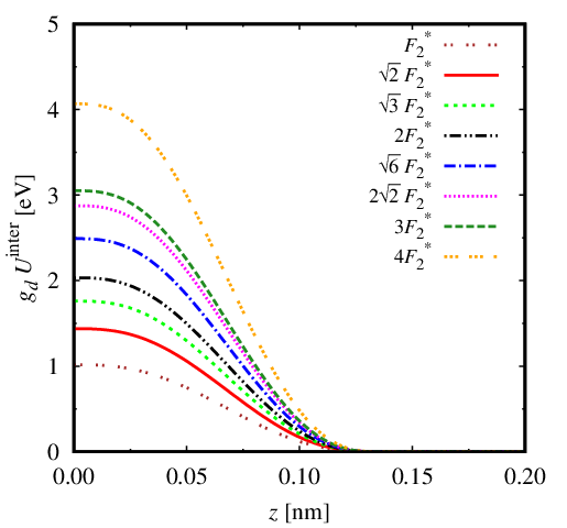
and they are completely short-ranged. In Fig. 6 we plot 8 such potentials along the zz direction, corresponding to the 8 distinct positive values of the parameters U{B}interU^{\rm inter}_{\{B\}} (see Tables 1, 2 and 3).

We emphasize that the relevance of interband and partially intraband potentials needs to be assessed according to their effect on the envelope functions. Indeed, despite their smaller energy scale with respect to fully intraband processes, interband transitions represent new channels for band mixing, whose effect might possibly be comparable to that of the magnetic field and spin-orbit coupling in strongly confined systems, such as quantum dots. In the context of Si-based quantum computing, where small amounts of band mixing can significantly affect the qubit functionalities, these contributions should also be included.

Refer to caption
Figure 1: Short-range contribution to the intraband potential W~B,B′,B′,B​(𝒓)\widetilde{W}_{B,B^{\prime},B^{\prime},B}(\bm{r}), along the direction 𝒓=(0,0,z)\bm{r}=(0,0,z). The energy splitting of the potentials corresponding to different values of B=(J,M)B=(J,M) and B′=(J′,M′)B^{\prime}=(J^{\prime},M^{\prime}) is apparent close to 𝒓=𝟎\bm{r}=\bm{0}. The three distinct values at 𝒓=𝟎\bm{r}=\bm{0} are F0F_{0} and F0±F2∗F_{0}\pm F_{2}^{*}, according to Eq. (30).
Refer to caption
Figure 2: Long-range contribution to the intraband potential W~B,B′,B′,B​(𝒓)\widetilde{W}_{B,B^{\prime},B^{\prime},B}(\bm{r}), along the direction 𝒓=(0,0,z)\bm{r}=(0,0,z). The differences in the curves are due to the different values taken by ΔB,B′(2)\Delta^{(2)}_{B,B^{\prime}} for different values of BB and B′B^{\prime}. Compare with Fig. 3.
Refer to caption
Figure 3: Long-range second-order correction to the full intraband potential W~B,B′,B′,B​(𝒓)\widetilde{W}_{B,B^{\prime},B^{\prime},B}(\bm{r}) in Eq. (72) along the direction 𝒓=(0,0,z)\bm{r}=(0,0,z), labelled by the band indexes B=(J,M)B=(J,M) and B′=(J′,M′)B^{\prime}=(J^{\prime},M^{\prime}).
Refer to caption
Figure 4: Short-range contribution to the partially intraband potential W~B,B′,B​",B​(𝒓)\widetilde{W}_{B,B^{\prime},B",B}(\bm{r}) in Eq. (73) along the direction 𝒓=(z,0,z)\bm{r}=(z,0,z), labelled by the band indexes, B=(J,M)B=(J,M) and B′=(J′,M′)B^{\prime}=(J^{\prime},M^{\prime}).
Refer to caption
Figure 5: Long-range contribution to the partially intraband potential W~B,B′,B​",B​(𝒓)\widetilde{W}_{B,B^{\prime},B",B}(\bm{r}) in Eq. (73) along the direction 𝒓=(z,0,z)\bm{r}=(z,0,z) for several selected transitions with J′=3/2J^{\prime}=3/2.
Refer to caption
Figure 6: Eight selected interband potentials, plotted along the direction 𝒓=(0,0,z)\bm{r}=(0,0,z), corresponding to the positive values of U{B}interU^{\rm inter}_{\{B\}}.

IX Numerical results

In order to illustrate the impact of interactions in Si QDs and quantify the role of short-range interactions, we now present the results of configuration-interaction calculations of the two-hole energy eigenvalues for three prototypical (harmonic) confinements. For a spatially slowly-varying confinement potential V⁡(𝒓)V(\bm{r}), the single-hole Hamiltonian is written according to the Lüttinger-Kohn 𝒌⋅𝒑\bm{k}\cdot\bm{p} formula LK; Voon_book; Secchi21,

HLK=H𝒌⋅𝒑+diag⁡[VQD​(𝒓)],\displaystyle H_{\rm LK}=H_{\bm{k}\cdot\bm{p}}+{\rm diag}\left[V_{\rm QD}(\bm{r})\right]\,, (75)

where H𝒌⋅𝒑H_{\bm{k}\cdot\bm{p}} is the 6-band 𝒌⋅𝒑\bm{k}\cdot\bm{p} kinetic-energy operator, and

VQD​(𝒓)=12​(κx​x2+κy​y2+κz​z2)\displaystyle V_{\rm QD}(\bm{r})=\frac{1}{2}\left(\kappa_{x}x^{2}+\kappa_{y}y^{2}+\kappa_{z}z^{2}\right) (76)

is a 3D harmonic potential, which models an anisotropic single QD confinement. Rather than to the spring constants κα\kappa_{\alpha}, with α∈{x,y,z}\alpha\in\{x,y,z\}, in the following we refer to the characteristic confinement lengths ℓα=ℏ​γ1/(m0​ωα)\ell_{\alpha}=\sqrt{\hbar\gamma_{1}/(m_{0}\omega_{\alpha})}, where γ1=4.285\gamma_{1}=4.285 is the first Lüttinger parameter for Si, m0m_{0} is the bare electron mass, and ωα=κα​γ1/m0\omega_{\alpha}=\sqrt{\kappa_{\alpha}\gamma_{1}/m_{0}}.

We consider three QDs (QD1, QD2, and QD3), specified by the following confinement lengths ℓ=(ℓx,ℓy,ℓz)\bm{\ell}=(\ell_{x},\ell_{y},\ell_{z}):

QD1:ℓ1=(20,2,2)​nm,\displaystyle{\rm QD1:}\quad\bm{\ell}_{1}=(20,2,2)\,\,{\rm nm}\,,
QD2:ℓ2=(10,4,2)​nm,\displaystyle{\rm QD2:}\quad\bm{\ell}_{2}=(10,4,2)\,\,{\rm nm}\,,
QD3:ℓ3=(4,4,4)​nm.\displaystyle{\rm QD3:}\quad\bm{\ell}_{3}=(4,4,4)\,\,{\rm nm}\,. (77)

The characteristic energy scale associated with a harmonic confinement is the effective frequency ωα∗=κα/m∗\omega^{*}_{\alpha}=\sqrt{\kappa_{\alpha}/m^{*}}, where m∗m^{*} is the effective mass of the confined particles. In a multiband system, the definition of the effective mass is not trivial; we consider here m∗=(γ1+52​γ2)​m0m^{*}=\left(\gamma_{1}+\frac{5}{2}\gamma_{2}\right)m_{0}, which is the isotropic part of the effective mass tensor for the light/heavy-hole subsystem Voon_book. The energy quanta ℏ​ωα∗\hbar\omega^{*}_{\alpha} corresponding to the considered values of ℓα\ell_{\alpha} are:

ℓα=2​nm⇒ℏ​ωα∗=89.337​meV,\displaystyle\ell_{\alpha}=2\,\,{\rm nm}\,\,\,\Rightarrow\hbar\omega^{*}_{\alpha}=89.337\,\,{\rm meV}\,,
ℓα=4​nm⇒ℏ​ωα∗=22.334​meV,\displaystyle\ell_{\alpha}=4\,\,{\rm nm}\,\,\,\Rightarrow\hbar\omega^{*}_{\alpha}=22.334\,\,{\rm meV}\,,
ℓα=10​nm⇒ℏ​ωα∗=3.573​meV,\displaystyle\ell_{\alpha}=10\,\,{\rm nm}\,\,\,\Rightarrow\hbar\omega^{*}_{\alpha}=3.573\,\,{\rm meV}\,,
ℓα=20​nm⇒ℏ​ωα∗=0.893​meV.\displaystyle\ell_{\alpha}=20\,\,{\rm nm}\,\,\,\Rightarrow\hbar\omega^{*}_{\alpha}=0.893\,\,{\rm meV}\,. (78)

For each of the cases listed in (77), we study the impact of interactions (both short- and long- ranged) on the two-hole eigenvalues. The latter are obtained from the exact numerical diagonalization of the two-hole Hamiltonian, according to the general procedure that we have presented in Ref. Secchi21 for the study of double QDs. In that case, however, interband Coulomb interactions could be neglected because the two holes tend to localize in different dots, so their distance is always very large with respect to the typical range of interband interactions, which are all short-ranged. Since here we consider single QDs, with different confinement strengths, we include all the interaction processes derived above.

As can be expected, long- and short- range Coulomb interactions are in competition, and their interplay is affected by the strength of the confinement potential. Two qualitative pictures can be considered as a reference: 1) when the confinement is relatively weak, the long-range Coulomb repulsion causes the particles to localize far away from each other, forming a Wigner molecule (WM): in these situations the short-range interactions are completely negligible; 2) when the confinement is relatively strong, the two holes are constrained to be close to each other near the center of the QD, despite the Coulomb repulsion: in these situations, short-range interactions can play a role, which we quantify in the following.

Although the interaction potential derived by Vinsome and Richardson is appropriate for isolated bulk Si, we remark that, in a real device, the Si QD is embedded in a dielectric environment which can screen the long-range repulsion between holes. The precise form of the dielectric function is then device-specific. For the sake of generality, we here use the following form of the dielectric function,

ϵ(r)={(ϵ0−1)​rr0+1forr≤r0ϵ0forr>r0,\displaystyle\epsilon(r)=\left\{\begin{matrix}\left(\epsilon_{0}-1\right)\frac{r}{r_{0}}+1\quad{\rm for}\quad r\leq r_{0}\\ \epsilon_{0}\quad{\rm for}\quad r>r_{0}\end{matrix}\right.\,, (79)

which is very similar to the Vinsome-Richardson formula when the parameter r0=0.3r_{0}=0.3 nm, and it allows to perform a systematic study of the dependence of the eigenvalues on the screening. In particular, we study the evolution of the two-hole eigenvalues as a function of the parameter 1/ϵ01/\epsilon_{0} ranging from 0 (which suppresses the long-range interaction) to 0.0855, corresponding to the inverse dielectric constant of isolated bulk Si. Since the screening induced by the dielectric environment always increases the long-range screening, 1/ϵ01/\epsilon_{0} can never be higher than 0.0855 in a pure Si QD, and the range [0,0.0855][0,0.0855] covers all possible cases.

Refer to caption
Figure 7: Two-hole excitation energies for QD1 [see Eqs. (77)], as functions of 1/ϵ01/\epsilon_{0}. The ground state is a singlet; among the curves labelled with letters in the plot, (a) and (c) are triplets, while (b), (d) and (e) are singlets.
Refer to caption
Figure 8: Two-hole excitation energies for QD2 [see Eqs. (77)], as functions of 1/ϵ01/\epsilon_{0}. The ground state is a singlet; among the curves labelled with letters in the plot, (a) and (c) are triplets, while (b) is a singlet.
Refer to caption
Figure 9: Two-hole excitation energies for QD3 [see Eqs. (77)], as functions of 1/ϵ01/\epsilon_{0}. The ground manifold is made of 6 states, split by interactions on the scale of 10−110^{-1} meV in the fully interacting regime (see Table 8).
only SR non interacting fully interacting
Δ​Ea\Delta E_{\rm a} 0.7500.750 0.9000.900 0.0510.051
Δ​Eb\Delta E_{\rm b} 0.9070.907 0.9000.900 0.1230.123
Δ​Ec\Delta E_{\rm c} 1.6451.645 1.7941.794 0.0820.082
Δ​Ed\Delta E_{\rm d} 1.7411.741 1.7941.794 0.9590.959
Δ​Ee\Delta E_{\rm e} 1.8241.824 1.7991.799 1.1261.126
Table 6: Selected two-hole excitation energies (in meV) of QD1 [compare with Fig. 7], computed using the Vinsome-Richardson formula for the dielectric function. Here, Δ​Ex=Ex−E0\Delta E_{x}=E_{x}-E_{0}, where x∈{a,b,c,d,e}x\in\{{\rm a,b,c,d,e}\} and E0E_{0} is the ground energy.
only SR non interacting fully interacting
Δ​Ea\Delta E_{\rm a} 2.9312.931 3.1393.139 0.0660.066
Δ​Eb\Delta E_{\rm b} 3.1443.144 3.1393.139 3.0413.041
Δ​Ec\Delta E_{\rm c} 5.7295.729 5.8415.841 3.0913.091
Table 7: Selected two-hole excitation energies (in meV) of QD2 [compare with Fig. 8], computed using the Vinsome-Richardson formula for the dielectric function. Here, Δ​Ex=Ex−E0\Delta E_{x}=E_{x}-E_{0}, where x∈{a,b,c}x\in\{{\rm a,b,c}\} and E0E_{0} is the ground energy.

In general, interactions reduce the the two-hole excitation energies with respect to the non-interacting regime. The physical interpretation of the excitations changes from the progressive occupation of single-particle excited states (in the non-interacting case) to the vibrations of the charges around their classical equilibrium positions (in the Wigner-molecule case). The transition is a continuous one, since the system has a finite size.

IX.1 Quantum dot 1

QD1 is a quasi-1D system, because the confinement is much stronger in the (y,z)(y,z) plane than in the xx direction. The smallest energy scale associated with confinement is ℏ​ωx∗=0.893\hbar\omega^{*}_{x}=0.893 meV. The two-hole excitation energies are displayed in Fig. 7. Tracking the evolution of the eigenvalues as functions of 1/ϵ01/\epsilon_{0}, we see that

  • •

    At 1/ϵ0=01/\epsilon_{0}=0, the excitation energies Δ​Ex\Delta E_{x}, for the excitations x∈{a,b,c,d,e}x\in\{{\rm a,b,c,d,e}\}, can be approximately grouped into a quartet [made of triplet (a) and singlet (b)] and a quintet [made of triplet (c) and singlets (d) and (e)]. The internal splittings within the quartet and the quintet are due to the SR interactions (both intra- and inter-band), which are not suppressed by setting 1/ϵ0=01/\epsilon_{0}=0. In the non-interacting system, the internal splittings within the quartet and the quintet vanish (compare the first two columns of Table 6). This shows that, in a regime of high screening, SR interactions can be relevant; e.g., Δ​Eb−Δ​Ea=0.157\Delta E_{\rm b}-\Delta E_{\rm a}=0.157 meV at 1/ϵ0=01/\epsilon_{0}=0.

  • •

    Neglecting the splitting due to SR interactions (see the second column of Table 6), the energy separations between consecutive low-energy multiplets in the non-interacting regime are Δ​Ea=0.900\Delta E_{\rm a}=0.900 meV and Δ​Ec−Δ​Eb=0.894\Delta E_{\rm c}-\Delta E_{\rm b}=0.894 meV, which are compatible with ℏ​ωx∗\hbar\omega^{*}_{x}.

  • •

    As the long-range interaction is switched on (1/ϵ01/\epsilon_{0} increases), the singlet, the quartet, and three among the quintet states converge towards a common energy (apart from residual exchange interactions), while two of the quintet states join other, higher-energy states to form excited interacting multiplets. This reorganization of the spectrum when the interaction is fully switched on, and in particular the formation of highly degenerate manifolds, is a typical signature of the formation of a quasi-1D WM Secchi10; Corrigan21; Ercan21. The gap between the two lowest manifolds in the fully interacting regime (1/ϵ0=0.08551/\epsilon_{0}=0.0855) is given by Δ​Ed−Δ​Ea+Δ​Eb+Δ​Ec4=0.895\Delta E_{\rm d}-\frac{\Delta E_{\rm a}+\Delta E_{\rm b}+\Delta E_{\rm c}}{4}=0.895 meV (see the third column of Table 6), which is compatible with ℏ​ωx∗\hbar\omega^{*}_{x}, pointing to a center-of-mass excitation of the quasi-1D WM.

  • •

    At 1/ϵ0=0.08551/\epsilon_{0}=0.0855, intra-band interactions are negligible, i.e., the modification of the energy gaps in the third column of Table 6 when the intra-band terms are set to zero is <1​μ<1\mueV. This is consistent with the WM picture, because the intra-band interactions are all short-ranged and, therefore, are not expected to contribute significantly when the holes are localized far apart.

We notice that the evidence for WM formation in two-electron QDs in Si heterostructures has been reported in recent experimental and theoretical works Corrigan21; Ercan21.

IX.2 Quantum dot 2

We now consider the two-hole spectrum of QD2. In this case, the confinement is still stronger in the (y,z)(y,z) plane than in the xx direction, but the symmetry has been lowered (ℓy≠ℓz\ell_{y}\neq\ell_{z}) and ℓx\ell_{x} has been decreased with respect to QD1. The excitation energies are shown in Fig. 8. As in the case of QD1, we notice a characteristic reorganization of the spectrum as the LR interactions are turned on, which points to the formation of a WM. The degeneracies of the WM manifolds are smaller than in the case of QD1 because of the lower symmetry of the confinement potential. The excitation energy of the fifth eigenstate, Δ​Eb\Delta E_{\rm b}, evolves from 3.1443.144 meV (at 1/ϵ0=01/\epsilon_{0}=0) to 3.0413.041 meV (at 1/ϵ0=0.08551/\epsilon_{0}=0.0855), remaining always close to (but significantly smaller than) ℏ​ωx∗=3.573\hbar\omega^{*}_{x}=3.573 meV [see (78)]. In the fully interacting regime, this is reminiscent of a single center-of-mass excitation of a WM (inspection of the eigenstate confirms that it evolves from essentially a single Slater determinant of single-hole states at 1/ϵ0=01/\epsilon_{0}=0, to a strongly correlated state at 1/ϵ0=0.08551/\epsilon_{0}=0.0855). However, the dependence of Δ​Eb\Delta E_{\rm b} on 1/ϵ01/\epsilon_{0}, which would not occur in a one-band harmonic dot, signals a significant interplay between different vibrational modes induced by the non-triviality of the 6-band kinetic-energy operator. The excitation energies Δ​Ea\Delta E_{\rm a} and Δ​Ec\Delta E_{\rm c} of the two triplets singled out in Fig. 8 drop from 2.9312.931 meV to 0.0660.066 meV, and from 5.7295.729 meV to 3.0913.091 meV ≈ℏ​ωx∗\approx\hbar\omega^{*}_{x}, respectively, when moving from the fully screened to the fully interacting regime (see Table 7).

Analogously to the case of QD1, also in QD2 we observe that SR interactions are significant in the regime of high screening (e.g., Δ​Eb−Δ​Ea=0.213\Delta E_{\rm b}-\Delta E_{\rm a}=0.213 meV at 1/ϵ0=01/\epsilon_{0}=0), while they are negligible at 1/ϵ0=0.08551/\epsilon_{0}=0.0855, consistently with the interpretation of the unscreened spectrum in terms of the formation of a WM.

IX.3 Quantum dot 3

Finally, the two-hole spectrum of QD3 does not show any sign of the formation of a WM. In fact, in this case, confinement is very strong along all directions, overcoming the localizing effect of the Coulomb repulsion. The two-hole excitation energies of QD3 are shown in Fig. 9. The 6-fold quasi-degeneracy of the ground state manifold, independent of the strength of the LR interaction, is due to the high symmetry of the confinement potential. The SR interactions lift this degeneracy, which would be exact in the completely non-interacting regime. In the fully screened regime, 1/ϵ0=01/\epsilon_{0}=0, the degeneracy is lifted by the SR interactions on the scale of ≈101​μ\approx 10^{1}\mueV (see first column of Table 8). In this case, the LR interactions are responsible for a larger lifting, as shown in the second column of Table 8 for the fully interacting case. In this regime, the impact of interband interactions is on the scale of a few μ\mueV up to ≈15​μ\approx 15\mueV for the 5th excited state, as can be seen from the comparison between the second and the third columns of Table 8; the third column shows the excitation energies obtained when only the intraband interactions (both LR and SR) are included in the calculations.

only SR fully interacting only intraband
Δ​E1\Delta E_{1} 0.0140.014 0.1670.167 0.1650.165
Δ​E2\Delta E_{2} 0.0140.014 0.1670.167 0.1650.165
Δ​E3\Delta E_{3} 0.0140.014 0.1890.189 0.1890.189
Δ​E4\Delta E_{4} 0.0400.040 0.2990.299 0.2980.298
Δ​E5\Delta E_{5} 0.0420.042 0.3190.319 0.3040.304
Table 8: Excitation energies (in meV) of the first 5 two-hole excited states above the ground state in QD3 [compare with Fig. 9], computed using the Vinsome-Richardson formula for the dielectric function. When all interactions are neglected, all these gaps Δ​Ex=0\Delta E_{x}=0.

X Conclusions

In conclusion, we have thoroughly investigated the band scattering processes induced by the Coulomb interaction in a system of holes at the 𝚪\bm{\Gamma} point in Si, and derived the relevant potentials. In particular, a set of many previously overlooked interband and partially intraband processes has been derived, most of which are relevant at short length scales. Corrections to the long-range effective interaction, which is usually assumed to be a simple Coulomb intraband potential, have also been derived. Such corrections decay to zero quickly with the inter-hole distance.

We have performed CI calculations of the two-hole spectra in three exemplary QDs, including all interaction terms, in order to study the impact of long-range and short-range interactions. These calculations show that two holes embedded in realistic QDs in Si tend to form Wigner molecules, whose signature can be seen in the values and degeneracies of the excitation energies. A similar result had been reported for electrons in Si Corrigan21; Ercan21 but, to the best of our knowledge, not yet for holes. In our numerical calculations, the long-range interaction is gradually switched on by changing the value of the bulk dielectric function from the fully screened regime (1/ϵ0=01/\epsilon_{0}=0) to the fully interacting regime (1/ϵ0=0.08551/\epsilon_{0}=0.0855, the value for isolated bulk Si). Therefore, these calculations should qualitatively reproduce the spectra which can be obtained in the presence of a variable dielectric environment surrounding the Si QDs (e.g., that provided by close metallic gates). The impact of short-range interactions on two-hole spectra is found to be relevant mostly in the regime of high screening due to the dielectric environment, while it becomes essentially negligible in an isolated Si QD.

Acknowledgements.
The authors acknowledge financial support from the European Commission through the project IQubits (Call: H2020-FETOPEN-2018-2019-2020-01, Project ID: 829005). The authors acknowledge CINECA for HPC computing resources and support under the ISCRA initiative (IsC87 ESQUDO - HP10CXQWD5).

Appendix A Transformations involving the Clebsch-Gordan coefficients

The Clebsch-Gordan coefficients appearing in Eq. (4) are:

SB,α,σ\displaystyle S_{B,\alpha,\sigma}
=δJ,32[δM,σ​3212(δα,x+iσδα,y)−δM,σ​1223δα,z\displaystyle=\delta_{J,\frac{3}{2}}\Bigg[\delta_{M,\sigma\frac{3}{2}}\frac{1}{\sqrt{2}}(\delta_{\alpha,x}+{\rm i}\sigma\delta_{\alpha,y})-\delta_{M,\sigma\frac{1}{2}}\sqrt{\frac{2}{3}}\delta_{\alpha,z}
−δM,−σ​12σ6(δα,x−iσδα,y)]\displaystyle\quad-\delta_{M,-\sigma\frac{1}{2}}\frac{\sigma}{\sqrt{6}}\left(\delta_{\alpha,x}-{\rm i}\sigma\delta_{\alpha,y}\right)\Bigg]
+δJ,12​13​[δM,σ​12​δα,z−σ​δM,−σ​12​(δα,x−i​σ​δα,y)].\displaystyle\quad+\delta_{J,\frac{1}{2}}\frac{1}{\sqrt{3}}\Big[\delta_{M,\sigma\frac{1}{2}}\delta_{\alpha,z}-\sigma\delta_{M,-\sigma\frac{1}{2}}\left(\delta_{\alpha,x}-{\rm i}\sigma\delta_{\alpha,y}\right)\Big]\,. (80)

In the derivation of the effective band-dependent interaction potential, after substituting the expressions of the single-hole eigenstates |ν⟩|\nu\rangle [Eq. (5)] into Eq. (11), we obtain Eq. (12), with

W{B}\displaystyle W_{\{B\}} (𝒓−𝒓′)≡V⁡(𝒓−𝒓′)​1𝒩2​∑{𝑹}∑{j}(−1)j1+j2+j3+j4\displaystyle\left(\bm{r}-\bm{r}^{\prime}\right)\equiv V\left(\bm{r}-\bm{r}^{\prime}\right)\frac{1}{\mathcal{N}^{2}}\sum_{\{\bm{R}\}}\sum_{\{j\}}(-1)^{j_{1}+j_{2}+j_{3}+j_{4}}
×∑{α}∑σ,σ′(SB1,α1,σ∗​SB4,α4,σ)​(SB2,α2,σ′∗​SB3,α3,σ′)\displaystyle\quad\times\sum_{\{\alpha\}}\sum_{\sigma,\sigma^{\prime}}\left(S^{*}_{B_{1},\alpha_{1},\sigma}S_{B_{4},\alpha_{4},\sigma}\right)\left(S^{*}_{B_{2},\alpha_{2},\sigma^{\prime}}S_{B_{3},\alpha_{3},\sigma^{\prime}}\right)
×ϕpα1∗​(𝒓−𝑹1,j1)​ϕpα2∗​(𝒓′−𝑹2,j2)\displaystyle\quad\times\phi^{*}_{p_{\alpha_{1}}}(\bm{r}-\bm{R}_{1,j_{1}})\,\phi^{*}_{p_{\alpha_{2}}}(\bm{r}^{\prime}-\bm{R}_{2,j_{2}})
×ϕpα3​(𝒓′−𝑹3,j3)​ϕpα4​(𝒓−𝑹4,j4).\displaystyle\quad\times\phi_{p_{\alpha_{3}}}(\bm{r}^{\prime}-\bm{R}_{3,j_{3}})\,\phi_{p_{\alpha_{4}}}(\bm{r}-\bm{R}_{4,j_{4}})\,. (81)

Eq. (81) includes summations having the general form

∑σ(∑α′ϕpα′∗​(𝒙′)​SB′,(α′,σ)∗)​(∑αSB,(α,σ)​ϕpα​(𝒙)),\displaystyle\sum_{\sigma}\left(\sum_{\alpha^{\prime}}\phi^{*}_{p_{\alpha^{\prime}}}(\bm{x}^{\prime})S^{*}_{B^{\prime},(\alpha^{\prime},\sigma)}\right)\left(\sum_{\alpha}S_{B,(\alpha,\sigma)}\phi_{p_{\alpha}}(\bm{x})\right)\,, (82)

where 𝒙\bm{x} and 𝒙′\bm{x}^{\prime} denote, in general, two different positions. We perform the summation in Eq. (82), using Eq. (80), and expressing the result in terms of the orbitals given in Eq. (8). We obtain that the term involving the sum over α\alpha in Eq. (82) is

∑αSB,(α,σ)​ϕpα​(𝒓)\displaystyle\sum_{\alpha}S_{B,(\alpha,\sigma)}\phi_{p_{\alpha}}(\bm{r}) =δJ,32​δM,3​σ2​ϕσ​(𝒓)+YJ​δM,σ2​ϕ0​(𝒓)\displaystyle=\delta_{J,\frac{3}{2}}\delta_{M,\frac{3\sigma}{2}}\phi_{\sigma}(\bm{r})+Y_{J}\,\delta_{M,\frac{\sigma}{2}}\phi_{0}(\bm{r})
−σ​XJ​δM,−σ2​ϕ−σ​(𝒓),\displaystyle\quad-\sigma X_{J}\,\delta_{M,-\frac{\sigma}{2}}\phi_{-\sigma}(\bm{r})\,, (83)

where σ∈{+1,−1}\sigma\in\{+1,-1\}, and

XJ≡13​(2​δJ,12+δJ,32),\displaystyle X_{J}\equiv\frac{1}{\sqrt{3}}\left(\sqrt{2}\delta_{J,\frac{1}{2}}+\delta_{J,\frac{3}{2}}\right)\,,
YJ≡13​(δJ,12−δJ,32​2).\displaystyle Y_{J}\equiv\frac{1}{\sqrt{3}}\left(\delta_{J,\frac{1}{2}}-\delta_{J,\frac{3}{2}}\sqrt{2}\right)\,. (84)

The term involving the sum over α′\alpha^{\prime} from Eq. (82) is obtained by taking the complex conjugate of Eq. (83) and changing the indices. We finally write

∑α′,α,σϕpα′∗​(𝒙′)​SB′,(α′,σ)∗​SB,(α,σ)​ϕpα​(𝒙)\displaystyle\sum_{\alpha^{\prime},\alpha,\sigma}\phi^{*}_{p_{\alpha^{\prime}}}(\bm{x}^{\prime})S^{*}_{B^{\prime},(\alpha^{\prime},\sigma)}S_{B,(\alpha,\sigma)}\phi_{p_{\alpha}}(\bm{x})
≡∑m′,mϕm′∗​(𝒙′)​FB′,Bm′,m​ϕm​(𝒙),\displaystyle\equiv\sum_{m^{\prime},m}\phi^{*}_{m^{\prime}}(\bm{x}^{\prime})\,F^{m^{\prime},m}_{B^{\prime},B}\,\phi_{m}(\bm{x})\,, (85)

where we have introduced the matrix FB′,Bm′,mF^{m^{\prime},m}_{B^{\prime},B}, with elements

FB′,B±1,±1=(δJ′,32​δJ,32​δM,±32+XJ′​XJ​δM,±12)​δM′,M,\displaystyle F_{B^{\prime},B}^{\pm 1,\pm 1}=\Big(\delta_{J^{\prime},\frac{3}{2}}\,\delta_{J,\frac{3}{2}}\,\delta_{M,\pm\frac{3}{2}}+X_{J^{\prime}}\,X_{J}\,\delta_{M,\pm\frac{1}{2}}\Big)\delta_{M^{\prime},M}\,, (86)
FB′,B±1,0=δJ′,32​δM′,±32​YJ​δM,±12±XJ′​δM′,±12​YJ​δM,∓12,\displaystyle F_{B^{\prime},B}^{\pm 1,0}=\delta_{J^{\prime},\frac{3}{2}}\,\delta_{M^{\prime},\pm\frac{3}{2}}\,Y_{J}\,\delta_{M,\pm\frac{1}{2}}\pm X_{J^{\prime}}\,\delta_{M^{\prime},\pm\frac{1}{2}}\,Y_{J}\,\delta_{M,\mp\frac{1}{2}}\,, (87)
FB′,B0,±1=YJ′​δM′,±12​δJ,32​δM,±32±YJ′​δM′,∓12​XJ​δM,±12,\displaystyle F_{B^{\prime},B}^{0,\pm 1}=Y_{J^{\prime}}\,\delta_{M^{\prime},\pm\frac{1}{2}}\,\delta_{J,\frac{3}{2}}\,\delta_{M,\pm\frac{3}{2}}\pm Y_{J^{\prime}}\,\delta_{M^{\prime},\mp\frac{1}{2}}\,X_{J}\,\delta_{M,\pm\frac{1}{2}}\,, (88)
FB′,B±1,∓1\displaystyle F_{B^{\prime},B}^{\pm 1,\mp 1} =∓δJ′,32​δM′,±32​XJ​δM,∓12\displaystyle=\mp\,\delta_{J^{\prime},\frac{3}{2}}\,\delta_{M^{\prime},\pm\frac{3}{2}}\,X_{J}\,\delta_{M,\mp\frac{1}{2}}
±XJ′​δM′,±12​δJ,32​δM,∓32,\displaystyle\quad\pm X_{J^{\prime}}\,\delta_{M^{\prime},\pm\frac{1}{2}}\,\delta_{J,\frac{3}{2}}\,\delta_{M,\mp\frac{3}{2}}\,, (89)
FB′,B0,0=YJ′​YJ​δM′,M​δ|M′|,12.\displaystyle F_{B^{\prime},B}^{0,0}=Y_{J^{\prime}}\,Y_{J}\,\delta_{M^{\prime},M}\,\delta_{|M^{\prime}|,\frac{1}{2}}\,. (90)

The matrix FF has the following trace property:

∑mFB′,Bm,m=δB′,B,\displaystyle\sum_{m}F^{m,m}_{B^{\prime},B}=\delta_{B^{\prime},B}\,, (91)

as can be easily derived after noticing that

XJ′​XJ+YJ′​YJ=δJ′,J.\displaystyle X_{J^{\prime}}\,X_{J}+Y_{J^{\prime}}\,Y_{J}=\delta_{J^{\prime},J}\,. (92)

By applying Eq. (85) to Eq. (81), we obtain Eq. (13).

Appendix B Screened potential

We here discuss the explicit expression of the screened Coulomb potential V⁡(𝒓−𝒓′)V(\bm{r}-\bm{r}^{\prime}) in Si, which enters Eq. (13). The screened Coulomb interaction potential between two holes at distance rr reads

V⁡(r)=e2ϵ⁡(r)​r≡VC​(r)ϵ⁡(r),\displaystyle V(r)=\frac{e^{2}}{\epsilon(r)\,r}\equiv\frac{V_{\rm C}(r)}{\epsilon(r)}\,, (93)

where ϵ⁡(r)\epsilon(r) is a static, isotropicPhillips61 but nonhomogeneous dielectric function for Si, and VC​(r)=e2/rV_{\rm C}(r)=e^{2}/r is the bare Coulomb potential.

The modelling of ϵ⁡(r)\epsilon(r) has a long historyBassaniIadonisiPreziosi, from the semiclassical Thomas-Fermi theoryResta77; Chandramohan90; Franceschetti05, to quantum-mechanical models with simplifying assumptions on the band structurePenn62; Srinivasan68, to more refined numerical calculations based on empirical pseudo-potential methodsNara65; Nara66; Vinsome71; Richardson71. The numerical approaches account for material-specific details, such as the crystal band structure and the correct electronic dispersion, thus allowing for a description of the optical properties of materials which is more precise than that provided by analytical models. Moreover, they predict the bulk value ϵ0≡ϵ⁡(r→∞)\epsilon_{0}\equiv\epsilon(r\rightarrow\infty) of the dielectric function.

Numerical calculations are usually supplemented by interpolation functions, and thus lead to analytical expressions for ϵ⁡(r)\epsilon(r). We take as a reference the works of Vinsome and RichardsonVinsome71; Richardson71 on a comprehensive set of zincblende semiconductors. They perform large-scale RPA calculations (in reciprocal space), and they interpolate their numerical results with the following formula, valid in direct space:

ϵ(r)=(1ϵ0+λ1e−2πα1r/a+λ2e−2πα2r/a)−1,\displaystyle\epsilon(r)=\left(\frac{1}{\epsilon_{0}}+\lambda_{1}{\rm e}^{-2\pi\alpha_{1}r/a}+\lambda_{2}{\rm e}^{-2\pi\alpha_{2}r/a}\right)^{-1}\,, (94)

where aa is the cubic cell edge, and the fitting parameters for Si are written asRichardson71

1ϵ0≡BD,α1,2≡(C∓C2−4​D2)1/2,\displaystyle\frac{1}{\epsilon_{0}}\equiv\frac{B}{D}\,,\quad\quad\alpha_{1,2}\equiv\left(\frac{C\mp\sqrt{C^{2}-4D}}{2}\right)^{1/2}\,,
λ1,2≡12​(1−1ϵ0)±A−C2​(1+1ϵ0)C2−4​D,\displaystyle\lambda_{1,2}\equiv\frac{1}{2}\left(1-\frac{1}{\epsilon_{0}}\right)\pm\frac{A-\frac{C}{2}\left(1+\frac{1}{\epsilon_{0}}\right)}{\sqrt{C^{2}-4D}}\,, (95)

in terms of the quantities

A=0.34,B=0.016,C=2.6,D=0.17.\displaystyle A=0.34\,,\quad B=0.016\,,\quad C=2.6\,,\quad D=0.17\,. (96)

The bulk limit for the dielectric function according to Eq. (96) is ϵ0=10.625\epsilon_{0}=10.625. By modifying the value of BB to 0.014530.01453, one obtains ϵ0=11.7\epsilon_{0}=11.7, consistently with experimental dataDunlap53. The potential V⁡(r)V(r) is plotted in Fig. 10.

Refer to caption
Figure 10: Left vertical axis: Screened potential V⁡(r)V(r) with ϵ⁡(r)\epsilon(r) given by Eq. (94) (solid black curve), and Coulomb potential screened at all rr by the bulk dielectric constant ϵ0\epsilon_{0} (dashed blue curve), plotted for comparison. Right vertical axis: Dielectric function ϵ⁡(r)\epsilon(r), according to Eq. (94).

The explicit expressions for the quantities ℒ−2​(r)\mathcal{L}^{-2}(r) and ℳ−2​(r)\mathcal{M}^{-2}(r), contributing to the second-order correction to the long-range effective potentials [see Eqs. (50) and (51)], are

ℳ−2(r)=1r2+ϵ⁡(r)r2​πa∑n=12λnαne−2παnr/a,\displaystyle\mathcal{M}^{-2}(r)=\frac{1}{r^{2}}+\frac{\epsilon(r)}{r}\frac{2\pi}{a}\sum_{n=1}^{2}\lambda_{n}\alpha_{n}{\rm e}^{-2\pi\alpha_{n}r/a}\,, (97)

and

ℒ−2(r)≡3ℳ−2(r)+ϵ(r)4​π2a2∑n=12λnαn2e−2παnr/a.\displaystyle\mathcal{L}^{-2}(r)\equiv 3\mathcal{M}^{-2}(r)+\epsilon(r)\frac{4\pi^{2}}{a^{2}}\sum_{n=1}^{2}\lambda_{n}\alpha^{2}_{n}{\rm e}^{-2\pi\alpha_{n}r/a}\,. (98)

Appendix C Rüdenberg approach for multi-center integrals

A possible way to go beyond the two-center integral approximation can be outlined as follows. Following RüdenbergRudenberg51, we introduce a complete set of orthonormal orbitals centered at each atomic site 𝑹j\bm{R}_{j}:

{|χ,𝑹j⟩,χ=1s,…3p1,3p0,3p−1,…}.\displaystyle\Big\{\big|\chi,\bm{R}_{j}\big>\,,\quad\chi=1s,\ldots 3p_{1},3p_{0},3p_{-1},\ldots\Big\}\,. (99)

We define the overlap between orbitals centered at different atomic sites:

𝒪χ,χ′​(𝑹j,𝑹j′′)≡⟨χ,𝑹j|χ′,𝑹j′′⟩.\displaystyle\mathcal{O}_{\chi\,,\,\chi^{\prime}}\left(\bm{R}_{j},\bm{R}^{\prime}_{j^{\prime}}\right)\equiv\big<\chi,\bm{R}_{j}\big|\chi^{\prime},\bm{R}^{\prime}_{j^{\prime}}\big>\,. (100)

Due to the completeness of the set centered at any arbitrary site, we can expand the orbital centered at one site in terms of the orbitals centered at another site. According to Rüdenberg, at least if 𝑹\bm{R} and 𝑹′\bm{R}^{\prime} are very close, it can be assumed that the only relevant contribution in the expansion of an orbital ϕm​(𝒓−𝑹j′′)\phi_{m}(\bm{r}-\bm{R}_{j^{\prime}}^{\prime}) is the one from ϕm​(𝒓−𝑹j)\phi_{m}(\bm{r}-\bm{R}_{j}).

A possible way to refine this approximation is to consider instead the full set of 3​p3p orbitals (i.e., we allow χ\chi to be equal not just to m′m^{\prime}, but to any of the basis orbitals). Extending this to arbitrary atomic positions, one obtains for the interaction potential [Eq. (13)] the following expression:

W{M}​(𝒓−𝒓′)\displaystyle W_{\{M\}}\left(\bm{r}-\bm{r}^{\prime}\right)
≈V⁡(𝒓−𝒓′)​1𝒩2​∑𝑹,𝑹′∑j,j′∑{m}ΔM1,M4m1,m4​(𝑹j)\displaystyle\approx V\left(\bm{r}-\bm{r}^{\prime}\right)\frac{1}{\mathcal{N}^{2}}\sum_{\bm{R},\bm{R}^{\prime}}\sum_{j,j^{\prime}}\sum_{\{m\}}\Delta^{m_{1},m_{4}}_{M_{1},M_{4}}\left(\bm{R}_{j}\right)
×ΔM2,M3m2,m3​(𝑹j′′)​ϕm1∗​(𝒓−𝑹j)​ϕm2∗​(𝒓′−𝑹j′′)\displaystyle\quad\times\Delta^{m_{2},m_{3}}_{M_{2},M_{3}}\left(\bm{R}^{\prime}_{j^{\prime}}\right)\,\phi^{*}_{m_{1}}(\bm{r}-\bm{R}_{j})\,\phi^{*}_{m_{2}}(\bm{r}^{\prime}-\bm{R}^{\prime}_{j^{\prime}})
×ϕm3​(𝒓′−𝑹j′′)​ϕm4​(𝒓−𝑹j).\displaystyle\quad\times\phi_{m_{3}}(\bm{r}^{\prime}-\bm{R}^{\prime}_{j^{\prime}})\,\phi_{m_{4}}(\bm{r}-\bm{R}_{j})\,. (101)

where we have introduced the overlap form factor,

ΔM1,M4m1,m4​(𝑹j)\displaystyle\Delta^{m_{1},m_{4}}_{M_{1},M_{4}}\left(\bm{R}_{j}\right)
≡12∑𝑹′′,j′′(−1)j+j′′∑m5[FM1,M4m5,m4𝒪m5,m1(𝑹j′′′′,𝑹j)\displaystyle\equiv\frac{1}{2}\sum_{\bm{R}^{\prime\prime},j^{\prime\prime}}(-1)^{j+j^{\prime\prime}}\sum_{m_{5}}\Big[F_{M_{1},M_{4}}^{m_{5},m_{4}}\mathcal{O}_{m_{5},m_{1}}\left(\bm{R}^{\prime\prime}_{j^{\prime\prime}},\bm{R}_{j}\right)
+FM1,M4m1,m5𝒪m4,m5(𝑹j,𝑹j′′′′)].\displaystyle\quad+F_{M_{1},M_{4}}^{m_{1},m_{5}}\mathcal{O}_{m_{4},m_{5}}\left(\bm{R}_{j},\bm{R}^{\prime\prime}_{j^{\prime\prime}}\right)\Big]\,. (102)

The Rüdenberg approximation is recovered by assuming

𝒪m4,m5​(𝑹j,𝑹j′′′′)≈δm4,m5​𝒪m4,m4​(𝑹j,𝑹j′′′′),\displaystyle\mathcal{O}_{m_{4},m_{5}}\left(\bm{R}_{j},\bm{R}^{\prime\prime}_{j^{\prime\prime}}\right)\approx\delta_{m_{4},m_{5}}\mathcal{O}_{m_{4},m_{4}}\left(\bm{R}_{j},\bm{R}^{\prime\prime}_{j^{\prime\prime}}\right)\,, (103)

which yields

ΔM1,M4m1,m4​(𝑹j)\displaystyle\Delta^{m_{1},m_{4}}_{M_{1},M_{4}}\left(\bm{R}_{j}\right)
≈FM1,M4m1,m412∑𝑹′′,j′′(−1)j+j′′[𝒪m1,m1(𝑹j′′′′,𝑹j)\displaystyle\approx F_{M_{1},M_{4}}^{m_{1},m_{4}}\frac{1}{2}\sum_{\bm{R}^{\prime\prime},j^{\prime\prime}}(-1)^{j+j^{\prime\prime}}\Big[\mathcal{O}_{m_{1},m_{1}}\left(\bm{R}^{\prime\prime}_{j^{\prime\prime}},\bm{R}_{j}\right)
+𝒪m4,m4(𝑹j,𝑹j′′′′)].\displaystyle\quad+\mathcal{O}_{m_{4},m_{4}}\left(\bm{R}_{j},\bm{R}^{\prime\prime}_{j^{\prime\prime}}\right)\Big]\,. (104)

The two-center integral approximation is formally recovered by replacing

𝒪m,m​(𝑹j,𝑹j′′)→δ𝑹,𝑹′​δj,j′,\displaystyle\mathcal{O}_{m,m}\left(\bm{R}_{j},\bm{R}^{\prime}_{j^{\prime}}\right)\rightarrow\delta_{\bm{R},\bm{R}^{\prime}}\delta_{j,j^{\prime}}\,, (105)

which yields

ΔM1,M4m1,m4​(𝑹j)→FM1,M4m1,m4.\displaystyle\Delta^{m_{1},m_{4}}_{M_{1},M_{4}}\left(\bm{R}_{j}\right)\rightarrow F_{M_{1},M_{4}}^{m_{1},m_{4}}\,. (106)

Thus, we have seen that a possible strategy for improving over the two-center approximation requires the calculation of the quantity (102). We notice that, in a lattice,

𝒪χ,m′​(𝑹j,𝑹j′′)=𝒪χ,m′​(𝑹−𝑹′,j−j′),\displaystyle\mathcal{O}_{\chi,m^{\prime}}\left(\bm{R}_{j},\bm{R}^{\prime}_{j^{\prime}}\right)=\mathcal{O}_{\chi,m^{\prime}}\left(\bm{R}-\bm{R}^{\prime};j-j^{\prime}\right)\,, (107)

therefore, ΔM1,M4m1,m4​(𝑹j)\Delta^{m_{1},m_{4}}_{M_{1},M_{4}}\left(\bm{R}_{j}\right) is actually independent of 𝑹j\bm{R}_{j}:

ΔM1,M4m1,m4\displaystyle\Delta^{m_{1},m_{4}}_{M_{1},M_{4}}
≡12∑j′′(−1)j+j′′∑m5{FM1,M4m5,m4∑𝑹′′𝒪m5,m1(𝑹′′;j′′−j)\displaystyle\equiv\frac{1}{2}\sum_{j^{\prime\prime}}(-1)^{j+j^{\prime\prime}}\sum_{m_{5}}\Big\{F_{M_{1},M_{4}}^{m_{5},m_{4}}\sum_{\bm{R}^{\prime\prime}}\mathcal{O}_{m_{5},m_{1}}\left(\bm{R}^{\prime\prime};j^{\prime\prime}-j\right)
+FM1,M4m1,m5∑𝑹′′𝒪m4,m5(𝑹′′;j−j′′)}.\displaystyle\quad+F_{M_{1},M_{4}}^{m_{1},m_{5}}\sum_{\bm{R}^{\prime\prime}}\mathcal{O}_{m_{4},m_{5}}\left(\bm{R}^{\prime\prime};j-j^{\prime\prime}\right)\Big\}\,. (108)

Appendix D Derivation of the Hubbard parameters

D.1 General remarks

We rewrite Eq. (20) here in a more general way as

Ui,j,k,l\displaystyle U_{i,j,k,l} =∫d​𝒓1​∫d​𝒓2​ϕi∗​(𝒓1)​ϕj∗​(𝒓2)​VC​(|𝒓1−𝒓2|)\displaystyle=\int d\bm{r}_{1}\int d\bm{r}_{2}\,\phi^{*}_{i}(\bm{r}_{1})\phi^{*}_{j}(\bm{r}_{2})V_{\rm C}(|\bm{r}_{1}-\bm{r}_{2}|)
×ϕk​(𝒓2)​ϕl​(𝒓1),\displaystyle\quad\times\phi_{k}(\bm{r}_{2})\phi_{l}(\bm{r}_{1})\,, (109)

where the atomic orbital ϕi\phi_{i} is separable into the product of a radial part and a spherical harmonic,

ϕi​(𝒓)=Rni,li​(r)​Θli,mi​(θ)​Φmi​(φ),\displaystyle\phi_{i}(\bm{r})=R_{n_{i},l_{i}}(r)\,\Theta_{l_{i},m_{i}}(\theta)\,\Phi_{m_{i}}(\varphi)\,, (110)

where Slater29

Φm​(φ)=12​π​ei​m​φ,\displaystyle\Phi_{m}(\varphi)=\frac{1}{\sqrt{2\pi}}{\rm e}^{{\rm i}m\varphi}\,, (111)
Θl,m​(θ)=(2​l+1)2​(l−|m|)!(l+|m|)!​Pl,|m|​(cos⁡θ),\displaystyle\Theta_{l,m}(\theta)=\sqrt{\frac{(2l+1)}{2}\frac{(l-|m|)!}{(l+|m|)!}}P_{l,|m|}(\cos\theta)\,, (112)
Pl,|m|​(cos⁡θ)=12l​l!​sin|m|⁡θ​d|m|+l​(−sin2⁡θ)ld​(cos⁡θ)|m|+l.\displaystyle P_{l,|m|}(\cos\theta)=\frac{1}{2^{l}l!}\sin^{|m|}\theta\frac{d^{|m|+l}(-\sin^{2}\theta)^{l}}{d(\cos\theta)^{|m|+l}}\,. (113)

In the definition of the spherical harmonics, we have followed the convention adopted in Ref. Voon_book, i.e. the Condon-Shortley phase (−1)m(-1)^{m} for m≥0m\geq 0 is not included.

We then use the expansion of the Coulomb potential in series of Legendre polynomials, Eq. (23). After substituting it into Eq. (109), and performing some standard manipulations that involve the spherical harmonic addition theoremGriffith, we obtain

Ui,j,k,l\displaystyle U_{i,j,k,l} =δmi+mj,mk+ml​∑ℓ=0∞Rℓ​(ni,li,nj,lj,nk,lk,nl,ll)\displaystyle=\delta_{m_{i}+m_{j},m_{k}+m_{l}}\sum_{\ell=0}^{\infty}R_{\ell}(n_{i},l_{i};n_{j},l_{j};n_{k},l_{k};n_{l},l_{l})
×cℓ​(li,mi,ll,ml)​cℓ​(lk,mk,lj,mj),\displaystyle\quad\times c_{\ell}(l_{i},m_{i};l_{l},m_{l})\,c_{\ell}(l_{k},m_{k};l_{j},m_{j})\,, (114)

where

Rℓ​(ni,li,nj,lj,nk,lk,nl,ll)\displaystyle R_{\ell}\left(n_{i},l_{i};n_{j},l_{j};n_{k},l_{k};n_{l},l_{l}\right)
=e2​∫0∞d​r1​r12​∫0∞d​r2​r22​Rni,li​(r1)​Rnj,lj​(r2)​r<ℓr>ℓ+1\displaystyle=e^{2}\int_{0}^{\infty}dr_{1}r_{1}^{2}\int_{0}^{\infty}dr_{2}r_{2}^{2}\,R_{n_{i},l_{i}}(r_{1})R_{n_{j},l_{j}}(r_{2})\frac{r_{<}^{\ell}}{r_{>}^{\ell+1}}
×Rnk,lk​(r2)​Rnl,ll​(r1),\displaystyle\quad\times R_{n_{k},l_{k}}(r_{2})R_{n_{l},l_{l}}(r_{1})\,, (115)

and

cℓ​(l,m,l′,m′)\displaystyle c_{\ell}(l,m;l^{\prime},m^{\prime}) =22​ℓ+1​∫0πd​θ​sin⁡(θ)​Θl,m​(θ)\displaystyle=\sqrt{\frac{2}{2\ell+1}}\int_{0}^{\pi}d\theta\sin(\theta)\,\Theta_{l,m}(\theta)
×Θℓ,m−m′​(θ)​Θl′,m′​(θ).\displaystyle\quad\times\Theta_{\ell,m-m^{\prime}}(\theta)\,\Theta_{l^{\prime},m^{\prime}}(\theta)\,. (116)

This quantity vanishes unless

ℓ+l+l′​is​even∧|l−l′|≤ℓ≤l+l′.\displaystyle\ell+l+l^{\prime}\,\,{\rm is\,\,even}\quad\land\quad|l-l^{\prime}|\leq\ell\leq l+l^{\prime}\,. (117)

D.2 Valence orbitals in Silicon

In this work, we need only considering the case of

ni=nj=nk=nl=3,li=lj=lk=ll=1,\displaystyle n_{i}=n_{j}=n_{k}=n_{l}=3\,,\quad l_{i}=l_{j}=l_{k}=l_{l}=1\,, (118)

since we are only concerned with 3​p3p atomic orbitals. From the condition Eq. (117), we then see that the only nonvanishing terms in Eq. (114) are those with ℓ∈{0,2}\ell\in\{0,2\}.

Since nn and ll are fixed, we restore the notation of Eq. (20), where only the mm numbers are specified explicitly. Analogously, we put cℓ​(1,m,1,m′)≡cℓ​(m,m′)c_{\ell}(1,m;1,m^{\prime})\equiv c_{\ell}(m,m^{\prime}). We also introduce the Slater-Condon parameters

F0​(3​p,3​p)\displaystyle F_{0}(3p,3p) ≡F0≡R0​(3,1,3,1,3,1,3,1)\displaystyle\equiv F_{0}\equiv R_{0}(3,1;3,1;3,1;3,1)
=e2​∫0∞d​r1​r12​∫0∞d​r2​r22​1r>​R3,12​(r1)​R3,12​(r2),\displaystyle=e^{2}\!\int_{0}^{\infty}dr_{1}r_{1}^{2}\int_{0}^{\infty}dr_{2}r_{2}^{2}\,\frac{1}{r_{>}}\,R^{2}_{3,1}(r_{1})R^{2}_{3,1}(r_{2})\,,
F2​(3​p,3​p)\displaystyle F_{2}(3p,3p) ≡F2≡R2​(3,1,3,1,3,1,3,1)\displaystyle\equiv F_{2}\equiv R_{2}(3,1;3,1;3,1;3,1)
=e2​∫0∞d​r1​r12​∫0∞d​r2​r22​r<2r>3​R3,12​(r1)​R3,12​(r2),\displaystyle=e^{2}\!\int_{0}^{\infty}dr_{1}r_{1}^{2}\int_{0}^{\infty}dr_{2}r_{2}^{2}\,\frac{r^{2}_{<}}{r^{3}_{>}}R^{2}_{3,1}(r_{1})R^{2}_{3,1}(r_{2})\,, (119)

where r<=min​(r1,r2)r_{<}=\text{min}(r_{1},r_{2}) and r>=max​(r1,r2)r_{>}=\text{max}(r_{1},r_{2}). The quantities (119) coincide with those introduced in Eq. (25). The Hubbard parameters in Eq. (20) are then reduced to

U{m}\displaystyle U_{\{m\}} =δm1+m2,m3+m4[F0c0(m1,m4)c0(m3,m2)\displaystyle=\delta_{m_{1}+m_{2},m_{3}+m_{4}}\Big[F_{0}\,c_{0}(m_{1},m_{4})\,c_{0}(m_{3},m_{2})
+F2c2(m1,m4)c2(m3,m2)].\displaystyle\quad+F_{2}\,c_{2}(m_{1},m_{4})\,c_{2}(m_{3},m_{2})\Big]\,. (120)

We evaluate c0​(m,m′)c_{0}(m,m^{\prime}) and c2​(m,m′)c_{2}(m,m^{\prime}) analytically, using Eqs. (112) and (113). We obtain

c0​(m,m′)=δm,m′,\displaystyle c_{0}(m,m^{\prime})=\delta_{m,m^{\prime}}\,, (121)

and

c2​(m,m′)\displaystyle c_{2}(m,m^{\prime}) =δm,m′​(−1)|m|​(2−|m|)5\displaystyle=\delta_{m,m^{\prime}}\frac{(-1)^{|m|}\left(2-|m|\right)}{5}
+(1−δm,m′)​3​(|m|+|m′|)5.\displaystyle\quad+(1-\delta_{m,m^{\prime}})\frac{\sqrt{3\left(|m|+|m^{\prime}|\right)}}{5}\,. (122)

After substituting Eq. (122) into Eq. (120), we obtain Eq. (24).

Appendix E Derivation of the short-range potentials

Using Eqs. (26), we rewrite Eq. (19) as

W{B}SR​(𝑹j,𝑹j′′)\displaystyle W^{\rm SR}_{\{B\}}(\bm{R}_{j},\bm{R}^{\prime}_{j^{\prime}})
=δ𝑹j,𝑹j′′{FB1,B40,0FB2,B30,0U0,0,0,0\displaystyle=\delta_{\bm{R}_{j},\bm{R}^{\prime}_{j^{\prime}}}\Big\{F^{0,0}_{B_{1},B_{4}}\,F^{0,0}_{B_{2},B_{3}}U_{0,0,0,0}
+(FB1,B41,1+FB1,B4−1,−1)​(FB2,B31,1+FB2,B3−1,−1)​U1,1,1,1\displaystyle\quad+\Big(F^{1,1}_{B_{1},B_{4}}+F^{-1,-1}_{B_{1},B_{4}}\Big)\Big(F^{1,1}_{B_{2},B_{3}}+F^{-1,-1}_{B_{2},B_{3}}\Big)U_{1,1,1,1}
+[(FB1,B41,1+FB1,B4−1,−1)FB2,B30,0\displaystyle\quad+\Big[\Big(F^{1,1}_{B_{1},B_{4}}+F^{-1,-1}_{B_{1},B_{4}}\Big)F^{0,0}_{B_{2},B_{3}}
+FB1,B40,0(FB2,B31,1+FB2,B3−1,−1)]U1,0,0,1\displaystyle\quad+F^{0,0}_{B_{1},B_{4}}\Big(F^{1,1}_{B_{2},B_{3}}+F^{-1,-1}_{B_{2},B_{3}}\Big)\Big]U_{1,0,0,1}
+(FB1,B41,−1​FB2,B3−1,1+FB1,B4−1,1​FB2,B31,−1)​U1,−1,1,−1\displaystyle\quad+\Big(F^{1,-1}_{B_{1},B_{4}}\,F^{-1,1}_{B_{2},B_{3}}+F^{-1,1}_{B_{1},B_{4}}\,F^{1,-1}_{B_{2},B_{3}}\Big)U_{1,-1,1,-1}
+[(FB1,B40,−1+FB1,B41,0)(FB2,B30,1+FB2,B3−1,0)\displaystyle\quad+\Big[\Big(F^{0,-1}_{B_{1},B_{4}}+F^{1,0}_{B_{1},B_{4}}\Big)\Big(F^{0,1}_{B_{2},B_{3}}+F^{-1,0}_{B_{2},B_{3}}\Big)
+(FB1,B40,1+FB1,B4−1,0)(FB2,B30,−1+FB2,B31,0)]U0,0,1,−1}.\displaystyle\quad+\Big(F^{0,1}_{B_{1},B_{4}}+F^{-1,0}_{B_{1},B_{4}}\Big)\Big(F^{0,-1}_{B_{2},B_{3}}+F^{1,0}_{B_{2},B_{3}}\Big)\Big]U_{0,0,1,-1}\Big\}\,. (123)

We use Eq. (26), we rearrange some terms, and use Eq. (91), and we obtain

W{B}SR​(𝑹j,𝑹j)\displaystyle W^{\rm SR}_{\{B\}}(\bm{R}_{j},\bm{R}_{j})
=FB1,B40,0​FB2,B30,0​ 9​F2⋆+δB1,B4​δB2,B3​(F0+F2⋆)\displaystyle=F^{0,0}_{B_{1},B_{4}}\,F^{0,0}_{B_{2},B_{3}}\,9F^{\star}_{2}+\delta_{B_{1},B_{4}}\delta_{B_{2},B_{3}}\left(F_{0}+F^{\star}_{2}\right)
−δB1,B4​FB2,B30,0​3​F2⋆−FB1,B40,0​δB​2,B​3​ 3​F2⋆\displaystyle\quad-\delta_{B_{1},B_{4}}F^{0,0}_{B_{2},B_{3}}3F^{\star}_{2}-F^{0,0}_{B_{1},B_{4}}\delta_{B2,B3}\,3F^{\star}_{2}
+(FB1,B4 1,−1​FB2,B3−1,1+FB1,B4−1,1​FB2,B3 1,−1)​6​F2⋆\displaystyle\quad+\Big(F^{\,1,-1}_{\,B_{1},\,B_{4}}\,F^{\,-1,1}_{\,B_{2},\,B_{3}}+F^{\,-1,1}_{\,B_{1},\,B_{4}}\,F^{\,1,-1}_{\,B_{2},\,B_{3}}\Big)6F^{\star}_{2}
+[(FB1,B40,−1+FB1,B41,0)(FB2,B30,1+FB2,B3−1,0)\displaystyle\quad+\Big[\Big(F^{0,-1}_{B_{1},B_{4}}+F^{1,0}_{B_{1},B_{4}}\Big)\Big(F^{0,1}_{B_{2},B_{3}}+F^{-1,0}_{B_{2},B_{3}}\Big)
+(FB1,B40,1+FB1,B4−1,0)(FB2,B30,−1+FB2,B31,0)]3F2⋆.\displaystyle\quad+\Big(F^{0,1}_{B_{1},B_{4}}+F^{-1,0}_{B_{1},B_{4}}\Big)\Big(F^{0,-1}_{B_{2},B_{3}}+F^{1,0}_{B_{2},B_{3}}\Big)\Big]3F^{\star}_{2}\,. (124)

Let us examine the various scattering processes implied by Eq. (124). The first two lines involve the matrix element FB′,B0,0F^{0,0}_{B^{\prime},B}, which we can rewrite from Eq. (90) as

FB′,B0,0\displaystyle F_{B^{\prime},B}^{0,0} =13​[δJ′,J​(J′+12)−2​(1−δJ′,J)]\displaystyle=\frac{1}{3}\left[\delta_{J^{\prime},J}\left(J^{\prime}+\frac{1}{2}\right)-\sqrt{2}\left(1-\delta_{J^{\prime},J}\right)\right]
×δM′,M​δ|M′|,12.\displaystyle\quad\times\delta_{M^{\prime},M}\,\delta_{|M^{\prime}|,\frac{1}{2}}\,. (125)

It can be seen that FB′,B0,0F_{B^{\prime},B}^{0,0} provides a term which conserves the band (∝δJ′,J​δM′,M\propto\delta_{J^{\prime},J}\delta_{M^{\prime},M}) and a term which induces a transition between bands [∝(1−δJ′,J)​δM′,M\propto\left(1-\delta_{J^{\prime},J}\right)\delta_{M^{\prime},M}] at one of the interaction vertices. The various combinations appearing in the first two lines of the right-hand side of Eq. (124), therefore, include intraband, partially intraband, and interband processes. On the other hand, the last three lines correspond to interband scattering processes. The latter involve combinations of the form

FB′,B0,−1+FB′,B1,0=FB,B′−1,0+FB,B′0,1\displaystyle F^{0,-1}_{B^{\prime},B}+F^{1,0}_{B^{\prime},B}=F^{-1,0}_{B,B^{\prime}}+F^{0,1}_{B,B^{\prime}}
=YJ′​δJ,32​δM′,−12​δM,−32+δJ′,32​YJ​δM′,32​δM,12\displaystyle=Y_{J^{\prime}}\,\delta_{J,\frac{3}{2}}\,\delta_{M^{\prime},-\frac{1}{2}}\,\delta_{M,-\frac{3}{2}}+\delta_{J^{\prime},\frac{3}{2}}\,Y_{J}\,\delta_{M^{\prime},\frac{3}{2}}\,\delta_{M,\frac{1}{2}}
+(J′−J)​δM′,12​δM,−12,\displaystyle\quad+\left(J^{\prime}-J\right)\delta_{M^{\prime},\frac{1}{2}}\,\delta_{M,-\frac{1}{2}}\,, (126)

where we have used the relation

XJ′​YJ−YJ′​XJ=J′−J,\displaystyle X_{J^{\prime}}\,Y_{J}-Y_{J^{\prime}}\,X_{J}=J^{\prime}-J\,, (127)

valid for J,J′∈{3/2,1/2}J,J^{\prime}\in\{3/2,1/2\}.

Making all terms explicit, we separate Eq. (124) as in Eq. (28), with the three individual terms given by Eqs. (29), (31), and (33).

The fully intraband potential is given by

UB1,B2intra\displaystyle U_{B_{1},B_{2}}^{\rm intra}
=F0+F2⋆[1−(J1+12)δ|M1|,12−(J2+12)δ|M2|,12\displaystyle=F_{0}+F^{\star}_{2}\Bigg[1-\left(J_{1}+\frac{1}{2}\right)\delta_{|M_{1}|,\frac{1}{2}}-\left(J_{2}+\frac{1}{2}\right)\delta_{|M_{2}|,\frac{1}{2}}
+(J1+12)δ|M1|,12(J2+12)δ|M2|,12].\displaystyle\quad+\left(J_{1}+\frac{1}{2}\right)\delta_{|M_{1}|,\frac{1}{2}}\left(J_{2}+\frac{1}{2}\right)\delta_{|M_{2}|,\frac{1}{2}}\Bigg]\,. (128)

After a few algebraic manipulations and making use of the fact that J=1/2⇒|M|=1/2J=1/2\Rightarrow|M|=1/2, this expression can be shown to be equivalent to Eq. (30) of the main text.

The partially intraband potential is given by

UB1;B2,B3part\displaystyle U^{\rm part}_{B_{1};B_{2},B_{3}} =[1−(J1+12)​δ|M1|,12]​2​(1−δJ2,J3)\displaystyle=\left[1-\left(J_{1}+\frac{1}{2}\right)\delta_{|M_{1}|,\frac{1}{2}}\right]\sqrt{2}\left(1-\delta_{J_{2},J_{3}}\right)
×δM2,M3​δ|M2|,12​F2⋆.\displaystyle\quad\times\delta_{M_{2},M_{3}}\delta_{|M_{2}|,\frac{1}{2}}F^{\star}_{2}\,. (129)

In a similar way to the previous case, this expression can be shown to be equivalent to Eq. (32) of the main text.

The completely interband potential is separated into two parts: the first one originates as a part of the term FB1,B40,0​FB2,B30,0​ 9​F2⋆F^{0,0}_{B_{1},B_{4}}\,F^{0,0}_{B_{2},B_{3}}\,9F^{\star}_{2} of Eq. (124), and is directly given by Eq. (34) of the main text. The second one originates from the last three lines of Eq. (124), and is given by

UB1,B4;B2,B3(2),inter\displaystyle U^{(2),\,\rm inter}_{B_{1},B_{4};B_{2},B_{3}}
≡(FB1,B40,−1+FB1,B41,0)​(FB2,B30,1+FB2,B3−1,0)​3​F2⋆\displaystyle\equiv\Big(F^{0,-1}_{B_{1},B_{4}}+F^{1,0}_{B_{1},B_{4}}\Big)\Big(F^{0,1}_{B_{2},B_{3}}+F^{-1,0}_{B_{2},B_{3}}\Big)3F^{\star}_{2}
+FB1,B41,−1​FB2,B3−1,1​ 6​F2⋆,\displaystyle\quad+F^{1,-1}_{B_{1},B_{4}}\,F^{-1,1}_{B_{2},B_{3}}\,6F_{2}^{\star}\,, (130)

which is turned into Eq. (35) after some algebraic passages. Note that a term UB2,B3;B1,B4(2),interU^{(2),\,\rm inter}_{B_{2},B_{3};B_{1},B_{4}} is also included in Eq. (33).

Appendix F α​β\alpha\beta-integrals

We here provide the expressions for the α​β\alpha\beta-integrals, introduced in Eq. (44), as functions of the quantity (45). Using the spherical harmonics introduced in Appendix D, from a straightforward integration over the polar angles we obtain

∫d​𝒓​ϕm∗​(𝒓)​x2​ϕm​(𝒓)=2|m|​15​⟨r3,12⟩,\displaystyle\int{\rm d}\bm{r}\,\phi^{*}_{m}(\bm{r})\,x^{2}\,\phi_{m}(\bm{r})=2^{|m|}\frac{1}{5}\left<r^{2}_{3,1}\right>\,, (131)
∫d​𝒓​ϕ±1∗​(𝒓)​x2​ϕ∓1​(𝒓)=15​⟨r3,12⟩,\displaystyle\int{\rm d}\bm{r}\,\phi^{*}_{\pm 1}(\bm{r})\,x^{2}\,\phi_{\mp 1}(\bm{r})=\frac{1}{5}\left<r^{2}_{3,1}\right>\,, (132)
∫d​𝒓​ϕm∗​(𝒓)​y2​ϕm​(𝒓)=2|m|​15​⟨r3,12⟩,\displaystyle\int{\rm d}\bm{r}\,\phi^{*}_{m}(\bm{r})\,y^{2}\,\phi_{m}(\bm{r})=2^{|m|}\frac{1}{5}\left<r^{2}_{3,1}\right>\,, (133)
∫d​𝒓​ϕ±1∗​(𝒓)​y2​ϕ∓1​(𝒓)=−15​⟨r3,12⟩,\displaystyle\int{\rm d}\bm{r}\,\phi^{*}_{\pm 1}(\bm{r})\,y^{2}\,\phi_{\mp 1}(\bm{r})=-\frac{1}{5}\left<r^{2}_{3,1}\right>\,, (134)
∫d​𝒓​ϕm∗​(𝒓)​z2​ϕm′​(𝒓)=δm,m′​31−|m|5​⟨r3,12⟩,\displaystyle\int{\rm d}\bm{r}\,\phi^{*}_{m}(\bm{r})\,z^{2}\,\phi_{m^{\prime}}(\bm{r})=\delta_{m,m^{\prime}}\frac{3^{1-|m|}}{5}\left<r^{2}_{3,1}\right>\,, (135)
∫d​𝒓​ϕ±1∗​(𝒓)​x​y​ϕ∓1​(𝒓)=∓i5​⟨r3,12⟩,\displaystyle\int{\rm d}\bm{r}\,\phi^{*}_{\pm 1}(\bm{r})\,xy\,\phi_{\mp 1}(\bm{r})=\mp\frac{{\rm i}}{5}\left<r^{2}_{3,1}\right>\,, (136)
∫d​𝒓​ϕ0∗​(𝒓)​y​z​ϕ±1​(𝒓)=±i5​2​⟨r3,12⟩,\displaystyle\int{\rm d}\bm{r}\,\phi^{*}_{0}(\bm{r})\,yz\,\phi_{\pm 1}(\bm{r})=\pm\frac{{\rm i}}{5\sqrt{2}}\left<r^{2}_{3,1}\right>\,, (137)
∫d​𝒓​ϕ0∗​(𝒓)​z​x​ϕ±1​(𝒓)=15​2​⟨r3,12⟩.\displaystyle\int{\rm d}\bm{r}\,\phi^{*}_{0}(\bm{r})\,zx\,\phi_{\pm 1}(\bm{r})=\frac{1}{5\sqrt{2}}\left<r^{2}_{3,1}\right>\,. (138)

Appendix G Evaluation of ⟨r3,12⟩\left<r^{2}_{3,1}\right>

In order to compute W{B}LR,(2)​(𝑹)W^{\rm{LR,(2)}}_{\{B\}}(\bm{R}), we need to evaluate the integral in Eq. (45) analytically and numerically. This task requires the choice of a specific form for the radial wave functions associated with the tight-binding orbitals. We present and compare two different approaches.

G.1 Hartree-Fock atomic orbitals

We first compute ⟨r3,12⟩\left<r^{2}_{3,1}\right> using the Hartree-Fock (HF) radial orbitals as provided by Watson and FreemanWatson61. They compute the atomic orbitals for neutral Silicon (1s22s22p63s23p2,3P)\left(1s^{2}2s^{2}2p^{6}3s^{2}3p^{2},\,^{3}P\right) by applying the variational principle to the total energy of the system, where the many-electron Hamiltonian for Si atom contains the kinetic energy, nuclear potential energy and inter-electronic electrostatic energy. Within their method they assume that there is only one radial wave function per shell, which is the average of those corresponding to the different occupied orbitals of that shell.

In particular, the radial wave function for the 3​p3p shell is written as a linear combination of Slater-type radial orbitals Ri​(ρ)R_{i}(\rho), with ρ=r/aB\rho=r/a_{\rm B}:

U3​p​(ρ)=∑iCi3​p​Ri​(ρ),\displaystyle U_{3p}(\rho)=\sum_{i}C^{3p}_{i}R_{i}(\rho)\,, (139)

where

Ri​(ρ)=(2​Zi)5+2​Ai(4+2​Ai)!​ρ2+Ai​e−Zi​ρ;\displaystyle R_{i}(\rho)=\sqrt{\frac{(2Z_{i})^{5+2A_{i}}}{(4+2A_{i})!}}\rho^{2+A_{i}}{\rm e}^{-Z_{i}\rho}\,; (140)

the normalization is

∫0∞|U3​p​(ρ)|2​𝑑ρ=1.\displaystyle\int_{0}^{\infty}\left|U_{3p}(\rho)\right|^{2}d\rho=1\,. (141)

According to Ref. Watson61, 7 basis function are needed in Eq. (139). For the sake of completeness, in Table 9 we report the values of the coefficients AiA_{i}, ZiZ_{i} and Ci3​pC_{i}^{3p}, taken from Ref. Watson61.

The evaluation of the parameters F0F_{0} and F2F_{2} using these HF radial functions yields the numerical values given in Eq. (27). Using the same radial functions, we evaluate

⟨r3,12⟩(HF)=∫0∞|U3​p​(ρ)|2​ρ2​𝑑ρ=0.0252​nm2.\displaystyle\left<r^{2}_{3,1}\right>^{\rm(HF)}=\int_{0}^{\infty}|U_{3p}(\rho)|^{2}\rho^{2}d\rho=0.0252\,{\rm nm}^{2}\,. (142)
ii AiA_{i} ZiZ_{i} Ci3​pC_{i}^{3p}
1 0 10.813910.8139 −0.01181046-0.01181046
2 0 6.84936.8493 −0.03787150-0.03787150
3 0 4.23364.2336 −0.17923597-0.17923597
4 1 3.39493.3949 0.026499900.02649990
5 1 1.71951.7195 0.347027250.34702725
6 1 1.18241.1824 0.633063520.63306352
7 1 0.59320.5932 0.087474250.08747425
Table 9: Parameters of the HF radial wave functions Watson61.

G.2 Hydrogen-ion atomic orbitals

We now derive ⟨r3,12⟩\left<r^{2}_{3,1}\right>, as well as F0F_{0} and F2F_{2}, using hydrogen-ion (HI) atomic orbitals, whose radial wave function is

Rn,l​(r)\displaystyle R_{n,l}(r) =(2​Z⋆n​aB)3​(n−l−1)!2​n​(n+l)!​exp⁡(−Z⋆​rn​aB)\displaystyle=\sqrt{\left(\frac{2Z^{\star}}{na_{\rm B}}\right)^{3}\frac{(n-l-1)!}{2n(n+l)!}}\,\exp\left(-\frac{Z^{\star}r}{na_{{\rm B}}}\right)
×(2​Z⋆​rn​aB)l​Ln−l−12​l+1​(2​Z⋆​rn​aB),\displaystyle\quad\times\left(\frac{2Z^{\star}r}{na_{\rm B}}\right)^{l}L^{2l+1}_{n-l-1}\!\left(\frac{2Z^{\star}r}{na_{\rm B}}\right)\,, (143)

where Ln−l−12​l+1​(x)L^{2l+1}_{n-l-1}(x) is a generalized Laguerre polynomial, Z⋆Z^{\star} is an effective screened nuclear charge, and aB=0.05291a_{\rm B}=0.05291 nm. For n=3n=3 and l=1l=1 the radial orbital reads as

R3,1(r)=19​6(Z⋆aB)3/2e−x/2x(4−x)|x=2​Z⋆​r/(3​aB).\displaystyle R_{3,1}(r)=\left.\frac{1}{9\sqrt{6}}\left(\frac{Z^{\star}}{a_{\rm B}}\right)^{3/2}{\rm e}^{-x/2}x(4-x)\right|_{x=2Z^{\star}r/(3a_{\rm B})}\,. (144)

The attractive feature of Eq. (144) is that it depends on a single parameter Z⋆Z^{\star}. We can then evaluate Eq. (45), as well as the Slater-Condon parameters F0F_{0} and F2F_{2} defined in Eq. (25), and the three resulting formulas will depend only on Z⋆Z^{\star}. We obtain

⟨r3,12⟩(HI)=180​(aBZ⋆)2=0.5039​nm2(Z⋆)2,\displaystyle\left<r^{2}_{3,1}\right>^{\rm(HI)}=180\left(\frac{a_{\rm B}}{Z^{\star}}\right)^{2}=\frac{0.5039\,{\rm nm}^{2}}{\left(Z^{\star}\right)^{2}}\,, (145)
F0(HI)=0.07186​Z⋆​e2aB=1.9557​eV×Z⋆,\displaystyle F^{\rm(HI)}_{0}=0.07186\frac{Z^{\star}e^{2}}{a_{\rm B}}=1.9557\,{\rm eV}\,\times Z^{\star}\,, (146)

and

F2(HI)=0.03598​Z⋆​e2aB=0.9792​eV×Z⋆,\displaystyle F^{\rm(HI)}_{2}=0.03598\frac{Z^{\star}e^{2}}{a_{\rm B}}=0.9792\,{\rm eV}\,\times Z^{\star}\,, (147)

where we have used e2=1.4399764​eV⋅nme^{2}=1.4399764\,{\rm eV}\cdot{\rm nm}.

The values of F0F_{0} and F2F_{2} given in Ref. Watson61, that we reported in Eq. (27), are reproduced by our Eqs. (146) and (147) for Z⋆=4.597Z^{\star}=4.597 and Z⋆=4.636Z^{\star}=4.636, respectively. Hence, the picture in terms of HI orbitals is compatible with the results of Ref. Watson61, provided that we assume an effective nuclear charge of Z⋆≈4.6Z^{\star}\approx 4.6. This seems to be consistent with the intuitive picture that little less than 10 core electrons (n=1n=1, n=2n=2) in a Si atom screen the nucleus charge seen by the electrons in the 3​p3p orbitals with respect to the bare nucleus charge Z=14Z=14. Using Z⋆=4.6Z^{\star}=4.6, we obtain from (145) the estimate

⟨r3,12⟩(HI)=0.0238​nm2,\displaystyle\left<r^{2}_{3,1}\right>^{\rm(HI)}=0.0238\,{\rm nm}^{2}\,, (148)

which is remarkably close to the value obtained using the HF radial orbitals, Eq. (142).

Appendix H Smooth functions for the continuum limit of the effective potentials

H.1 An exact solution for the gg function

Consider the surface 𝒮𝟎​(L)\mathcal{S}_{\bm{0}}(L) of the cube centered on the origin and with edge L>0L>0. Analogously, 𝒮𝑹j​(L)\mathcal{S}_{\bm{R}_{j}}(L) is the surface of edge LL centered on the atomic position 𝑹j\bm{R}_{j}. We look for a function g⁡(𝒓)g(\bm{r}) such that

g(𝒓)≡{η0​(L)if​𝒓∈𝒮𝟎​(L),0<L≤λ0if​𝒓∈𝒮𝟎​(L),L>λ.\displaystyle g(\bm{r})\equiv\left\{\begin{matrix}\eta_{0}(L)&{\rm if}\,\,\bm{r}\in\mathcal{S}_{\bm{0}}(L)\,,&0<L\leq\lambda\\ 0&{\rm if}\,\,\bm{r}\in\mathcal{S}_{\bm{0}}(L)\,,&L>\lambda\end{matrix}\right.\,\,. (149)

The condition 𝒓∈𝒮𝟎​(L)\bm{r}\in\mathcal{S}_{\bm{0}}(L) can be translated into

L≡L𝒓≡2​max⁡(|x|,|y|,|z|),where​𝒓≡(x,y,z).\displaystyle L\equiv L_{\bm{r}}\equiv 2\max(|x|,|y|,|z|)\,,\quad{\rm where}\,\,\bm{r}\equiv(x,y,z)\,. (150)

The cubic surfaces 𝒮𝟎​(L)\mathcal{S}_{\bm{0}}(L) are thus isosurfaces of g⁡(𝒓)g(\bm{r}), which vanishes outside the cube 𝒞𝟎\mathcal{C}_{\bm{0}}, whose surface is 𝒮𝟎​(λ)\mathcal{S}_{\bm{0}}(\lambda). The requirement of continuity of g⁡(𝒓)g(\bm{r}) at the surface of 𝒞𝟎\mathcal{C}_{\bm{0}} and Eq. (63) impose the following conditions on η0​(L)\eta_{0}(L):

η0​(λ)=0,\displaystyle\eta_{0}(\lambda)=0\,, ∫0λd​L​L2​η0​(L)=1/3.\displaystyle\int_{0}^{\lambda}dL\,L^{2}\,\eta_{0}(L)=1/3\,. (151)

The latter condition has been derived from: d​𝒱​(L)≡𝒱⁡(L+d​L)−𝒱⁡(L)≈3​L2​d​Ld\mathcal{V}(L)\equiv\mathcal{V}(L+dL)-\mathcal{V}(L)\approx 3L^{2}dL, where 𝒱⁡(L)\mathcal{V}(L) is the volume of a cube of edge LL, and d​LdL is its infinitesimal increment. In addition to these mandatory requirements, we are free to impose conditions of smoothness, such as

∂Lη0​(L)|L=0=0,∂L,L2η0​(L)|L=0=0,\displaystyle\partial_{L}\eta_{0}(L)\big|_{L=0}=0\,,\quad\partial^{2}_{L,L}\eta_{0}(L)\big|_{L=0}=0\,,
∂Lη0​(L)|L=λ=0,∂L,L2η0​(L)|L=λ=0.\displaystyle\partial_{L}\eta_{0}(L)\big|_{L=\lambda}=0\,,\quad\partial^{2}_{L,L}\eta_{0}(L)\big|_{L=\lambda}=0\,. (152)

The lowest-order polynomial function satisfying both Eqs. (151) and (152) is

η0​(L)=1λ3​[285−56​(Lλ)3+84​(Lλ)4−1685​(Lλ)5].\displaystyle\eta_{0}(L)=\frac{1}{\lambda^{3}}\left[\frac{28}{5}-56\left(\frac{L}{\lambda}\right)^{3}+84\left(\frac{L}{\lambda}\right)^{4}-\frac{168}{5}\left(\frac{L}{\lambda}\right)^{5}\right]\,. (153)

H.2 A computationally feasible solution

We assume that

F~​(𝒓)=η⁡(L)if​𝒓∈𝒮𝟎​(L),λ<L<3​λ,\displaystyle\widetilde{F}(\bm{r})=\eta(L)\quad{\rm if}\,\,\bm{r}\in\mathcal{S}_{\bm{0}}(L)\,,\quad\lambda<L<3\lambda\,, (154)

i.e., that the cubic surfaces 𝒮𝟎​(L)\mathcal{S}_{\bm{0}}(L) are isosurfaces of F~​(𝒓)\widetilde{F}(\bm{r}), outside the cube 𝒞𝟎\mathcal{C}_{\bm{0}} (where we do not modify FF). The function η⁡(L)\eta(L) must satisfy the following constraints due to continuity:

η⁡(λ)=0,η⁡(3​λ)=ρ,\displaystyle\eta(\lambda)=0\,,\quad\quad\eta(3\lambda)=\rho\,, (155)

and the integral constraint:

∫ℛ∖𝒞𝟎d​𝒓​F~​(𝒓)=3​∫λ3​λd​L​L2​η​(L)=26.\displaystyle\int_{\mathcal{R}\setminus\mathcal{C}_{\bm{0}}}d\bm{r}\,\widetilde{F}(\bm{r})=3\int_{\lambda}^{3\lambda}dL\,L^{2}\,\eta(L)=26\,. (156)

We also impose the optional smoothness conditions

∂Lη⁡(L)|L=λ=0,∂Lη⁡(L)|L=3​λ=0,\displaystyle\partial_{L}\left.\eta(L)\right|_{L=\lambda}=0\,,\quad\quad\partial_{L}\left.\eta(L)\right|_{L=3\lambda}=0\,,
∂L,L2η⁡(L)|L=λ=0,∂L,L2η⁡(L)|L=3​λ=0.\displaystyle\partial^{2}_{L,L}\left.\eta(L)\right|_{L=\lambda}=0\,,\quad\quad\partial^{2}_{L,L}\left.\eta(L)\right|_{L=3\lambda}=0\,. (157)

The lowest-order polynomial that satisfies all conditions (both mandatory and optional) has the form

η⁡(L)≡1λ3​∑n=06bn​(Lλ)n,\displaystyle\eta(L)\equiv\frac{1}{\lambda^{3}}\sum_{n=0}^{6}b_{n}\left(\frac{L}{\lambda}\right)^{n}\,, (158)

with

b0=−250871184,b1=49545592,b2=−1543951184,\displaystyle b_{0}=-\frac{25087}{1184}\,,\quad b_{1}=\frac{49545}{592}\,,\quad b_{2}=-\frac{154395}{1184}\,,
b3=30085296,b4=−492451184,b5=5061592,\displaystyle b_{3}=\frac{30085}{296}\,,\quad b_{4}=-\frac{49245}{1184}\,,\quad b_{5}=\frac{5061}{592}\,,
b6=−8251184.\displaystyle b_{6}=-\frac{825}{1184}\,. (159)

The effect of using F~​(𝒓)\widetilde{F}(\bm{r}) is that the density of atoms is not equally distributed anymore in the 27 cubes forming ℛ\mathcal{R}. For the nearest, next-nearest, and next-next-nearest neighbours, we respectively find

∫𝒞(1,0,0)d​𝒓​F~​(𝒓)=212259≈0.8185,\displaystyle\int_{\mathcal{C}_{(1,0,0)}}d\bm{r}\widetilde{F}(\bm{r})=\frac{212}{259}\approx 0.8185\,,
∫𝒞(1,0,1)d​𝒓​F~​(𝒓)=535518≈1.0328,\displaystyle\int_{\mathcal{C}_{(1,0,1)}}d\bm{r}\widetilde{F}(\bm{r})=\frac{535}{518}\approx 1.0328\,,
∫𝒞(1,1,1)d​𝒓​F~​(𝒓)=563518≈1.0869.\displaystyle\int_{\mathcal{C}_{(1,1,1)}}d\bm{r}\widetilde{F}(\bm{r})=\frac{563}{518}\approx 1.0869\,. (160)

H.3 Results for the smoothing functions

To summarize, a solution for the functions gdg_{d} and GdG_{d} appearing in Eq. (71) is given by

gd​(𝒓)\displaystyle g_{d}(\bm{r}) ≡Θ2​L𝒓≤a[285−56(2​L𝒓a)3+84(2​L𝒓a)4\displaystyle\equiv\Theta_{2L_{\bm{r}}\leq a}\left[\frac{28}{5}-56\left(\frac{2L_{\bm{r}}}{a}\right)^{3}+84\left(\frac{2L_{\bm{r}}}{a}\right)^{4}\right.
−1685(2​L𝒓a)5],\displaystyle\quad\left.-\,\frac{168}{5}\left(\frac{2L_{\bm{r}}}{a}\right)^{5}\right]\,, (161)

and

Gd(𝒓)={0,0≤2​L𝒓<a∑n=06bn​(2​L𝒓a)n,a≤2​L𝒓≤3​a1,2​L𝒓>3​a,\displaystyle G_{d}(\bm{r})=\left\{\begin{matrix}0\,,&0\leq 2L_{\bm{r}}<a\\ \sum_{n=0}^{6}b_{n}\!\left(\frac{2L_{\bm{r}}}{a}\right)^{n}\,,&a\leq 2L_{\bm{r}}\leq 3a\\ 1\,,&2L_{\bm{r}}>3a\end{matrix}\right.\,, (162)

where the coefficients bnb_{n} are given by (159).

References