Refining the transit timing and photometric analysis of TRAPPIST-1: Masses, radii, densities, dynamics, and ephemerides.Journal: PSJMatplotlib (Hunter 2007; Caswell et al. 2020), Julia (Bezanson et al. 2017), Limbdark.jl (Agol et al. 2020).
Abstract
We have collected transit times for the TRAPPIST-1 system with the Spitzer Space Telescope over four years. We add to these ground-based, HST and K2 transit time measurements, and revisit an N-body dynamical analysis of the seven-planet system using our complete set of times from which we refine the mass ratios of the planets to the star. We next carry out a photodynamical analysis of the Spitzer light curves to derive the density of the host star and the planet densities. We find that all seven planets’ densities may be described with a single rocky mass-radius relation which is depleted in iron relative to Earth, with Fe 21 wt% versus 32 wt% for Earth, and otherwise Earth-like in composition. Alternatively, the planets may have an Earth-like composition, but enhanced in light elements, such as a surface water layer or a core-free structure with oxidized iron in the mantle. We measure planet masses to a precision of 3-5%, equivalent to a radial-velocity (RV) precision of 2.5 cm/sec, or two orders of magnitude more precise than current RV capabilities. We find the eccentricities of the planets are very small; the orbits are extremely coplanar; and the system is stable on 10 Myr timescales. We find evidence of infrequent timing outliers which we cannot explain with an eighth planet; we instead account for the outliers using a robust likelihood function. We forecast JWST timing observations, and speculate on possible implications of the planet densities for the formation, migration and evolution of the planet system.
Keywords:
infrared: planetary systems — planets and satellites: terrestrial planets — planets and satellites: compositions — planets and satellites: fundamental parametersI Introduction
The TRAPPIST-1 planetary system took the exoplanet community by surprise thanks to the high multiplicity of small transiting planets orbiting a very-low-mass star (; Gillon et al. 2016; Gillon et al. 2017; Luger et al. 2017b; Van Grootel et al. 2018). These unexpected nature stems from the fact that this system was found in a survey of only 50 nearby ultracool dwarf stars (Jehin et al. 2011; Gillon et al. 2013), suggesting either a high-frequency of such systems around the latest of the M-dwarfs (He et al. 2016), or perhaps this discovery was fortuitous (Sestovic & Demory 2020; Sagear et al. 2020). The proximity of the host star (12pc) makes it brighter in the infrared () than most ultracool dwarfs. Its small size () means that its planets’ masses and radii are large relative to those of the star, which enables precise characterization of the planets’ properties. The system provides the first opportunity for a detailed study of potentially rocky, Earth-sized exoplanets with incident fluxes spanning the range of the terrestrial planets in our Solar System. As such, it has galvanized the exoplanet community to study this system in detail, both observationally and theoretically, and has fueled hopes that atmospheric signatures (or even biosignatures) might be detected with the James Webb Space Telescope (Barstow & Irwin 2016; Morley et al. 2017; Batalha et al. 2018; Krissansen-Totton et al. 2018; Wunderlich et al. 2019; Fauchez et al. 2019; Lustig-Yaeger et al. 2019).
More conservatively, the system provides a potential laboratory for comparative planetology of terrestrial planets, and may provide insight and constraints on the formation and evolution of terrestrial planets around the lowest-mass stars. In particular, transiting multi-planet systems afford an opportunity to constrain the interior compositions of exoplanets. Sizes from transit depths combined with masses from transit-timing variations yield the densities of the planets (Agol & Fabrycky 2017, e.g.). In the case of rocky planets with a thin atmosphere, the bulk density can constrain the core-mass fraction and/or Mg/Fe mass-ratio (Valencia et al. 2007), although for any given planet there is still a degeneracy between a larger core-mass fraction and a volatile envelope (Dorn et al. 2018). In a multi-planet system, the bulk density as a function of planet orbital distance may be used to partly break the compositional degeneracy by assuming a common refractory composition and a water composition which increases with orbital distance (Unterborn et al. 2018; Lichtenberg et al. 2019).
The TRAPPIST-1 system was initially found with a ground-based pilot survey using a 60-cm telescope, revealing two short-period transiting planets, and two additional orphan transits (Gillon et al. 2016; Burdanov et al. 2018). Subsequent ground-based study of the system revealed several additional orphan transits, leading to an incomplete picture of the number of planets and the architecture of the system. A 20-day observation campaign with the Spitzer Space Telescope (Werner et al. 2004) resolved the confusion, revealing the periods of six of the seven transiting planets (Gillon et al. 2017), while only a single transit observed of the outermost planet left its orbit in question. A subsequent observation campaign of the system with the K2 mission included four additional transits of the outer planet, identifying its period, and revealed a series of generalized three-body Laplace relations (GLRs)11 1 This refers to the condition , which is a generalization of the Laplace resonance with and (Papaloizou 2014). between adjacent triplets of planets (Luger et al. 2017b). Additional observations with Spitzer continued to monitor the transit times of the seven planets at higher precision than afforded by ground-based observations. An initial analysis of the Spitzer data to determine planetary radii and masses was presented in Delrez et al. 2018a and Grimm et al. 2018. In total, Spitzer observed TRAPPIST-1 for more than 1075 hrs (nearly 45 days), and the resulting time-series photometry includes 188 transits (Ducrot et al. 2020). In this paper we complement and extend the analysis of Ducrot et al. 2020 to include a transit-timing and photodynamic analysis of the system.
Although the planets in the TRAPPIST-1 system have short orbital periods, ranging from 1.5 to 19 days, the dynamical interactions accumulate gradually with time, which requires longer-timescale monitoring to accurately constrain the orbital model. The GLRs also cause adjacent pairs of planets to reside near mean-motion resonances, for which for integers and for the th and th planets. This proximity causes a resonant timescale for given by
| (1) |
(Lithwick et al. 2012) which is the characteristic timescale of the transit timing variations (TTVs) of the outer five planets. The period of the resonant terms for each of these pairs of planets is days (ranging from 485 to 500 days for each pair). This timescale has two consequences for measuring the masses of the planets from transit-timing variations: 1) the transit times for each planet need to be sampled on this timescale, preferable covering two cycles so that the amplitude and phase of the cycles may be distinguished from the planets’ orbital periods; 2) this resonant period also sets the timescale for the amplitude variability of “chopping" (short-timescale transit-timing variations), which can help to break a degeneracy between mass and eccentricity for the resonant terms (Lithwick et al. 2012; Deck & Agol 2015). As a consequence, we expect the measurements of the masses of the system to require sampling on a timescale of years. The current paper is the first with a survey time, yr, such that for the TRAPPIST-1 system.
Prior studies used the data available at the time (Delrez et al. 2018a), with , causing ample degeneracy in the dynamical model, and hence larger uncertainties in the masses of the planets (Gillon et al. 2017; Grimm et al. 2018). Even so, these papers were ground-breaking as they enable the first density determinations of temperate, Earth-sized planets exterior to the Solar System. Both papers indicated densities for the planets which were lower than the value expected for an Earth-like composition (with the exception of planet e), indicating that these planets might have a significant volatile content. However, these conclusions were subject to significant uncertainty in the planet masses, making the determination of the compositions less definitive as the uncertainties were still consistent with rocky bodies at the level. In addition, the masses of all of the planets are highly correlated due to the fact that the dynamical state of all of the planets needs to be solved together and their masses and radii are measured relative to the star, so model comparisons with individual planets are not independent.
In this paper we revisit a transit-timing and photometric analysis with the completed Spitzer program using the more extensive transit dataset we now have in hand. The goal of this program is to provide a more precise understanding of the masses, radii, and densities of the planets. These measurements may be used for planetary science with the extrasolar planets in the TRAPPIST-1 system, whose similarity to the sizes, masses and effective insolation range of the terrestrial planets in our Solar System is the closest match known. In addition, we refine the dynamical state of the system, revisiting some of the questions explored in Grimm et al. 2018. Our final goal is to prepare for upcoming observations with the James Webb Space Telescope (Gardner et al. 2006, JWST;). More precise constraints on the parameters of the planets will not only improve the precision with which we can schedule observations, but also provide the best possible predictions of potential environmental characteristics that could be discriminated observationally. This work will therefore help to optimize both the acquisition and interpretation of observations of the TRAPPIST-1 system with JWST.
In §II we summarize the observational data which are analyzed in this paper. In §III we discuss the nature of transit timing outliers, and the robust likelihood function we use for characterizing the system. This is followed by a description of our N-body transit-timing analysis in §IV. With the improved N-body model, we revisit the photometric fit to the Spitzer data using a photodynamical model in §V. The results of these two analyses are combined to obtain the planet bulk properties in §VI. In §VII we derive revised parameters for the host star. In §VIII we search for an eighth planet with transit-timing. In §IX we interpret the mass-radius measurements for the planets in terms of interior and atmospheric structure models. Discussion and conclusions are given in §X and §XI.
We provide Julia, python, and Matlab code for running the Markov chains, creating the figures, and creating the paper PDF in https://github.com/ericagol/TRAPPIST1_Spitzer. The 3.5 GB data/ directory in the repository may be found at 10.5281/zenodo.4060252. In each figure we embed links to the code (</>) which produced that figure.
II New TRAPPIST-1 observations
Since the work described in Grimm et al. 2018 based on 284 transits, we have added an additional 163 transit times from a combination of Spitzer (§II.1) and ground-based observations (§II.2) for a total of 447 transits. With preliminary transit-timing fits, we found evidence for outliers amongst the measured times (§III), which we account for with a robust likelihood model. Each transit time is measured as a Barycentric Julian Date (BJDTDB), correcting for the location of the Earth/spacecraft relative to the Solar System barycenter (Eastman et al. 2010) at the time of each transit observation. We next describe our data.
II.1 Spitzer Observations
The dataset used in this work includes the entire photometry database of TRAPPIST-1 observations with Spitzer Space Telescope’s Infrared Array Camera (Carey et al. 2004, IRAC;) since the discovery of its planetary system. This represents all time series observations gathered within the DDT programs 12126 (PI: M. Gillon), 13175 (PI: L. Delrez) and 14223 (PI: E. Agol). These cover a total of 188 transits observed from Feb 2016 to Oct 2019 and include 64, 47, 23, 18, 16, 13, and 7 transits of planets b, c, d, e, f, g, and h, respectively (Ducrot et al. 2020). All of these data can be accessed through the online Spitzer Heritage Archive database22 2 http://sha.ipac.caltech.edu. Spitzer IRAC Channels 1 (3.6 m, 0.75 m wide) and 2 (4.5 m, 1.015 m wide) were used during the Spitzer Warm Mission (Fazio et al. 2004; Storrie-Lombardi & Dodd 2010) with 61 and 127 transits observed in each band, respectively. Observations were obtained with IRAC in subarray mode ( pixel windowing of the detector) with an exposure time of 1.92 s and a cadence of 2.02 s. In order to minimize the pixel-phase effect (Knutson et al. 2008) the peak-up mode was used (Ingalls et al. 2016) to fine-tune the positioning of the target on the detector following the IRAC Instrument Handbook.33 3 https://irsa.ipac.caltech.edu/data/SPITZER/docs/irac/iracinstrumenthandbook/ Finally, calibration was performed using Spitzer pipeline S19.2.0 to output data as cubes of 64 subarray images of pixels (the pixel scale being 1.2 arcsec). Each set of exposures was summed over a 2.15 minute cadence to allow for a tractable data volume for carrying out the photometric analysis, which is described in detail in Delrez et al. 2018a and Ducrot et al. 2020.
II.2 Ground-based observations
In addition to the new Spitzer times, 125 transits were observed by the SPECULOOS-South Observatory at Cerro Paranal, Chile SSO; Burdanov et al. 2018, Jehin et al. 2018, Gillon 2018, Delrez et al. 2018b, TRAPPIST-South at La Silla Chile, (Jehin et al. 2011; Gillon et al. 2011, TS;), and TRAPPIST-North at Oukaïmeden, Morocco, (Barkaoui et al. 2019, TN;). These observations were carried out in an I+z filter with exposure times 23s, 50s and 50s, respectively; characteristics of this filter are described in Murray et al. 2020. Observations were also performed with the Liverpool Telescope (Steele et al. 2004, LT;) and the William-Herschel Telescope (WHT), both installed at the Roque de los Muchachos Observatory, La Palma. Only one transit of planet b and one of d were targeted with the WHT whereas 15 transits of several planets were targeted with LT. For LT observations, the IO:O optical wide field camera was used in Sloan z’ band with 20s exposure time. One transit of b was observed with the Himalayan Chandra Telescope (HCT). Finally, a total of 26 transits were observed in the near-IR (1.2 -2.1 m) with the WFCAM near-IR imager of the the United Kingdom Infra-Red Telescope (Casali et al. 2007, UKIRT;), the IRIS2IR-imager installed on the the Anglo-Australian Telescope (Tinney et al. 2004, AAT;), and the HAWK-I cryogenic wide-field imager installed on Unit Telescope 4 (Yepun) of the ESO Very Large Telescope (Siebenmorgen et al. 2011, VLT;). These observations are summarized in Table 1 : 504 transit observations were collected with 57 duplicate (or triplicate) transits which were observed by a second (or third) observatory simultaneously, for a total of 447 unique planetary transit times which are used in our analysis. Additional information may be found in Gillon et al. 2016 for WHT and TRAPPIST, in Ducrot et al. 2018 for SSO and LT, and in Gillon et al. 2017 and Burdanov et al. 2019 for AAT, UKIRT and VLT.
For all ground-based observations, a standard calibration (bias, dark and flat-field correction) was applied to each image, and fluxes were measured for the stars in the field with the DAOPHOT aperture photometry software (Stetson 1987). Differential photometry was then performed using an algorithm developed by Murray et al. 2020 to automatically choose and combine multiple comparison stars, optimized to use as many stars as possible, weighted appropriately (accounting for variability, color and distance to target star), to reduce the noise levels in the final differential lightcurves. This reduction and photometry was followed by an MCMC analysis to retrieve transit parameters.
| Planet | HCT | SSO/TS/TN | LT | WHT | VLT/AAT/UKIRT | HST | Spitzer | K2 | Duplicates | Total () |
|---|---|---|---|---|---|---|---|---|---|---|
| b | 1 | 45 | 7 | 1 | 10 | 1 | 64 | 48 | 17 | 160 |
| c | 0 | 28 | 8 | 0 | 7 | 1 | 47 | 30 | 14 | 107 |
| d | 0 | 11 | 1 | 1 | 5 | 2 | 23 | 17 | 7 | 53 |
| e | 0 | 18 | 4 | 0 | 3 | 2 | 18 | 11 | 7 | 49 |
| f | 0 | 9 | 2 | 0 | 4 | 2 | 16 | 7 | 6 | 34 |
| g | 0 | 11 | 0 | 0 | 3 | 2 | 13 | 5 | 4 | 30 |
| h | 0 | 3 | 2 | 0 | 0 | 0 | 7 | 4 | 2 | 14 |
| Total | 1 | 125 | 24 | 2 | 32 | 10 | 188 | 122 | 57 | 447 |
II.3 K2 and HST observations
The K2 mission (Howell et al. 2014) observed the TRAPPIST-1 system over campaigns 12 and 19 (Luger et al. 2017b), in both long- and short-cadence imaging modes. We only use the short-cadence data from campaign 12 for this analysis, with minute sampling. We use our own photometric pipeline to track the star and produce a light curve from the Target Pixel Files (TPF). To model and correct TRAPPIST-1’s stellar variability and K2’s pointing-drift-correlated systematic noise, we use a Gaussian process with a quasi-periodic kernel, following the procedure described in Grimm et al. 2018. The campaign 12 data contains 48, 30, 17, 11, 7, 5, and 4 transits of planets b, c, d, e, f, g, and h, respectively.
Transit times for Hubble Space Telescope observations were utilized, as described in Grimm et al. 2018, de Wit et al. 2016; de Wit et al. 2018, and Wakeford et al. 2019.
II.4 Transit time measurements and analysis
Gathering together the heterogeneous sample of transits obtained from a variety of ground- and space-based telescopes, we transformed the time stamps to the time standard prior to photometric analysis. We analyzed the datasets together with a global photometric analysis of all single-planet transits, as described in Ducrot et al. 2020, with a separate analysis of the overlapping transits once the single-transit analysis was completed.
For each planet a fixed time of transit for epoch zero () and fixed period () were used, but with timing offset (“TTV") as a fitted parameter for each transit as described by Ducrot et al. 2020. To derive and , a linear regression of the timings as a function of their epochs was performed for each planet to derive an updated mean transit ephemeris; their exact values can be found in Table 4 of Ducrot et al. 2020. The timing offsets are then added back to the ephemeris to obtain the measured transit times and uncertainties.
The final observed dataset for the transit-timing analysis is given by: , where labels each of the seven planets, is the number of transits for the th planet (Table 1), and labels each transit for the th planet, so that is the th observation of the th planet, and is the corresponding measurement error. The total number of transits is = 447 where is the number of transiting planets.
Table 14 lists the complete set of transit times and uncertainties which were utilized in the present analysis.
With this sample of transit times collected, we proceed to describe our dynamical analysis, starting with the likelihood function and evidence for outliers.
III Excess of outliers and robust likelihood model
We first carried out a preliminary 7-planet, plane-parallel N-body model fit to the transit times using a log likelihood function, i.e. assuming a Gaussian uncertainty for each transit time given by the derived timing uncertainty, which we optimized using the Levenberg-Marquardt algorithm. We found that the residuals of the fit contain many more outliers than is probable assuming a Gaussian distribution for the timing uncertainties.
Figure 1 shows the cumulative distribution function (CDF) and a histogram of the normalized residuals versus a single Gaussian probability distribution function (PDF) with unit variance (orange line). This CDF distribution function disagrees with the Gaussian CDF in the wings for and , where are the normalized residuals, with the model time, , as a function of the dynamical model parameters, , described below. This indicates that there is a significant excess of outliers with large values of relative to a Gaussian distribution. The histogram in Figure 1 also demonstrates this clearly: there are 8 data points with and 7 with . With 447 transit time measurements, we would only expect data points with if the distribution were Gaussian with accurately estimated uncertainties. This excess is even more apparent at .
We have examined the individual transits that show these discrepancies, and there is nothing unusual about their light curves, such as flares, overlapping transits, or other anomalies. The outliers appear for each of the planets (save h), in both ground- and space-based data, and for measurements with different sizes of uncertainties. We do not think that our N-body model is in error (and we have tried to fit with an extra planet, without a significant improvement in the number of outliers; see §VIII). Consequently, we believe that these outliers are due to variations in the measured times of transits which are not associated with dynamics of the system.
We suspect instead that these outliers are a result of some systematic error(s) present in the data. There are a variety of possibilities: uncorrected instrumental/observational systematics; time-correlated noise due to stellar variability; stellar flares (which may be too weak to be visible by eye, but might still affect the times of transit); or stellar spots (Oshagh et al. 2013; Ioannidis et al. 2015). Again, our examination of the light curves did not point to a single culprit, so we are unable to model and/or correct for any of these effects. Our data are not unique in this respect: similar outliers have been seen in other transit-timing analyses, as described in Jontof-Hutter et al. 2016.
Our transit-timing model will be affected by these timing outliers, which make an excessive contribution to the of the model, and thus can affect the inference of the model parameters. This can cause both the parameters and the uncertainties to be mis-estimated. To make progress, we have modified the likelihood model to account for outliers.
We use a heavy-tailed likelihood function which better describes the residual distribution: a Student’s t-distribution (Jontof-Hutter et al. 2016). We fit the normalized residuals to a model in which the width of the distribution was allowed to vary, which we parameterize with an additional factor multiplying the variance, which we refer to below as . For the Student’s t-distribution there is only one additional free parameter: the number of degrees of freedom, , which we treat as a continuous parameter.
Figure 1 shows a histogram of the outliers of the best-fit transit-timing model (described below), and shows that the Student’s t-distribution gives a much higher probability for outliers.
With the description of the dataset complete, we next describe our efforts to model the data.
IV Transit-timing analysis
In this section we describe our transit-timing analysis in detail, starting first with a description of our dynamical model.
IV.1 N-body integration
We integrate the N-body dynamics in Cartesian coordinates with a novel symplectic integrator, NbodyGradient, which is based on the algorithm originally described in Hernandez & Bertschinger 2015, derived from the non-symplectic operator of Gonçalves Ferrari et al. 2014.44 4 The code may be found at https://github.com/ericagol/NbodyGradient The time-evolution operator of the integrator is a succession of Kepler -body problems and simple “kick" and “drift" operators. The advantage over traditional symplectic methods (Wisdom & Holman 1991) is that the dominant error is due to three-body interactions, while in the standard methods, the dominant error is due to two-body interactions, meaning close encounters between non-stellar bodies are treated poorly (Hernandez & Dehnen 2017). The Kepler problem for each pair is solved with an efficient universal Kepler solver (Wisdom & Hernandez 2015). The symplectic integrator is made to be time-symmetric to yield second-order accuracy (Hernandez & Bertschinger 2015). Then, a simple operator is introduced to double the order of the method (Dehnen & Hernandez 2017). We have found that numerical cancellations occur between Kepler steps and negative drift operators, and so we have introduced an analytic cancellation of these terms to yield an algorithm which is numerically stable, which converges for small time steps (Agol & Hernandez 2021).
The initial conditions are specified with Jacobi coordinates (Hamers & Zwart 2016) and we use a set of orbital elements for each planet given by where is the number of planets for a total of dynamical parameters. In addition we take the star to have a mass, , which we fix to one. The units of time for the code are days, while the length scale of the code is taken to be AU. 55 5 Note that as we take in our simulations, we need to multiply the output of positions and velocities from the code by to scale to a stellar mass . The initial orbital ephemeris, , consists of the period and initial time of transit which each planet would have if it orbited a single body with a mass of the sum of the star and the interior planets, unperturbed by the exterior planets. We use these variables (in lieu of initial semi-major axis and mean longitude) as they are well constrained by the observed times of transits. We convert these analytically to the time of periastron passage, once the Kepler equation is solved, to yield the initial eccentric anomaly for each initial Keplerian. Finally, the eccentricity, , and longitude of periastron, , for each Keplerian we parameterize in terms of and to avoid the wrapping of the angle . We transform from Jacobi coordinates to Cartesian coordinates to complete the initial conditions.
For our transit-timing analysis, we assume that the planets are plane-parallel and edge-on in their orbits, allowing us to neglect the inclination and longitude of nodes for each planet.
A symplectic integration time step, , is selected to be small, %, compared with the orbital period of the innermost planet (Wisdom & Holman 1991). For most of our integrations we use a time step of days, or about 4% of the orbital period of planet b.
The model transit times are found by tracking the positions of each planet relative to the star across a time step. Then, when the dot product of the relative velocity of the planet and star with their relative position goes from negative to positive, and the planet is between the star and observer, we flag a routine which iterates with Newton’s method to find the model transit time, which is taken to be when this dot product equals zero (Fabrycky 2010), corresponding to the mid-point of the transit if acceleration is negligible over the duration of the transit. The resulting model we obtain is for the th transit of the th planet, giving each model transit time as a function of the initial conditions, , which can then be compared to the observed times, .
Once the model transit times have been found for every planet over the duration of the time integration, these are then matched with the observed transit times to compute the likelihood using the Student’s t probability distribution. The log likelihood function for each data point is given by
| (2) |
where is the Gamma function (Fisher 1925).
The total log likelihood function which we optimize is given by
| (3) |
where is the number of planets; we use for most of our analysis.
Note that we assume that the timing errors are uncorrelated. Most transits are well separated in time, and thus this is an accurate assumption as the noise should be uncorrelated on these timescales. There are a small number of transits (about 6%) that overlap in time, and thus may have correlated uncertainties; we do not account for this in the likelihood function.
IV.2 Uncertainty analysis
We carried out the uncertainty analysis on the model parameters with three different approaches:
- 1.
Laplace approximation.
- 2.
Likelihood profile.
- 3.
Markov-chain Monte Carlo.
First, in our Laplace approximation analysis, we assume a uniform prior on the model parameters and expand the likelihood as a multi-dimensional normal distribution. We maximize the likelihood model using the Levenberg-Marquardt algorithm, which requires the gradient and Hessian of the negative log likelihood. Once the maximum likelihood is found, we compute an approximate Hessian at the maximum likelihood (see Appendix A). The inverse of the Hessian matrix yields an estimate of the covariance amongst the parameters at the maximum likelihood, whose diagonal components provide an initial estimate for the parameter uncertainties; we will also use the Hessian for more efficient sampling of the Markov chain.
The second approach we use is to compute the likelihood profile for each model parameter. In this case each parameter is varied over a grid of values over a range given by , where equals the square root of the diagonal component for the th model parameter from the covariance matrix. At each value along the grid for each parameter we optimize the likelihood with a constraint which keeps the parameter pinned at the grid point. This results in a profile of the maximum likelihood of each parameter, optimized with respect to all other parameters, which yields a second estimate for the uncertainties on the parameters. The likelihood profile approach does not assume a normal distribution and is useful for checking for a multi-modal probability distribution which can trip up Markov-chain analysis.
However, both of these error estimates are incomplete as they do not account for non-linear correlations between parameters, for the non-Gaussian shape of the posterior probability, nor for the prior probability distribution.66 6 In principle we could include a prior in the Laplace and likelihood profile analyses. Nevertheless, the agreement between the two estimates gives a starting point for evaluating our Markov chain analysis, and for gauging the convergence of the chains, which we describe below.
In our initial Markov chain sampling, we found that the parameters of the Student’s t-distribution, and , were strongly non-linearly correlated and displayed a likelihood profile which was non-Gaussian. After experimenting with reparameterization, we found that and gave a parameterization which showed a nearly Gaussian likelihood profile in each parameter, and also showed more linear correlations between these two parameters. Accordingly we chose to sample in these transformed parameters so that our set of model parameters is .
In appendix B we define the prior function which multiplies the likelihood to give the posterior probability distribution,
| (4) |
so that we can proceed to discussing the Markov chain sampling of the posterior probability of the model parameters given the data.
IV.3 Markov chain sampler
We sample our posterior probability, , with a Markov chain sampler. There are 37 free parameters - four orbital elements and one mass-ratio for each planet, and two parameters for the Student’s t-distribution. Given the high dimensionality of our model we chose to use a Markov chain sampler which efficiently samples in high dimensions: Hamiltonian Monte Carlo (Duane et al. 1987; Neal 2011; Betancourt 2017; Monnahan et al. 2016, HMC; ).77 7 aka “Hybrid Monte Carlo.” Note that the “Hamiltonian” referred to in HMC is not a physical Hamiltonian, but an artificial one used for treating the negative log probability as a potential energy function, and adding a kinetic energy term, with an artificial momentum conjugate to each model parameter (“coordinate”). For a description of HMC and a discussion of applications to cosmology, including N-body, see Leclercq et al. 2014 and Jasche & Kitaura 2010 and references therein. This sampler requires the gradient of the likelihood function with respect to the model parameters. The gradient of the likelihood requires the gradient of each model transit time with respect to the initial conditions of the N-body integrator.
We have written a module for our N-body integrator which computes the gradient of each model transit time by propagating a Jacobian for the positions and velocities of all bodies across every time step throughout the N-body integration (Agol & Hernandez 2021), which is multiplied by the Jacobian of the coordinates at the initial timestep computed with respect to the initial Keplerian elements and masses, which specify the initial conditions and comprise the N-body model parameters.
When a transit time is found during the N-body integration with NbodyGradient, we compute the derivative of each transit time with respect to the coordinates at the preceding time step, which we multiply times the Jacobian at that step to obtain the gradient of each transit time with respect to the initial conditions. The gradient of the prior with respect to the model parameters, and the gradient of the likelihood with respect to the model times and the Student’s t-distribution parameters, are each computed with automatic differentiation, using forward-mode derivatives (Revels et al. 2016). The gradient of the likelihood with respect to the dynamical model parameters is found by applying the chain rule to the automatic derivatives of the likelihood with respect to the model times with the derivatives computed in the N-body model (from NbodyGradient).
For our HMC analysis, we augment the simulation parameters with a set of conjugate momenta, , with the same dimension. We sample from the probability distribution, , where is a Hamiltonian given by the negative log posterior,
| (5) |
where is defined from Hamilton’s equations,
| (6) |
We take the mass matrix, , to be the approximate Hessian matrix evaluated at the maximum likelihood, (eqn. A5). Similarly, the Hamiltonian can be used to compute the evolution of the parameter “coordinates,"
| (7) |
The dot represents the derivative with respect to an artificial “time" coordinate which can be used to find a trajectory through the phase space which conserves the “energy" defined by this Hamiltonian.
We carry out a Markov chain using the standard approach for HMC. First, we draw the initial momentum from the multi-variate Gaussian distribution defined by the kinetic energy term in the Hamiltonian,
| (8) |
where is an element of a vector of random normal deviates for . We then carry out a leapfrog integration of Hamilton’s equations for steps from the starting point with a “time" step to obtain a proposal set of parameters . Since energy is not conserved precisely due to the finite differencing of the leapfrog integration, we then apply a Metropolis rejection step to accept the proposal step with probability
| (9) |
to determine whether to accept the proposed step and add it to the Markov chain, or to reject it and copy the prior step to the chain.
We carried out some trial integrations to tune two free parameters: and . We draw the “time"-step, , for each integration from the absolute value of a Normal distribution with width , i.e. . The number of leapfrog steps for each integration we draw from a uniform probability, . We found that a choice of and results in a proposal for which the Metropolis rejection gives a high average acceptance rate of 70%.
We ran 112 HMC chains for 2000 steps each (i.e. 2000 leapfrog integrations). Each leapfrog integration averaged about 7 minutes, and so the chains took nine days and four hours to complete.88 8 These were run on four Broadwell Xeon Processors with 28 cores and 128 GB of memory, where each processor is a node in the Hyak Mox cluster at the University of Washington. We found a minimum mean effective sample size of 57 over all chains, for a total number of independent samples of 6409.
IV.4 Results
The transit-timing variations are shown in Figure 2, along with our best-fit model. The model is a very good description of the data, although a few outliers are clearly visible by eye. As advertised, the outer five planets show large-amplitude oscillations with the timescale . We have created a second figure in which a polynomial with an order between 5-30 is fit and removed from the data, and the resulting differences are shown in Fig. 3. The result shows high-frequency variations which are associated with the synodic periods of pairs of adjacent planets, typically referred to as “chopping." The chopping TTVs encode the mass-ratios of the companion planets to the star without the influence of the eccentricities, and thus provide a constraint on the planet-star mass ratios which is less influenced by degeneracies with the orbital elements (Deck & Agol 2015). The chopping variations are clearly detected for each planet (except planet d), which contributes to the higher precision of the measurements of the planet masses in this paper.
| [] | % | [day] | [BJDTDB-2,450,000] | ||||
|---|---|---|---|---|---|---|---|
| b | |||||||
| c | |||||||
| d | |||||||
| e | |||||||
| f | |||||||
| g | |||||||
| h |
The results of the posterior distribution of our transit-timing analysis are summarized in Table 2 with the mean and % confidence intervals (1 computed from the standard deviation of the Markov chains. The correlations between parameters are depicted in Figure 29. There are 35 parameters which describe the planets, in addition to two parameters for the Student’s t-distribution, and (Figure 4). The posterior mass-ratios and ephemerides are consistent with nearly Gaussian distributions. The eccentricity vectors show deviations from a Gaussian distribution for the inner two planets b and c, as shown in Figure 5. The Laplace approximation covariance uncertainty estimates are overplotted as Gaussian distributions very closely match the likelihood profile for each parameter. This agreement is reassuring: it indicates that the likelihood distribution is closely approximated by a multi-dimensional normal distribution near the maximum likelihood. In the eccentricity-vector coordinates, the prior probability distribution is peaked at zero to ensure that the volume of phase-space at larger eccentricities does not dominate the probability distribution, as shown in the lower right panel of Figure 5. For the planets which have a likelihood distribution which overlaps strongly with zero, the prior distribution causes the Markov chain posterior to have a significantly different distribution from the likelihood profile. This is not due to the prior favoring small eccentricities; rather it is simply a correction for the bias which results by using and as Markov chain parameters which favors higher eccentricities (Ford 2006).
The marginalized posterior distributions of the ratio of the planet masses to the star, scaled to a stellar mass of 0.09 , are given in Table 2 and shown in Figure 6. The likelihood profile of the planet-to-star mass ratios is also plotted in Figure 6 and appears to be well-behaved. These likelihood profiles are also approximately Gaussian in shape, and track the inverse Hessian evaluated at the maximum likelihood to estimate the covariance (also plotted). Compared with the mass estimates from Grimm et al. 2018, the masses of each planet have increased with the exception of planet e which has decreased and planet h which remains the same (Table 3). The mass ratios of the posterior distribution from the Markov chain are slightly shifted to smaller values than the likelihood profile and Laplace approximation probabilities for all planets save b and g.
| Source | Quantity | b | c | d | e | f | g | h |
|---|---|---|---|---|---|---|---|---|
| Grimm | ||||||||
| This paper | ||||||||
| Delrez | ||||||||
| This paper |
The Student’s t-distribution parameters show a posterior distribution which is shifted from the likelihood profile/Laplace probability distribution (Fig. 4). This bias is due to the fact that the likelihood distribution of these parameters shifts upwards whenever the transit-timing model parameters deviate from their maximum-likelihood values. The peak of the posterior distribution of these parameters corresponds to and , which indicates that the core of the distribution is narrower than the transit-timing uncertainties indicate, while the wings of the distribution are close to , which was the value used by Jontof-Hutter et al. 2016.
IV.5 Independent N-body TTV analysis
In addition to the N-body code described above, we use the GPU hybrid symplectic N-body code GENGA (Grimm & Stadel 2014) with a Differential Evolution Markov Chain Monte Carlo Method (ter Braak 2006, DEMCMC;) as described in Grimm et al. 2018 to perform an independent TTV analysis. The parameters for the MCMC analysis are . The mass of the star is taken to be , and the time step of the N-body integration is set to days. The likelihood is assumed to be a normal distribution with the timing errors derived from the timing analyses. For comparison, we have re-run the likelihood-profile computation described above using a normal distribution in place of a Student’s t-distribution. The derived masses from the two different analyses agree well with a maximal deviation of the median masses of better than 0.4%, while the mass-ratio uncertainties agree to better than 13%. The eccentricities and longitudes of periastron at the initial time agree as well. We interpret this as a validation of the numerical techniques being employed in this paper.
With the transit-timing analysis completed, we now use the N-body model to improve the estimate of the stellar density and the planet-to-star radius ratios. To do so we create a photodynamic model, described next.
V Photodynamical analysis
With the mass-ratios and orbital parameters derived from the transit-timing analysis, we wish to improve our derivation of the planet and stellar parameters from the Spitzer photometry. The transit depth, transit duration, and ingress/egress duration combined with orbital period constrain the impact parameters and density of the star (Seager & Mallen-Ornelas 2003). Combining these constraints for each of the planets enables a more precise constraint upon the density of the star (Kipping et al. 2012). The transit durations are affected by the (small) eccentricities, but to a lesser extent. We account for the dynamical constraints on the transit-timing model to improve the photometric constraints upon these parameters, albeit with the dynamical parameters fixed at the maximum likelihood.
We fit a “photo-dynamical" model (Carter et al. 2012) to the data with the following procedure. From the best-fit plane-parallel, edge-on transit time model, we compute the sky velocity at each of the mid-transit times, , from the model (in N-body code units). We then convert the code units to physical units using the density of the star, obtaining the sky velocity, , in units of . We account for quadratic limb-darkening of the star with parameters () in the two Spitzer channels, and for each planet we specify a planet-to-star radius ratio () and we assume mid-transit impact parameter (), which is constant for all transits of a given planet. We assume that the limb-darkening parameters are a function of wavelength for the two Spitzer channels, while we treat the planet radius ratios as identical in both wavebands based on their consistency across all planets in Ducrot et al. 2020, giving a total of 19 free parameters for the photodynamical model.
We ignore acceleration during the transits, treating the impact parameters as a function of time as
| (10) |
in units of the stellar radius, . Although this expression ignores the curvature and inclination of the orbits, as well as the acceleration of the planet, the star is so small compared with the orbital radii that this approximation is extremely accurate. The transit model is integrated with an adaptive Simpson rule over each Spitzer exposure time (which has a uniform duration binned to 2.15 minutes), as described in Agol et al. 2020, yielding a light curve computed with a precision of better than for all cadences.
We compute a photometric model for all seven planets for all of the Spitzer data in selected windows around each of the observed transits. Starting with Spitzer photometric data, which were already corrected for systematic variations based on the analysis by Ducrot et al. 2020, we fit each transit window with the transit model multiplied by a cubic polynomial, whose coefficients are solved for via regression at each step in the Markov chain. We transform the limb-darkening parameters to in each band using the formalism of Kipping 2013 for computing the transit model from Agol et al. 2020. After carrying out an initial optimization of the model, we take the photometric error to be the scatter in each observation window to yield a reduced chi-square of unity in that window. With this photometric scatter, we compute a of the model with respect to the Spitzer photometric data, and we optimize the model using a Nelder-Mead algorithm.
V.1 Photodynamic Results
To compute the uncertainties on the photodynamical model parameters, we use an affine-invariant Markov chain Monte Carlo algorithm (Goodman & Weare 2010).99 9 As implemented in the package https://github.com/madsjulia/AffineInvariantMCMC.jl We used a uniform prior with bounds on each parameter given in Table 4. The posterior distribution of the results of the fit are given in Table 5, while the correlations between parameters are shown in Figure 30. We utilized 100 walkers run for 50,000 generations, discarding the first 1500 generations for burn-in. We computed the effective sample size using the integrated auto-correlation length, finding a minimum effective sample size of 6000 over all 19 parameters1010 10 Using https://github.com/tpapp/MCMCDiagnostics.jl.
| Parameter | Units | Prior |
|---|---|---|
| - | ||
| — | ||
| — |
To help visualize the model, a photodynamical model with the best-fit parameters is shown in Figure 7 computed over 1600 days. Planets b and c have short periods, and are far from a period ratio. Hence both of these planets show weak TTVs, and straighter, but still slightly meandering, riverplots. The outer five planets are pairwise close to a series of resonances, showing strong transit-timing variations on the timescale of the TTV period of days. The other prominent feature for the outer 4 planets is the slight zig-zag of transits due to chopping (shown in Figure 3).
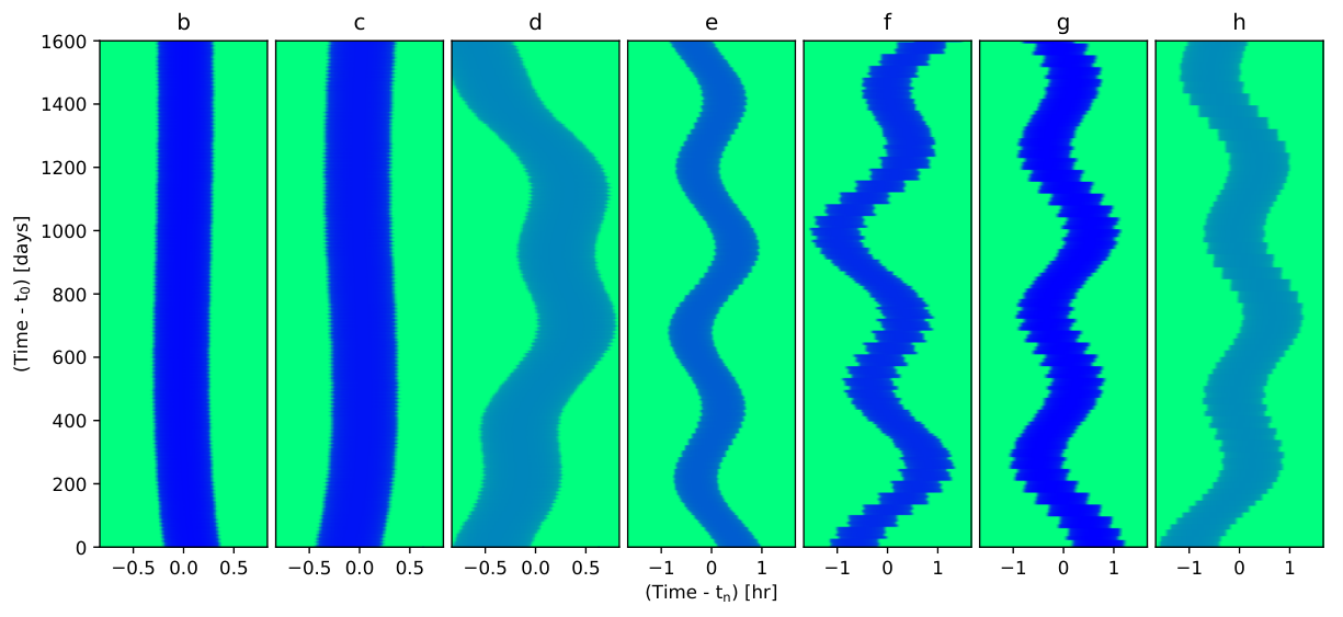
Table 3 shows the radius-ratios from Delrez et al. 2018a alongside those from the present analysis. The precision of the measurements did not improve significantly, while the radius-ratios shifted by 1-2. Figure 8 shows the posterior probability distribution of impact parameters in units of the stellar radius, , derived from the photodynamical model. Figure 9 shows the probability distribution of stellar density. The density correlates with the impact parameters of each planet, reaching a tail of lower values for higher impact parameters of each planet. The tail of the density probability distribution has an approximately exponential scaling with the density below the peak, and cuts off as a normal distribution above. In table 5 we report the median and 68.3% confidence interval of the stellar density. The inferred density is both slightly larger and more precise than prior analyses (Delrez et al. 2018a), which we discuss below.
Combining the measured density with the measured orbital periods of the planets, we derive the semi-major axis of each planet in units of the stellar radius,
| (11) |
With the measured impact parameters, we compute the inclinations of the planets from (Winn 2010)
| (12) |
where we have neglected the eccentricity in this formula due to the extremely small values of the eccentricities of the planets from the transit-timing analysis (cf Table 2). The resulting inclination posterior distribution is displayed in Figure 10. Although the inclination is derived from the impact parameters, which we constrain to be positive, in practice the photodynamical model cannot distinguish between inclinations of and (Fig. 10), and so we created a histogram of these two options with equal probability.
V.2 Mutual inclinations and stellar density
The outer four planets, through , have inclinations which are more precisely determined, and, remarkably, their peak probabilities are aligned very closely, to less than 0.1∘, save for the degeneracy of vs. . The inner three planets have poorer constraints upon their inclinations due to the larger uncertainty of their impact parameters (as seen in Figure 8). Yet, their inclination posteriors have significant overlap with the outer four planets.
As just mentioned, since each inclination may only be inferred relative to the center of the star, the derived distribution is reflected through . However, if some of the planets orbited above and some below the plane of disk of the star, it would be very improbable for the outer four planets to show such a precise alignment. We conclude that it may be likely that all of the planets transit the same hemisphere of the star as shown in Luger et al. 2017a: the planets’ 3D orbital inclinations are likely precisely aligned. This also implies that their longitudes of ascending node are likely aligned as well, and so in principle we can place a prior on the scatter of the mutual inclinations of the planets. We have re-run a photodynamic Markov chain with an inclination prior such that the planets’ inclinations are drawn from a Gaussian about their mean value, with a standard deviation of which is allowed to freely vary in the chain. We find a very tightly aligned distribution of inclinations under this assumption, shown in Figure 11. We also find that very small values of are preferred, with . If the outer and inner planets are in fact derived from a common inclination distribution, this implies that the TRAPPIST-1 planetary orbits are extremely flat, even flatter than the Galilean moons which have a dispersion in inclination of .
The inclination prior also enables a more precise and symmetric estimate of the density of the star, . Why is this? Well, the inclination prior tightens the distribution of the impact parameters of planets b and c (as can be seen by comparing Figures 10 and 11). These inner two planets have deep and frequent transits and the sharpest ingress and egress, and hence they provide the tightest constraint upon the density of the star of all seven planets (Ducrot et al. 2020). Thus, given that the inclination prior tightens the distributions of inclinations of these two planets, the stellar density posterior is correspondingly tighter, and the low stellar density tail of the posterior is eliminated (see Figure 9). Despite this tighter constraint upon the stellar density, we decide to forego its use in computing the densities of the planets given the assumptions inherent in the inclination prior.
| Parameter: | |||||||
|---|---|---|---|---|---|---|---|
| Value: | |||||||
| Parameter: | [g/cm3] | ||||||
| Value: | |||||||
| Planet: | b | c | d | e | f | g | h |
| Depth [%] | |||||||
| T [min] | |||||||
| [min] | |||||||
| [∘] |
The coplanarity of the planets may be used to constrain the presence of a more distant, inclined planet given the scatter in their mutual inclinations induced by gravitational perturbations (Jontof-Hutter et al. 2018). Such an analysis should be carried out, but we leave this to future work.
VI Planet densities and mass-radius relation
With the completion of the transit-timing analysis and photodynamic analysis, we are now ready to revisit the mass-radius relation of the TRAPPIST-1 planets.
The only component missing is a constraint upon the mass of the host star. We use the recent analysis by Mann et al. 2019, who have constructed a sample of nearby M-dwarf binaries to calibrate the mass-luminosity () relation of M-dwarfs down to a mass of 0.075 .1111 11 Note that “M” is being used in three ways here: spectral category (M-dwarf), stellar mass (), and absolute magnitude in the band, . Given the precise parallax measurement available for TRAPPIST-1 thanks to GAIA (Lindegren et al. 2018), the relation yields an estimated mass of .
To derive the masses of the planets, we draw planet-to-star mass ratios from the posterior distribution of the transit-timing analysis (§IV), which we multiply by the mass of the star drawn from a normal distribution with . We then draw the planet-to-star radius ratios and stellar density from the posterior distribution from the photodynamic analysis (§V). With the same mass draw, we compute the stellar radius as
| (13) |
which we multiply by each of the radius ratios drawn from the same sample to obtain the planet radii. We carry this out for a large number of samples to derive the probability distribution of the masses and radii of the entire posterior probability sample of the planets.
The probability distribution for the masses and radii of the seven planets are shown in Figure 12. The maximum likelihood values and the posterior distributions (for 1- and 2- confidence) are both plotted in this figure. We postpone to §IX a detailed analysis of the densities and resulting constraints on the bulk compositions of the planets.
In addition to masses and radii, we also derive other planetary properties, given in Table 6. Each of the planets has a density intermediate between Mars ( = 3.9335 g/cm3 = 0.713 ) and Earth ( g/cm3). The surface gravities span a range from 57% of Earth (planet h) to 110% of Earth (planet b).

| Planet: | b | c | d | e | f | g | h |
|---|---|---|---|---|---|---|---|
| [] | |||||||
| [] | |||||||
| [] | |||||||
| [] | |||||||
| [] | |||||||
| [] | |||||||
| [] | |||||||
| [ cm] | |||||||
| [ g] | |||||||
| [ g cm-3] | |||||||
| [ m s-2] | |||||||
| [] | |||||||
| [] | |||||||
| [ cm] |
VII Stellar parameters
A byproduct of our analysis is a revision of the properties of the host star. The empirically-based mass estimate for the star based on Mann et al. 2019 is consistent with the mass derived by Van Grootel et al. 2018, who first proposed that the mass of the TRAPPIST-1 star is based upon stellar evolution models and a ground-based parallax measurement. Ducrot et al. 2020 find a luminosity for the star of , which, when compared with stellar evolution models, yields a mass of , which is also consistent with the Mann et al. 2019 value. Burgasser & Mamajek 2017 found an older age for the host star, Gyr, which implies an inflated radius for the star compared with evolutionary models.
| Parameter | Value | Ref |
|---|---|---|
| [] | Mann et al. 2019 | |
| [] | This paper | |
| [] | Ducrot et al. 2020 | |
| [K] | This paper | |
| This paper |
Our analysis differs slightly from our prior Spitzer analyses (Delrez et al. 2018a; Ducrot et al. 2020) in that we do not place a prior upon the quadratic limb-darkening coefficients of the TRAPPIST-1 host star. This is motivated by the fact that late M dwarf atmospheres are very complex to model and have yet to match observed spectra precisely (Allard et al. 2011; Allard et al. 2012; Juncher et al. 2017), and thus it is possible that limb-darkening predictions may not be reliable. We investigated using a higher-order quartic limb-darkening law, and found that this was disfavored by the Bayesian Information Criterion, and that the best-fit model differed negligibly in the model parameters. We also simulated more realistic limb-darkening models based on 3D stellar atmospheres (Claret 2018) and found that a quadratic law was sufficient to recover the correct model parameters with negligible systematic errors.
The TRAPPIST-1 system has the advantage that the planets sample different chords of the stellar disk (Figure 8; also see Delrez et al. 2018a), and given the large number of transiting planets, we are afforded multiple constraints upon the stellar limb-darkening parameters. Figure 13 shows our posterior constraints upon the limb-darkening parameters of the star based on our photodynamical model, which are reported in Table 5.
.
Based on the updated stellar density, we have updated the physical parameters of the star. We adopt the luminosity from Ducrot et al. 2020 and the mass from Mann et al. 2019 given the complete and careful analysis from both of those papers. With our updated constraint upon the density of the star, we re-derive the other parameters of the star, which are summarized in Table 7. In this table the stellar effective temperature was computed from the stellar luminosity and radius, with errors computed via Monte Carlo.
VIII Search for an eighth planet
With the detection of multiple transits of the six inner planets in TRAPPIST-1, and a single transit of planet h, a clue as to the orbital period of planet h was the series of GLRs found between adjacent triplets of planets (Papaloizou 2014). This relation was then used to predict candidate periods of planet h, based on different integer pairs for its commensurability with planets f and g, and a search through the prior data eliminated all but one possibility at 18.766 days. A subsequent observation of the TRAPPIST-1 system with the K2 spacecraft revealed four more transits of planet h occurring at precisely the period that was predicted (Luger et al. 2017b). The existence of the GLRs amongst the known seven planets has been used to forecast the possible existence of an eighth planet interior (Pletser & Basano 2017) and exterior (Kipping 2018) to the seven known transiting planets. There is yet to be a definitive detection of an eighth transiting planet based upon the currently available data (Ducrot et al. 2020).
It may be possible to detect an exterior eighth planet via transit-timing variations induced on the inner seven planets. Planet h should experience the strongest perturbations by an exterior eighth planet due to the fact that transit-timing variations are a very strong function of the proximity of planets to one another, and also to resonance. Table 8 shows predictions for the period of planet “i", , assuming a GLR configuration with planets g and h given by
| (14) |
for a range of , which is the same range of integers for the GLRs amongst the inner seven planets. Interestingly these cases are all close to a period ratio with planet h, and thus should strongly perturb planet h due to forcing at this frequency.
| p | q | [day] | j | |
|---|---|---|---|---|
| 1 | 1 | 39.029 | 2.08 | 1 |
| 1 | 2 | 25.347 | 1.35 | 3 |
| 1 | 3 | 22.695 | 1.21 | 4 |
| 2 | 3 | 28.701 | 1.53 | 2 |
We carried out a transit-timing search for an eighth planet by placing planets with mass ratios between at these four trial orbital periods in a coplanar configuration with the other seven planets drawn from a random orbital phase at the initial time, and with eccentricity vector elements drawn from a random normal of width 0.005. We placed a Gaussian prior on the eccentricity vector elements of the eighth planet with a standard deviation of to avoid unstable configurations. We then optimized the likelihood with the eight-planet model, carrying out 11,200 optimizations on 112 CPUs with 100 optimizations per CPU, lasting seven days each for about 20,000 CPU hours.
We then carried out a search for evidence of perturbations by planet i by determining if the optimized likelihood of the transiting planets was improved by adding an eighth planet to the transit timing model, using the Bayesian Information Criterion (BIC) to penalize the additional degrees of freedom of the eight-planet model (Wit et al. 2012). We searched for a change to BIC for the eight-planet model over the seven-planet model with a difference of better than . Given that the inner seven planets show orbital eccentricities with values , we only considered an eighth planet candidate plausible if it shows an eccentricity less than this cutoff.
In all 11,200 trial optimization cases we found that only two of the eight-planet models did exceed the BIC criterion, but both significantly exceed an eccentricity of 0.01. Figure 14 shows the change in BIC versus orbital period and mass for planet “i", assuming a mass of the star of . These two cases with do not appear to be plausible planet candidates: they only just exceed the BIC criterion; they both have large eccentricities; and they are not in close proximity to a GLR with planets g and h (even though the initial parameters of the optimization were started near a GLR).
We also carried out a search for an eighth planet interior to planet b, and found even smaller improvements in the log likelihood than in the exterior case.
We have not carried out an exhaustive search for eight-planet models at other orbital periods due to the significant volume of parameter space to search. However, it is still possible that an exterior eighth planet is perturbing planet h, and may modify its transit times to a point that affects the posterior masses we infer from our seven planet model. In principle one could include the effect of an eighth planet on the mass inference by adding it to the Markov chain modeling; in practice this would be a challenging model to sample due to the multi-modal nature of the parameter space. We defer such analysis to future work.
IX Interior compositions
In this section we present theoretical interpretation of the planets’ interior properties based upon the mass-radius relation we inferred in §VI. As there is significant degeneracy in the possible interior compositions, we present a menu of different possibilities in §IX.2. However, we start with an approach which is less dependent upon the assumption of interior composition, which we term the “normalized density."
IX.1 Initial analysis of planet densities across the system
The probability distribution for the masses and radii of the seven planets are shown in Figure 12 alongside several theoretical mass-radius relationships added for comparison. We have added three rocky mass-radius relationships with different bulk Fe/Mg compositions: (1) molar Fe/Mg as suggested by Unterborn et al. 2018 to represent the rocky interior of all TRAPPIST-1 planets with a 1 range of Fe/Mg ratios consistent with local stellar abundances; (2) the Sun-like value of molar Fe/Mg (Lodders et al. 2009); and (3) a core-free model with Earth-like refractory ratios, but in which all of the iron is oxidized in the mantle (Elkins-Tanton & Seager 2008). Rocky interiors are calculated similar to the models of Dorn et al. (2016) with two adaptations: we are using the equation of state of Hakim et al. 2018 for pure iron and Sotin et al. 2007 for silicates. We have also added the theoretical mass-radius relationships for planets endowed with a water layer, both for planets which are irradiated less (black line; water) and more (umber lines; steam) than the runaway greenhouse irradiation threshold (Turbet et al. 2020).
The comparison of measured masses and radii with theoretical mass-radius relationships reveals several striking results. First, all seven TRAPPIST-1 planets appear to be consistent with a line of interior isocomposition at the level. There are multiple theoretical mass-radius curves that overlap with all seven planets’ mass-radius probability distributions (Fig. 12), which may be a good indication that the composition varies little from planet to planet. Secondly, all of the TRAPPIST-1 planets have lower uncompressed densities than Solar System terrestrial planets. This likely means that the TRAPPIST-1 planets either have a lighter interior (e.g. lower iron content) or are enriched with volatiles (e.g. water).
We next searched for variations of density across the planets. For this, we took each planetary density calculated from samples and divided by the density of the closest pair of mass and radius of a fully differentiated 20 wt% iron, 80 wt% silicate (MgSiO3) interior planet with no surface layers, which is less iron rich than Earth. A planet with a normalized density of 1 has exactly the same density as the reference model, while a normalized density () is denser (lighter), than the reference model, respectively. Fig. 15 shows the resulting histograms of the posterior probability of the normalized TRAPPIST-1 planet densities. We then plot in Fig. 16 the normalized densities (along with their 1 uncertainty) as a function of the orbital periods of the planets. The normalized planet density appears very uniform across the seven planets, with perhaps a slight decrease with the increase of the orbital period (or the distance to the host star). We fit a line to the normalized density, , versus orbital period, , for posterior samples, and found a relation of where the coefficients are the 68.3% confidence interval. There is only weak evidence for a declining trend of normalized density with orbital period: 88% of the fits to the posterior samples have slopes with a negative value, while 12% of the slopes fit have a positive value. If in the future more precise data strengthen this trend, then this may indicate that either (i) the outer planets are depleted in heavy elements (e.g. iron) compared to the inner ones, or (ii) the outer planets are enriched in volatiles (e.g. water) compared to the inner ones. However, based on the current data we suggest that the planets’ compositions could be rather uniform in nature.
The interpretation of these observations in terms of internal compositions is discussed in more detail next.
IX.2 Range of possible interior compositions and volatile contents
In this subsection, we discuss a range of possible compositions of the planets based on their measured densities, starting with a volatile-poor model in which the densities are fit by varying the core-mass fraction (§IX.2.1), and followed by an analysis in which the solid planets are taken to have an Earth-like composition, to which is added a water fraction needed to create the observed densities (§IX.2.2). Alternatively, the planets might be explained with an enhanced oxygen content by which all of the iron is oxidized making the planets core-free (§IX.2.3).
IX.2.1 Core Mass Fraction
If we assume that the planets’ atmospheres contribute a negligible amount to their total radius, and that the planets are fully differentiated, composed of rocky mantles (MgSiO3) and iron cores only, then the densities may be used to constrain the portion of the planets’ mass which is contained within their cores.
We evaluated the core mass fractions (CMF) of the TRAPPIST-1 planets as follows. For each mass/radius pair in our posterior distribution we have estimated the core-mass fraction by linearly interpolating between pre-calculated mass-radius relationships with our employed interior model. We arbitrarily set each mass/radius pair lighter than a pure silicate (MgSiO3) planet to a CMF of 0. Alternatively, we repeated the same procedure but discarding all CMF values lower or equal to 0. However, we found that the estimate of the core mass fraction is only marginally changed (and only for planets g and h).
Our core mass fraction estimates are provided in Fig 17 and Table 9. Estimates range from wt% for planet g up to wt% for planet c, which, despite the different central values, have considerable overlapping probability distributions. Fig 17 shows that within the uncertainties, the CMF/Iron fraction of the planets are very consistent with one another, with the mean of all planets of wt% (taking into account the correlations between the planets’ core-mass fractions).
There may be a slight trend of the inferred CMF, which decreases with increasing orbital period. The trend is qualitatively similar to that reported on the normalized density (see Fig. 16), with similarly weak support: only 88% of the linear fits to the posterior CMF values have a slope with orbital period which is negative, whilst 12% are positive.
| Planet: | b | c | d | e | f | g | h | Avg b-h |
|---|---|---|---|---|---|---|---|---|
| CMF [wt%] | ||||||||
| Fe/Mg molar ratio | ||||||||
| H2O [wt %] for: | ||||||||
| CMF=18% | ||||||||
| CMF=25% | ||||||||
| CMF=32.5% | ||||||||
| CMF=50% |
IX.2.2 Surface water content

The observed (weak) variation in the planet densities among all seven planets may instead be due to their differing volatile (e.g. water) inventories.
If we assume a rocky Earth-like interior (CMF=32.5%, fully-differentiated) and only allow an additional condensed1212 12 Note that it is likely unwarranted to assume condensed surface water for the inner three planets given their location within the runaway greenhouse zone (Turbet et al. 2020). water layer to contribute to the total radius, we can estimate the water mass fractions of the seven planets (b: wt%, c: wt%, d: wt%, e: wt%, f: wt%, g: wt%, h: wt%). The lower densities of planets d, f, g, and h can allow for two to three times as much water than for planets b, c, and e. For this simple estimate we assumed a water layer with a surface temperature of 300 K at 1 bar.
Actual surface conditions and assumed iron content can, however, lead to much larger differences in the estimated water budgets between the inner three and outer four planets. This stems from the fact that the inner three planets are more irradiated than the runaway greenhouse irradiation limit (Kopparapu et al. 2013; Wolf 2017; Turbet et al. 2018) for which all water is vaporized, forming a thick H2O-dominated steam atmosphere. Taking into account the expectation that water should be vaporized for the three inner TRAPPIST-1 planets (Turbet et al. 2019; Turbet et al. 2020), their water mass fractions drop drastically to less than wt%, i.e. more than several times lower than the water ocean mass fraction of the Earth.
Figure 18 shows the expected water mass fractions for each of the TRAPPIST-1 planets, and for four distinct interior compositions (18, 25, 32.5 and 50 wt% iron content). It shows that the same qualitative trend of water versus orbital period is relatively robust across a large range of assumptions on the interior composition thanks to the transition from runaway greenhouse for planets b-d to surface liquid water for planets e-h.
Higher estimated water budgets for the outer three or four planets could be a clue that they formed beyond the water condensation line at 0.025 AU (Unterborn et al. 2018). This could also be due to the significant differences in water loss (through atmospheric escape) arising from variations of irradiation and gravity among the TRAPPIST-1 planets (Lissauer 2007; Bolmont et al. 2017; Bourrier et al. 2017). However, again, we caution again that trends in the planetary volatile content are only weakly supported by the current data.
IX.2.3 Core-free planets
Given that the data may be consistent with an iso-composition mass-radius relation, we next consider another intriguing possibility: that the interiors of the planets are fully oxidized. If, instead of forming a core, all of the iron is oxidized and remains in the mantle, the size of a planet may increase by a few percent (Elkins-Tanton & Seager 2008). This turns out to be about the amount of radius inflation necessary to match the TRAPPIST-1 planets when compared with our Solar system planets.
If we assume that the refractory ratios match a Solar composition, and that all seven planets lack an atmosphere, then it turns out that all seven planets are consistent with a core-free, oxidized composition (Fig. 12; red line). For this model the bulk mass abundance ratios for Fe/Si/Mg/O are 29.2/17.3/15.3/38.2 wt% with a magnesium number of 0.55 (Mg/(Mg+Fe)) mol fraction; this model has a significant increase in oxygen compared to the bulk Earth with 29.7 wt% (McDonough 2014). Such a scenario would likely require formation of the planets at large distances from the star in a highly oxidizing environment (Elkins-Tanton & Seager 2008) and a lower devolatization temperature intermediate between that of Earth and chondrites (Wang et al. 2019). Hence, although this hypothesis efficiently explains the TRAPPIST-1 data, it remains to be seen whether a geochemical model can be constructed which results in high oxidation of iron throughout the processes of planet formation and evolution (Kite et al. 2020).
X Discussion
Here we discuss some of the implications of the results in the foregoing sections.
X.1 Timing uncertainties
As reported in §III, the transit timing measurements we have made show an excess of outliers with respect to the measurement uncertainties of each transit. We were unable to identify a culprit (or culprits) for these discrepancies, but wish to speculate on what may be the origin of these outliers. The cumulative distribution of these outliers (Fig. 1) indicates that about 10% of transits are affected at some level. It is also interesting to note that the core of the distribution has a slightly smaller width of about 87% of the measurement errors, indicating that for about 90% of the transits, the uncertainties may be overestimated. This may be a consequence of inflating the uncertainties to account for correlated noise rather than modeling the data with, for example, a Gaussian process; further re-analysis of the data will be needed to check this hypothesis.
Could the timing outliers be due to stellar flares? In Vida et al. 2017 and Ducrot et al. 2020, the frequency distribution of stellar flares is shown to be rising towards smaller flare energies. This could mean that the more frequent, but lower energy flares, occur at a level that is swamped by the photon noise, and thus not visible to an observer. We used the spectrum and energy calibration of Spitzer flares measured by Ducrot et al. 2020 to extrapolate the frequency of lower energy flares (which are not detected in Spitzer due to photon noise). As an example, for planet h the transit time can be affected by a flare which occurs at ingress or egress (duration min). We estimate that a flare of energy erg could cause a 1.5 timing outlier if it occurs during ingress or egress. This has a probability of only % to occur during the 10 minutes of ingress or egress, and thus cannot be responsible for 10% of outliers for planet h. We carried out a similar estimate for the other planets, and we conclude that low-level flaring activity cannot be the cause of the timing outliers.
Other possible causes of the timing outliers are correlated stellar variability, star spot crossings, or instrumental systematics. We don’t yet have an estimate of the magnitudes of these effects, and so cannot reach a conclusion about where the origin of the timing outliers lies.
X.2 Possible systematic errors
In this section we consider possible factors which might affect our inference of the densities of the planets. Simulated planetary densities predict core-mass-fractions which are similar to Earth, with a very small scatter (Scora et al. 2020). Hence, the fact that the TRAPPIST-1 planets have inferred planetary densities which are less than this could be due to systematic uncertainties which are not captured by our modeling.
The transit depths determine the planet-to-star radius ratios, but these measurements are affected by the non-uniform surface brightness of the star. Fortunately the multiple impact parameters of the planets yield a constraint upon the infrared limb-darkening, which is fairly weak compared with optical bands. However, star-spots can also affect the inferred transit depths (Czesla et al. 2009; Oshagh et al. 2013; Oshagh et al. 2014; McCullough et al. 2014; Rackham et al. 2018; Kipping 2012). If spots are present on an active latitude which is not on the same hemisphere as the planetary transit chords, this can cause all of the planet radii to be mis-inferred by a similar factor.
TRAPPIST-1 may have complex surface inhomogeneities, including regions brighter or darker than the mean photosphere (Morris et al. 2018; Zhang et al. 2018; Wakeford et al. 2019). It is possible that bright or dark regions could bias the apparent transit depths towards larger or smaller measurements, depending on which type of inhomogeneity dominates. Time-variable contamination should average out with many observations, while time-steady inhomogeneity will not, such as active latitudes, polar spots, or even hemispheric asymmetry (Yadav et al. 2015; Brown et al. 2020). We modeled the transit-transmission in the K2, SPECULOOS, LT, near-infrared, and Spitzer bands from Ducrot et al. 2020 for all seven planets using the contamination formula from Rackham et al. 2018 with a time-steady, three-temperature model with the temperatures of the three components ranging from 2000-2980 K and the covering fraction varying from 0 to 1. The mean effective temperature is constrained by our stellar model parameters (Table 7). We assumed that all seven planets transit the region with the larger covering fraction, and that their transit depths are achromatic. We ran a Markov chain fit to the transmission spectra, interpolating the fluxes in the bands between the effective temperature grid points which were spaced by 20 K; we find that the posterior parameters with maximum likelihood are temperatures of K with covering fractions of %. We then computed the expected impact on the transit depths in the two IRAC channels. The constraints are tight: we find that the observed radii should only change by a factor of in Channel 1 and in Channel 2 (these are the ratios of the observed radii to the actual radii). These factors are consistent with unity at better than , and have uncertainties which are comparable to or smaller than the uncertainties on the absolute planetary radii. We conclude that this form of self-contamination does not greatly influence our results, but should lead to caution in the interpretation. This constraint is much stronger than the analysis of Morris et al. 2018.
Our mass precisions are predicated on a complete model of the dynamics of the system. We neglect tides and general relativity, which are too small in amplitude to affect our results at the current survey duration and timing precision (Bolmont et al. 2020). Should an eighth planet be lurking at longer orbital periods, which has yet to reveal itself via significant transit-timing variations or transits, this may modify our timing solution and shift the masses slightly. In our timing search for an additional planet, however, we found that such a planet might only cause shifts at the level. This possibility begs for caution in interpreting the potential variation of iron fraction with orbital period: should an eighth planet be present beyond planet h, its timing impact would likely affect the masses of the exterior planets more significantly than the interior planets. Drawing stronger conclusions about the variation of planet iron/core mass fractions will likely require longer-term monitoring, especially of planet h, and/or higher precision timing measurements such as are expected with JWST, to place tighter constraints on an eighth planet.
X.3 Planet masses and radii in context
In our current analysis of the transit-timing data for TRAPPIST-1, we have found larger mass ratios for all planets save planet e compared with our most recent analysis in Grimm et al. 2018. Even though most of the planets have shifted by 1 or more, this does not indicate that the prior analysis was in error. In fact, the masses of all of the planets are strongly correlated, and thus when one planet shifts in the transit-timing solution, they all shift. With the more extensive dataset analyzed here, we provide a better constraint over the transit-timing timescale, and can also better account for outliers thanks to some redundancy in our measurements. Given the high precision of the Spitzer timing measurements, we expect that our current analysis may remain the most reliable constraint upon the masses of the planets until the transit times can be measured with JWST.
In Figure 19 we compare our measurements for the seven TRAPPIST-1 planets with our Solar System planets and with exoplanets with radii and masses measured to retrieved from the NexSci database on 26 Feb 2020 (Akeson et al. 2013; Christiansen 2018), as well as planet parameters reported in Dai et al. 2019 and Kepler-93b from Dressing et al. 2015.1313 13 Note: we corrected Kepler-105b with the GAIA DR2 revised radius of the host star (Berger et al. 2018; Fulton & Petigura 2018). The uncertainties on the other planets’ masses are the best available to date from radial-velocity measurements, and yet they are much larger than the uncertainties for the TRAPPIST-1 planets, whether considered in a relative or absolute sense. The larger uncertainties of the RV planets makes the core-mass fractions difficult to constrain for these more massive planets - core-free and cored models are consistent with most of these planets’ parameters at the 1 level (Fig. 19). Nevertheless, it is notable that the rocky planets for which we currently have data seem to be similar in composition to the Earth (Dressing et al. 2015); however, the actual range of bulk rock compositions of rocky exoplanets relative to their host stars is currently debated. This also appears consistent with the observation that the evaporation valley requires rocky planets and their gaseous brethren to have a composition which is a mix of silicates and iron (Owen & Wu 2017).
X.4 Comparison with radial velocities
Given the measurements of the masses we have made with transit-timing, this brings up the question: what radial-velocity uncertainties would be required to make mass measurements of similar precision?
The precision of the mass measurements may be placed in context by comparing with current radial-velocity capabilities. The predicted semi-amplitudes for the seven planets are given in Table 10. The predicted radial-velocity variation of the star induced by the TRAPPIST-1 planets is plotted in Figure 20, also based upon our mass measurements from transit timing. The sums of the semi-amplitudes of the planets equals m/sec, which is close to the peak amplitude when the planets are all orbiting on the same side of the star (near 218 days in the plotted figure). How does this compare with current RV measurements?
Recently Hirano et al. 2020 were able to make high precision measurements of the radial velocity (RV) of the TRAPPIST-1 host star, achieving a constraint on the linear variation of the star to a precision of 2.5 m/sec which they ascribe to stellar variability. To compare this with our transit-timing results, the semi-amplitude precision which would be needed to achieve the same mass error bars that we have achieved with transit-timing ranges from 2.4-19 cm/sec, up to 100 times more precise than the radial-velocity measurements. Future observations may be able to achieve higher precision radial velocity measurements of TRAPPIST-1, but will continue to contend with stellar variability (Klein & Donati 2019).
Were these planets orbiting a Sun-like star, the semi-amplitude RV error would need to be even smaller to achieve the same mass precision we have achieved with transit timing. Table 10 lists what semi-amplitudes precisions would be required if each one of these planets was placed around a Solar twin at one astronomical unit. The required precision ranges from 1-6 millimeters/second. This is nearly two orders of magnitude more precise than the highest precision RV measurements for short-period exoplanets reported to date, such as Tau Ceti g, which has a reported RV semi-amplitude precision of 11 cm/sec (Feng et al. 2017). We conclude that the mass precisions of Earth-sized, Earth-insolation planets based on radial velocity must be improved by two orders of magnitude to match our TTV precision for the TRAPPIST-1 system.
| Planet | b | c | d | e | f | g | h |
|---|---|---|---|---|---|---|---|
| [cm/sec] | 382.0 | 310.7 | 77.6 | 120.7 | 158.1 | 182.2 | 39.1 |
| RV equivalent precision for TRAPPIST-1 host [cm/sec] | 19 | 13 | 2.5 | 3.8 | 4.7 | 5.2 | 2.4 |
| RV equivalent precision for 1 host at 1 AU [cm/sec] | 0.62 | 0.50 | 0.11 | 0.20 | 0.28 | 0.34 | 0.18 |
X.5 Planetary dynamics
In this section we discuss some of the dynamical aspects of the planetary system: the eccentricities, the longitudes of periastron, and the GLR angles.
X.5.1 Eccentricities
The posterior distribution of the initial eccentricities of the planets is shown in Figure 21. In prior analyses of the transit-timing variations of the TRAPPIST-1 system we found that the inner two planets, b and c, had significant eccentricities (Grimm et al. 2018). In contrast, with the current analysis we find that the eccentricity probability distributions of these two planets are significant near zero eccentricity. This is consistent with N-body models which include tidal damping of the orbits, which predict that the planets b and c should have low eccentricities, (Luger et al. 2017b; Turbet et al. 2018). The other planets are all consistent with the predictions of the tidal evolution model (Luger et al. 2017b).
Figure 22 shows the posterior probability distribution for the eccentricity vectors of each planet. The only two planets consistent with zero eccentricity at 1 confidence are planets b and c (blue and orange contours). The other five planets have non-zero eccentricities.
Now, the eccentricity vectors plotted in Figure 22 show the values at the initial time. However, over time, the eccentricity vector of each planet can be decomposed into two components: the mean eccentricity vector (over some timescale) and the variable component (which is time variable, with multiple oscillation timescales driven by the mutual planetary perturbations). Figure 23 shows the eccentricity over a single oscillation for all seven planets. The outer five planets are close to first-order resonances with adjacent planets, and the super-period for each of these planets is close to days thanks to the near-GLR commensurability for all triplets of planets. This leads to a nearly circular oscillation over this timescale due to circulation of the first-order resonances driving oscillations in the eccentricity vectors of each of these planets. The inner two planets are close to second and third order resonances with adjacent planets (b and c are close to 8:5, which is third order, while c and d are close to 5:3, which is second order). Since the strength of these interactions scales as a higher power of eccentricity, these planets show much smaller variation in the time-variable components of their eccentricity vectors. Since planets b and c are close to a third order resonance, their eccentricity vectors show a three-fold symmetry. On longer timescales these patterns precess, filling a circular pattern over time. The time-variable eccentricity vector patterns are very similar over the range of posterior values, indicating that it is primarily this component which is constrained by the transit timing variations of the planets.
The total eccentricity vectors show a wider range of behavior, thanks to a wider variation of the mean eccentricity, as shown in Figure 24. It is clear from this figure that each planet executes an eccentricity-vector oscillation about a mean value (which was subtracted off for figure 23). Unfortunately the mean eccentricity is less constrained by the transit-timing variations (Linial et al. 2018), and so there is a much wider range of eccentricity vectors which is allowed which manifests as strong correlations amongst the eccentricity vectors of pairs of planets (Figure 29).
X.5.2 Laplace angles
A remarkable property of the TRAPPIST-1 system is the near-commensurability of adjacent triplets of planets (Luger et al. 2017b), akin to Laplace resonances, with GLR angles given by
| (15) |
where is the mean longitude of the th planet, and and are small integers. In the case of an isolated triplet of planets, a stable configuration takes on , but when planets are captured into a series of GLR commensurabilities, their mutual torques displace the stable configuration (Delisle 2017).
Long-term dynamical simulations show that these GLR angles can take on stable values for extended durations, and sometimes can quickly jump in value, flipping symmetrically about 180 degrees (Mah 2018; Brasser et al. 2019), resulting in two possible angles for each triplet of stars, and . Based on the prior measured planet-to-star mass ratios, Mah 2018 predicted the value of the three-body resonance angles resulting from the values at the end of the simulation.
In Figure 25 we show the GLR angles for the following triples:
| (16) | |||||
| (17) | |||||
| (18) | |||||
| (19) | |||||
| (20) |
Differences between the predicted and observed angles agree within 0.5-10 degrees, where the predicted values for are taken from Mah 2018, but allowing and to be flipped about 180 degrees. It is possible with the updated mass-ratios from our analysis that the predictions will be more accurate, which awaits further simulation.
X.5.3 Long-term stability
Prior studies of the TRAPPIST-1 system by Tamayo et al. 2017 found long-lived configurations for systems which had formed via migration. Quarles et al. 2017 examined the stability of the TRAPPIST-1 system, refining the large uncertainties from prior measurement (Gillon et al. 2017) to further constrain the masses of the system. Given the much tighter constraints we have placed upon the masses of the planets and the orbital eccentricities, here we re-examine the long-term stability of our posterior distribution.
We have used the GPU N-body integrator GENGA (Grimm & Stadel 2014) to carry out long-term simulations of a set of posterior samples from the timing analysis. These simulations were carried out for years, which corresponds to 2.4 billion orbital periods of planet b, and 195 million orbital periods of planet h. We used a time step of 0.06 days, which gives a total number of integration steps. We find that 100% of these posterior samples are stable over this entire timescale. To check the stability of the samples, we analyzed the evolution of the semi-major axis, , and eccentricity, , of all samples and planets. We compared the average values over the first Myr and the last Myr. Table 11 gives the average over all samples, and the maximum differences between the first and the last Myr. In all cases the variations are small, . These results suggest that the simulations could be stable even on a much longer time scale. In addition, we have carried out long-term (50 Myr) integrations with tidal damping for two posterior samples, one with low and one with high values of the eccentricity of planet b. Using a range of values of tidal damping (from 1/10 to 100 times Earth’s), we find in all cases that the system remained stable (Bolmont et al. 2020, using Posidonius;).
More interesting is the evolution of the five GLR resonant angles, shown in Figure 26. In order to describe the evolution of the GLR angles, we define three categories:
- •
Category I: remaining in GLR for 10 Myr, with a maximum difference to the initial value of less than
- •
Category II: remaining in GLR for 10 Myr, with a maximum difference to the initial value of more than . In this category, the GLR angles can jump between different states.
- •
Category III: not remaining in GLR for 10Myr.
The threshold of is chosen arbitrarily, but is found to be practical to distinguish simulations where the GLR angles jump between different states (Category II), or remain in the same state (Category I). Figure 26 shows the three different categories in different colors, as well as a histogram of all 10,000 simulations over 10 Myr for all five GLR angles. The exact number of simulations in the three categories are given in Table 12. The GLR angles from Planets b,c and d as well as Planets d,e,f show a unique resonant state. Planets c,d,e and Planets e,f,g have a dominant state and a subdominant state, while Planets f,g,h have a dominant state and two symmetric subdominant states. Our new samples show a better conservation of the GLR angles than was found in Grimm et al. 2018, where the longest resonance time was found to be 2 Myr.

| planet | |||||
|---|---|---|---|---|---|
| b | -6.52e-09 | 1.73e-04 | 7.12e-07 | 0.0020 | |
| c | -1.44e-08 | 1.62e-04 | 2.51e-06 | 0.0018 | |
| d | -1.06e-08 | 1.45e-05 | 4.07e-06 | 0.0009 | |
| e | 2.05e-08 | 4.44e-05 | 8.53e-06 | 0.0008 | |
| f | 2.45e-07 | 5.13e-05 | 3.00e-05 | 0.0012 | |
| g | 8.24e-08 | 5.01e-05 | 2.19e-05 | 0.0011 | |
| h | -1.23e-07 | 2.11e-04 | 3.00e-05 | 0.0035 |
| bcd | cde | def | efg | fgh | |
|---|---|---|---|---|---|
| Category I | 130 | 178 | 755 | 7943 | 6462 |
| Category II | 1571 | 874 | 7653 | 1855 | 1578 |
| Category III | 8299 | 8948 | 1592 | 202 | 1960 |
X.6 Forecasts for JWST
X.6.1 Forecast transit times
With our transit timing model we can forecast the probabilities of future transit times, and hence better help to plan transit observations with JWST. This is important for both optimizing the efficient use of the telescope, and for determining concurrent transits (i.e. two or more planets crossing the face of the star at the same time). This is especially important for transit transmission spectroscopy as the signal will be small, and hence many transits may need to be observed. With observation of initial transits with JWST the ephemerides can be refined/updated; however, our current forecasts provide the starting point for planning JWST observations.
Table 15 gives our forecast for upcoming times of transit through October, 2023 to cover the first 2 years of the JWST mission (six months after the end of Cycle 1, given the present launch date of October 2021).
X.6.2 Simulated JWST TTV analysis
Based on the measured properties of TRAPPIST-1, we have carried out a preliminary analysis forecasting future transit observations with the James Webb Space Telescope. Already there are several JWST Guaranteed Time Observation (GTO) programs which plan to observe the TRAPPIST-1 planetary system, primarily for the purposes of spectroscopic characterization (GTO programs 1177, 1201, 1279 and 1331).1414 14 For specifications of these programs, see https://www.stsci.edu/jwst/observing-programs/ approved-gto-programs. It is very likely that additional observations will be scheduled during guest observing time throughout the duration of the JWST mission as the detection of spectroscopic features requires observations of multiple transits for each of the planets (Morley et al. 2017; Barstow & Irwin 2016; Lustig-Yaeger et al. 2019; Fauchez et al. 2020). An effort to coordinate these observations amongst the exoplanet and planetary science communities is underway via the TRAPPIST-1 JWST Community Initiative (Gillon et al. 2020). All to say, long-term studies of TRAPPIST-1 for spectroscopy will also yield transit times for each transit observed, enabling a transit-timing analysis of the results.
To estimate the maximum possible precision of observations with JWST, we have simulated a five-year program in which every transit of every planet in TRAPPIST-1 is observed with NIRSPEC (Birkmann et al. 2016). The NIRSPEC instrument was chosen as its prism mode covers 0.5-5 microns, covering the peak of the SED of the star, and thus maximizing the number of photons detected, which is about two orders of magnitude per transit greater than collected by Spitzer. Although such a complete set of transits will be impossible to collect (thanks to limits due to scheduling and time-allocation), this analysis yields an estimate of the most optimistic results we might expect from JWST.
We have carried out simulations of transits of each of the planets as observed by NIRSPEC. We include realistic estimates of photon noise and correlated stellar variability based on the pattern of variations detected with the Spitzer Space Telescope, using a Gaussian Process model created with celerite (Foreman-Mackey et al. 2017). We do not include instrumental systematics under the assumption that over the timescales of ingress/egress, which are what limit the timing precision, that the noise contribution will be dominated by photon noise and stellar variations. From these simulations, we found that the posterior timing precision ranges from 0.6-1.7 second per transit, much more precise than the measurements reported in the present paper.
Next, we created a simulated set of transit-timing observations at the two windows each year when the TRAPPIST-1 system is observable with JWST (Figure 27). For each transit time, we drew the time from the distribution of uncertainties from the posteriors of the simulated transit data.
Finally, we utilized our code for transit-timing analysis to optimize a plane-parallel model with seven planets. At the maximum likelihood of the fit, we computed the Hessian to estimate the uncertainties on the model parameters. Figure 27 shows the simulated transit-timing observations with JWST. This includes about 600 transits observed with the telescope (again, the maximum possible over the nominal 5-year JWST mission). Figure 28 shows the results of the mass measurements in the simulations. We find that the masses can be recovered to better than 0.02% for planets d-h, and to 0.1% for planets b and c.
Of course, it will be impossible to arrange such a large number of transit observations of this system. But, even if the number of observations is an order of magnitude smaller, we expect that the signal-to-noise should scale with the square root of the number of measurements made, and thus the outer planets will still have mass measurements precise to the order of a part-per-thousand.
X.7 Stellar parameters
The stellar density we derive using the photodynamic model, , is in agreement with prior analyses. Most recently, Delrez et al. 2018a found a density of , twice as uncertain as our analysis. Our approach yields a density of superior precision due to several factors. The transit times in the Spitzer data are constrained by all of the measured transits in the photodynamic model so that fewer degrees of freedom are needed to fit the times (37 free parameters in the N-body model versus 447 transit times fit to each transit).
The stellar mass we take from the analysis by Mann et al. 2019, .1515 15 https://github.com/awmann/M_-M_K- This mass has a precision of 2.6%, which limits the mass precision for several of the planets. We are at the point that to improve the mass measurements of the planets we will need to improve the measurements of the star.
We used the luminosity estimate from Ducrot et al. 2020, which is slightly lower than that estimated by Gonzales et al. 2019 due to a difference in the measured bolometric flux. We are consistent with Gonzales et al. 2019 for the reported value of at 1, while our is more precise (28 K vs 42 K), is 2.5 times more precise, and our is more precise by an order of magnitude.
XI Conclusions
The Spitzer discovery of seven transiting planets orbiting the TRAPPIST-1 star by Gillon et al. 2017 promised the determination of the interior compositions of these planets via dynamical analysis. We have now analyzed the complete set of transit time measurements of the TRAPPIST-1 planets from Spitzer, augmented by additional transits from the ground, K2, and HST. Our primary conclusions are:
- 1.
We have measured the masses, radii and densities to high fractional precision, 1-8%, based on an N-body model and a photodynamical model with seven planets. This improves upon RV current precision by up to two orders of magnitude.
- 2.
The pattern of masses and radii may be consistent with a uniform planetary composition for all seven planets which have lower uncompressed densities than the Earth, Mars or Venus, with weaker evidence for a declining normalized density with orbital period (88% confidence). The planet properties may either be consistent with a core mass fraction of wt%, or an Earth-like core and mantle with a surface water content which varies from % for the inner three planets to % for the outer four, or core-free planets with highly oxidized iron in the mantle which elevates the interior light element content. These are not unique explanations.
- 3.
The planets appear to be dynamically-cold, with eccentricities less than %, and inclinations which may be coplanar to a few hundredths of a degree.
- 4.
The system is stable on long timescales, and shows a pattern of generalized Laplace resonances with angles which match predictions from migration simulations of Mah 2018.
- 5.
We provide a forecast of the future times of transit for the planets (Table 15) to help in planning observations with JWST, which may yield more precise constraints upon the planets’ masses.
- 6.
We have yet to find strong evidence for an eighth planet.
Based upon these properties, we next speculate on some possible scenarios for the formation and evolution of the system.
XI.1 Expectations for the compositions of the TRAPPIST-1 planets from formation scenarios
As mentioned, our analysis suggests that the TRAPPIST-1 planets have somewhat lower uncompressed bulk densities than Earth (see Table 6 and Fig. 12). It is possible that these lower densities result from a deficit of high-density material (e.g., less iron) relative to Earth, or an excess of low-density material (e.g., having more water), or both; in this section we speculate about formation scenarios which may be consistent with these planets’ bulk densities.
In general, planets which formed within the same proto-planetary disk are expected to have similar budgets in relative refractory elements (Bond et al. 2010; Elser et al. 2012) but can have very different volatile element budgets (Öberg & Bergin 2016). Similar relative refractory elements (Fe, Mg, Si) implies similar core mass fractions for all seven planets, assuming full differentiation. As suggested by Dorn et al. 2018, the refractory composition may best be described by studying the densest planet of the system, planet c with 22-31% CMF. Thus, with this assumption, all of the planets may likely have a 22-31% CMF but different light element mass fractions (that may increase slightly with orbital period, Fig. 19).
Is an overall CMF of 22-31% realistic for terrestrial planet interiors? This range of CMF implies lower Fe/Mg and Fe/Si values compared to Earth (and the Sun). Elemental abundances of rocky interiors are expected to be reflected in the photospheric abundance of the host star as argued by Unterborn et al. 2018 and Dorn et al. 2018. Unfortunately, measuring the photospheric abundances of this cool and active host star remains very challenging. However, Unterborn et al. 2018 estimated the stellar molar Fe/Mg number ratio to be by analysing Sun-like stars of similar metallicity to TRAPPIST-1, which may be slightly lower than the Solar value. This corresponds to a CMF of 24-35% for a fully-differentiated model. The corresponding mass-radius curve for a rocky interior of this range of Fe/Mg value is plotted in Figure 12 (gray curve and shaded region). It overlaps well with the densest planets c and b. This means that the expected range of stellar abundances supports a possible overall CMF value of 22-31%, assuming full differentiation.
Could there be a variation of Fe/Mg ratios among the planets? Rocky planet accretion should preserve the integrated iron/rock ratio. Consider a population of planetary embryos and planetesimals that accrete into a system of rocky planets. Giant collisions between growing planetary embryos can change the iron/rock ratios of individual objects by preferentially stripping the outer, rock-dominated layers from differentiated embryos (Benz et al. 1988; Marcus et al. 2010; Asphaug & Reufer 2014, e.g.). But from a system-wide perspective, it is a zero-sum game unless rock or iron is preferentially lost from all of the planets. Rock is the major component of loosely-bound impact debris and more likely to be lost either by differential aerodynamic drag (Weidenschilling 1977) or solar wind drag (Spalding & Adams 2020), and so the integrated iron/rock ratio should only increase. Hypothetical variations in Fe/Mg can otherwise be caused if large portions of planetary building blocks condense at different high temperatures ( K). During planet formation, such temperatures are only reached in a tiny region very close to the ultracool dwarf star. Consequently, both Unterborn et al. 2018 and Dorn et al. 2018 have assumed that all seven planets have similar refractory element ratios (i.e., Fe/Si, Fe/Mg). Whether rocky planets can have a wider compositional distribution than that of stars remains to be seen (Plotnykov & Valencia 2020).
Alternatively, the lower measured bulk densities of the TRAPPIST-1 planets relative to Earth-like composition might be explained by core-free interiors (Elkins-Tanton & Seager 2008) in which the oxygen content is high enough such that all iron is oxidized. If the refractory elements (Mg, Fe, Si) follow Solar abundances, a fully oxidized interior would contain about 38.2 wt% of oxygen, which lies between the value for Earth (29.7 wt%) and CI chondrites (45.9 wt%). Such an interior scenario can easily describe the observed bulk densities (red line in Fig. 12). And this may bolster the long-range migration scenario in which the planets formed in a highly oxidizing environment which enabled the iron to remain in the mantle even after migration. Based on the elemental composition, these models have an oxygen fugacity of 1616 16 Oxygen fugacity is stated relative to the Iron-Wüstite equilibrium reaction (Wüstite) such that which is more oxidized than Earth or even Mars, but is comparable to the oxidation state of small bodies, both in our solar system and accreted by white dwarfs (Doyle et al. 2019).
However, the evidence for a core-free planet may rest on knowing the refractory abundances of the TRAPPIST-1 host star, which have yet to be constrained. Alas, our interpretation of the planets’ compositions may be limited by our imprecise knowledge of the host star: its radius, its mass, its photospheric inhomogeneity, and its refractory abundances all affect our measurement and interpretation of the masses, radii, and compositions of the TRAPPIST-1 planets. In this paper our measurements of the relative planetary radii and masses have reached such a precision that the fault may now lie in the star.
XI.2 Future work
We conclude by pointing out directions for building upon the work described in this paper:
- 1.
We have yet to identify the origin of timing outliers which show an excess relative to a normal distribution. This may be addressed with higher precision measurements which may be able to identify a source of noise responsible for these outliers.
- 2.
Our analysis assumes a plane-parallel system with seven planets, and does not yet couple the dynamical and photometric analysis (our photodynamics held the dynamical model fixed). Future analysis with a fully-coupled photodynamical model with 3D orbits and more than seven planets may be valuable.
- 3.
We need more transits measured for planets d and h, in order to better measure the amplitude and phase on the transit-timing variation timescale, as well as to better constrain the presence of planets beyond h.
- 4.
The interpretation of the compositions of the planets is limited by the unknown composition of the host star. A measurement of the Mg/Fe and Fe/Si ratios would help to interpret the core and mantle compositions. Both sets of constraints would help to limit the range and break degeneracies of possible interior compositions of the planets (Dorn et al. 2015; Bitsch & Battistini 2019).
- 5.
Without a constraint on the detailed abundance ratios of the host star, a Bayesian interpretation of the bulk densities of the planets should be warranted (Dorn et al. 2016) to better quantify the range of possible compositions.
- 6.
More detailed spectral analysis of the stellar photosphere to ascertain the impact of an inhomogeneous stellar atmosphere on the radius ratios would be warranted.
We anticipate that once JWST launches, we will obtain higher precision constraints upon the dynamics of the system, yielding much improved constraints upon the planets’ bulk densities, which will further improve the interpretation of their interior compositions.
Acknowledgements
This work is based in part on observations made with the Spitzer Space Telescope, which is operated by the Jet Propulsion Laboratory, California Institute of Technology under a contract with NASA. Support for this work was provided by NASA through an award issued by JPL/Caltech. EA was supported by a Guggenheim Fellowship and NSF grant AST-1615315. This research was partially conducted during the Exostar19 program at the Kavli Institute for Theoretical Physics at UC Santa Barbara, which was supported in part by the National Science Foundation under Grant No. NSF PHY-1748958. We also acknowledge support from NASA’s NExSS Virtual Planetary Laboratory, funded under NASA Astrobiology Institute Cooperative Agreement Number NNA13AA93A, and the NASA Astrobiology Program grant 80NSSC18K0829. This work was facilitated though the use of the advanced computational, storage, and networking infrastructure provided by the Hyak supercomputer system at the University of Washington. TRAPPIST is a project funded by the Belgian Fonds (National) de la Recherche Scientifique (F.R.S.-FNRS) under grant FRFC 2.5.594.09.F. TRAPPIST-North is a project funded by the University of Liége, in collaboration with Cadi Ayyad University of Marrakech (Morocco). B.-O.D., C.D. and J.H. acknowledge support from the Swiss National Science Foundation (grants PP00P2-163967, PZ00P2_174028, and 200020_19203, respectively). Calculations were performed on UBELIX (http://www.id.unibe.ch/hpc), the HPC cluster at the University of Bern. This work has been carried out in the framework of the PlanetS National Centre of Competence in Research (NCCR) supported by the Swiss National Science Foundation (SNSF). This research has made use of NASA’s Astrophysics Data System and of services produced by the NASA Exoplanet Science Institute at the California Institute of Technology. This project has received funding from the European Union’s Horizon 2020 research and innovation program under the Marie Sklodowska-Curie Grant Agreement No. 832738/ESCAPE and European Research Council (ERC; grants agreement n∘ 679030/WHIPLASH and 803193/BEBOP). M.T. thanks the Gruber Foundation for its generous support to this research. The research leading to these results has received funding from the European Research Council under the European Union’s Seventh Framework Programme (FP/2007-2013) ERC Grant Agreement n° 336480, and from the ARC grant for Concerted Research Actions, financed by the Wallonia-Brussels Federation. V.V.G. is a F.R.S.-FNRS Research Associate. M.G. and E.J. are F.R.S.-FNRS Senior Research Associates. R.M. acknowledges support for this research from NASA (grant 80NSSC18K0397). Z.L. acknowledges support from the Washington NASA Space Grant Consortium Summer Undergraduate Research Program.
We thank Trevor Branch for discussions about HMC and automatic differentiation. We thank Pramod Gupta, Diana Windemuth, and Tyler Gordon for help in using Hyak. We thank Vardan Adibekyan, Rory Barnes, Jim Davenport, Natalie Hinkel, Dave Joswiak, and Sarah Millholland for useful discussions. Finally, we thank the referees for valuable feedback which improved this paper.
References
- Agol & Fabrycky (2017) Agol, E., & Fabrycky, D. C. 2017, in Handbook of Exoplanets, ed. H. J. Deeg & J. A. Belmonte (Springer International Publishing), 1–20
- Agol & Hernandez (2021) Agol, E., & Hernandez, D. M. 2021, in preparation
- Agol et al. (2020) Agol, E., Luger, R., & Foreman-Mackey, D. 2020, The Astronomical Journal, 159, 123
- Akeson et al. (2013) Akeson, R. L., Chen, X., Ciardi, D., et al. 2013, Publications of the Astronomical Society of the Pacific, 125, 989
- Allard et al. (2011) Allard, F., Homeier, D., & Freytag, B. 2011, Proceedings of the International Astronomical Union, 7, 235
- Allard et al. (2012) —. 2012, Philosophical Transactions of the Royal Society A: Mathematical, Physical and Engineering Sciences, 370, 2765
- Asphaug & Reufer (2014) Asphaug, E., & Reufer, A. 2014, Nature Geoscience, 7, 564
- Barkaoui et al. (2019) Barkaoui, K., Burdanov, A., Hellier, C., et al. 2019, Astronomical Journal, 157, 43
- Barr (2016) Barr, A. C. 2016, Journal of Geophysical Research: Planets, 121, 1573
- Barstow & Irwin (2016) Barstow, J. K., & Irwin, P. G. J. 2016, MNRAS, 461, L92
- Batalha et al. (2018) Batalha, N. E., Lewis, N. K., Line, M. R., Valenti, J., & Stevenson, K. 2018, The Astrophysical Journal, 856, L34
- Benz et al. (1988) Benz, W., Slattery, W. L., & Cameron, A. G. W. 1988, Icarus, 74, 516
- Berger et al. (2018) Berger, T. A., Huber, D., Gaidos, E., & van Saders, J. L. 2018, The Astrophysical Journal, 866, 99
- Betancourt (2017) Betancourt, M. 2017, arXiv preprint arXiv:1701.02434
- Bezanson et al. (2017) Bezanson, J., Edelman, A., Karpinski, S., & Shah, V. B. 2017, SIAM review, 59, 65
- Birkmann et al. (2016) Birkmann, S. M., Ferruit, P., Rawle, T., et al. 2016, in Space Telescopes and Instrumentation 2016: Optical, Infrared, and Millimeter Wave, ed. H. A. MacEwen, G. G. Fazio, M. Lystrup, N. Batalha, N. Siegler, & E. C. Tong (SPIE)
- Bitsch & Battistini (2019) Bitsch, B., & Battistini, C. 2019, Astronomy & Astrophysics, 633, A10
- Bolmont et al. (2020) Bolmont, E., Demory, B.-O., Blanco-Cuaresma, S., et al. 2020, Astronomy & Astrophysics, 635, A117
- Bolmont et al. (2017) Bolmont, E., Selsis, F., Owen, J. E., et al. 2017, MNRAS, 464, 3728
- Bond et al. (2010) Bond, J. C., Lauretta, D. S., & O’Brien, D. P. 2010, Icarus, 205, 321
- Bourrier et al. (2017) Bourrier, V., de Wit, J., Bolmont, E., et al. 2017, AJ, 154, 121
- Brasser et al. (2019) Brasser, R., Barr, A. C., & Dobos, V. 2019, Monthly Notices of the Royal Astronomical Society, 487, 34
- Brown et al. (2020) Brown, B. P., Oishi, J. S., Vasil, G. M., Lecoanet, D., & Burns, K. J. 2020, The Astrophysical Journal, 902, L3
- Burdanov et al. (2018) Burdanov, A., Delrez, L., Gillon, M., & Jehin, E. 2018, in Handbook of Exoplanets, ed. H. J. Deeg & J. A. Belmonte (Springer International Publishing), 1007–1023
- Burdanov et al. (2019) Burdanov, A. Y., Lederer, S. M., Gillon, M., et al. 2019, Monthly Notices of the Royal Astronomical Society, doi:10.1093/mnras/stz1375
- Burgasser & Mamajek (2017) Burgasser, A. J., & Mamajek, E. E. 2017, The Astrophysical Journal, 845, 110
- Carey et al. (2004) Carey, S. J., Lacy, M. D., Laine, S. J., et al. 2004, in Optical, Infrared, and Millimeter Space Telescopes, ed. J. C. Mather (SPIE)
- Carter et al. (2012) Carter, J. A., Agol, E., Chaplin, W. J., et al. 2012, Science, 337, 556
- Casali et al. (2007) Casali, M., Adamson, A., de Oliveira, C. A., et al. 2007, Astronomy & Astrophysics, 467, 777
- Caswell et al. (2020) Caswell, T. A., Droettboom, M., Lee, A., et al. 2020, matplotlib/matplotlib: REL: v3.3.1, Zenodo, doi:10.5281/ZENODO.592536
- Christiansen (2018) Christiansen, J. 2018, in Handbook of Exoplanets, ed. H. J. Deeg & J. A. Belmonte (Springer International Publishing), 1933–1947
- Claret (2018) Claret, A. 2018, Astronomy & Astrophysics, 618, A20
- Czesla et al. (2009) Czesla, S., Huber, K. F., Wolter, U., Schröter, S., & Schmitt, J. H. M. M. 2009, Astronomy & Astrophysics, 505, 1277
- Dai et al. (2019) Dai, F., Masuda, K., Winn, J. N., & Zeng, L. 2019, The Astrophysical Journal, 883, 79
- de Wit et al. (2016) de Wit, J., Wakeford, H. R., Gillon, M., et al. 2016, Nature, 537, 69
- de Wit et al. (2018) de Wit, J., Wakeford, H. R., Lewis, N. K., et al. 2018, Nature Astronomy, 2, 214
- Deck & Agol (2015) Deck, K. M., & Agol, E. 2015, The Astrophysical Journal, 802, 116
- Dehnen & Hernandez (2017) Dehnen, W., & Hernandez, D. M. 2017, MNRAS, 465, 1201
- Delisle (2017) Delisle, J.-B. 2017, Astronomy & Astrophysics, 605, A96
- Delrez et al. (2018a) Delrez, L., Gillon, M., Triaud, A. H. M. J., et al. 2018a, Monthly Notices of the Royal Astronomical Society, 475, 3577
- Delrez et al. (2018b) Delrez, L., Gillon, M., Queloz, D., et al. 2018b, in Ground-based and Airborne Telescopes VII, ed. R. Gilmozzi, H. K. Marshall, & J. Spyromilio (SPIE)
- Dorn et al. (2015) Dorn, C., Khan, A., Heng, K., et al. 2015, Astronomy & Astrophysics, 577, A83
- Dorn et al. (2018) Dorn, C., Mosegaard, K., Grimm, S. L., & Alibert, Y. 2018, The Astrophysical Journal, 865, 20
- Dorn et al. (2016) Dorn, C., Venturini, J., Khan, A., et al. 2016, Astronomy & Astrophysics, 597, A37
- Doyle et al. (2019) Doyle, A. E., Young, E. D., Klein, B., Zuckerman, B., & Schlichting, H. E. 2019, Science, 366, 356
- Dressing et al. (2015) Dressing, C. D., Charbonneau, D., Dumusque, X., et al. 2015, The Astrophysical Journal, 800, 135
- Duane et al. (1987) Duane, S., Kennedy, A., Pendleton, B. J., & Roweth, D. 1987, Physics Letters B, 195, 216
- Ducrot et al. (2018) Ducrot, E., Sestovic, M., Morris, B. M., et al. 2018, The Astronomical Journal, 156, 218
- Ducrot et al. (2020) Ducrot, E., Gillon, M., Delrez, L., et al. 2020, Astronomy & Astrophysics, 640, A112
- Eastman et al. (2013) Eastman, J., Gaudi, B. S., & Agol, E. 2013, Publications of the Astronomical Society of the Pacific, 125, 83
- Eastman et al. (2010) Eastman, J., Siverd, R., & Gaudi, B. S. 2010, Publications of the Astronomical Society of the Pacific, 122, 935
- Elkins-Tanton & Seager (2008) Elkins-Tanton, L. T., & Seager, S. 2008, The Astrophysical Journal, 688, 628
- Elser et al. (2012) Elser, S., Meyer, M. R., & Moore, B. 2012, Icarus, 221, 859
- Fabrycky (2010) Fabrycky, D. C. 2010, in Exoplanets, ed. S. Seager, 217–238
- Fauchez et al. (2019) Fauchez, T. J., Turbet, M., Villanueva, G. L., et al. 2019, The Astrophysical Journal, 887, 194
- Fauchez et al. (2020) Fauchez, T. J., Turbet, M., Wolf, E. T., et al. 2020, Geoscientific Model Development, 13, 707
- Fazio et al. (2004) Fazio, G. G., Hora, J. L., Allen, L. E., et al. 2004, The Astrophysical Journal Supplement Series, 154, 10
- Feng et al. (2017) Feng, F., Tuomi, M., Jones, H. R. A., et al. 2017, The Astronomical Journal, 154, 135
- Fisher (1925) Fisher, R. A. 1925, Metron, 5, 90
- Ford (2006) Ford, E. B. 2006, The Astrophysical Journal, 642, 505
- Foreman-Mackey et al. (2017) Foreman-Mackey, D., Agol, E., Ambikasaran, S., & Angus, R. 2017, The Astronomical Journal, 154, 220
- Fulton & Petigura (2018) Fulton, B. J., & Petigura, E. A. 2018, The Astronomical Journal, 156, 264
- Gardner et al. (2006) Gardner, J. P., Mather, J. C., Clampin, M., et al. 2006, Space Science Reviews, 123, 485
- Gillon (2018) Gillon, M. 2018, Nature Astronomy, 2, 344
- Gillon et al. (2013) Gillon, M., Jehin, E., Fumel, A., Magain, P., & Queloz, D. 2013, EPJ Web of Conferences, 47, 03001
- Gillon et al. (2011) Gillon, M., Jehin, E., Magain, P., et al. 2011, EPJ Web of Conferences, 11, 06002
- Gillon et al. (2016) Gillon, M., Jehin, E., Lederer, S. M., et al. 2016, Nature, 533, 221
- Gillon et al. (2017) Gillon, M., Triaud, A. H. M. J., Demory, B.-O., et al. 2017, Nature, 542, 456
- Gillon et al. (2020) Gillon, M., Meadows, V., Agol, E., et al. 2020, arXiv e-prints, arXiv:2002.04798
- Gonçalves Ferrari et al. (2014) Gonçalves Ferrari, G., Boekholt, T., & Portegies Zwart, S. F. 2014, MNRAS, 440, 719
- Gonzales et al. (2019) Gonzales, E. C., Faherty, J. K., Gagné, J., et al. 2019, The Astrophysical Journal, 886, 131
- Goodman & Weare (2010) Goodman, J., & Weare, J. 2010, Communications in Applied Mathematics and Computational Science, 5, 65
- Grimm & Stadel (2014) Grimm, S. L., & Stadel, J. G. 2014, ApJ, 796, 23
- Grimm et al. (2018) Grimm, S. L., Demory, B.-O., Gillon, M., et al. 2018, Astronomy & Astrophysics, 613, A68
- Hakim et al. (2018) Hakim, K., Rivoldini, A., Hoolst, T. V., et al. 2018, Icarus, 313, 61
- Hamers & Zwart (2016) Hamers, A. S., & Zwart, S. F. P. 2016, Monthly Notices of the Royal Astronomical Society, 459, 2827
- He et al. (2016) He, M. Y., Triaud, A. H. M. J., & Gillon, M. 2016, Monthly Notices of the Royal Astronomical Society, 464, 2687
- Hernandez & Bertschinger (2015) Hernandez, D. M., & Bertschinger, E. 2015, Monthly Notices of the Royal Astronomical Society, 452, 1934
- Hernandez & Dehnen (2017) Hernandez, D. M., & Dehnen, W. 2017, Monthly Notices of the Royal Astronomical Society, 468, 2614
- Hirano et al. (2020) Hirano, T., Gaidos, E., Winn, J. N., et al. 2020, The Astrophysical Journal, 890, L27
- Howell et al. (2014) Howell, S. B., Sobeck, C., Haas, M., et al. 2014, Publications of the Astronomical Society of the Pacific, 126, 398
- Hunter (2007) Hunter, J. D. 2007, Computing in Science & Engineering, 9, 90
- Ingalls et al. (2016) Ingalls, J. G., Krick, J. E., Carey, S. J., et al. 2016, The Astronomical Journal, 152, 44
- Ioannidis et al. (2015) Ioannidis, P., Huber, K. F., & Schmitt, J. H. M. M. 2015, Astronomy & Astrophysics, 585, A72
- Jasche & Kitaura (2010) Jasche, J., & Kitaura, F. S. 2010, Monthly Notices of the Royal Astronomical Society, 407, 29
- Jehin et al. (2011) Jehin, E., Gillon, M., Queloz, D., et al. 2011, The Messenger, 145, 2
- Jehin et al. (2018) Jehin, E., Gillon, M., Queloz, D., et al. 2018, Published in The Messenger vol. 174, pp. 2-7, December 2018.
- Jontof-Hutter et al. (2018) Jontof-Hutter, D., Truong, V. H., Ford, E. B., Robertson, P., & Terrien, R. C. 2018, The Astronomical Journal, 155, 239
- Jontof-Hutter et al. (2016) Jontof-Hutter, D., Ford, E. B., Rowe, J. F., et al. 2016, The Astrophysical Journal, 820, 39
- Juncher et al. (2017) Juncher, D., Jørgensen, U. G., & Helling, C. 2017, Astronomy & Astrophysics, 608, A70
- Khan et al. (2018) Khan, A., Liebske, C., Rozel, A., et al. 2018, Journal of Geophysical Research: Planets, 123, 575
- Kipping (2018) Kipping, D. 2018, Research Notes of the AAS, 2, 136
- Kipping (2012) Kipping, D. M. 2012, Monthly Notices of the Royal Astronomical Society, 427, 2487
- Kipping (2013) —. 2013, Monthly Notices of the Royal Astronomical Society, 435, 2152
- Kipping et al. (2012) Kipping, D. M., Dunn, W. R., Jasinski, J. M., & Manthri, V. P. 2012, Monthly Notices of the Royal Astronomical Society, 421, 1166
- Kite et al. (2020) Kite, E. S., Jr., B. F., Schaefer, L., & Ford, E. B. 2020, The Astrophysical Journal, 891, 111
- Klein & Donati (2019) Klein, B., & Donati, J.-F. 2019, Monthly Notices of the Royal Astronomical Society, 488, 5114
- Knutson et al. (2008) Knutson, H. A., Charbonneau, D., Allen, L. E., Burrows, A., & Megeath, S. T. 2008, The Astrophysical Journal, 673, 526
- Kopparapu et al. (2013) Kopparapu, R. K., Ramirez, R., Kasting, J. F., et al. 2013, ApJ, 765, 131
- Krissansen-Totton et al. (2018) Krissansen-Totton, J., Garland, R., Irwin, P., & Catling, D. C. 2018, The Astronomical Journal, 156, 114
- Leclercq et al. (2014) Leclercq, F., Pisani, A., & Wandelt, B. 2014, Proceedings of the International School of Physics, Enrico Fermi, 186, 189
- Lichtenberg et al. (2019) Lichtenberg, T., Golabek, G. J., Burn, R., et al. 2019, Nature Astronomy, 3, 307
- Lindegren et al. (2018) Lindegren, L., Hernández, J., Bombrun, A., et al. 2018, Astronomy & Astrophysics, 616, A2
- Linial et al. (2018) Linial, I., Gilbaum, S., & Sari, R. 2018, The Astrophysical Journal, 860, 16
- Lissauer (2007) Lissauer, J. J. 2007, The Astrophysical Journal, 660, L149
- Lithwick et al. (2012) Lithwick, Y., Xie, J., & Wu, Y. 2012, The Astrophysical Journal, 761, 122
- Lodders et al. (2009) Lodders, K., Palme, H., & Gail, H.-P. 2009, in Landolt-Börnstein - Group VI Astronomy and Astrophysics, Vol. 4B ‘Solar System’, ed. J. Trümper (Berlin, Heidelberg, New York: Springer-Verlag), 560–630
- Luger et al. (2017a) Luger, R., Lustig-Yaeger, J., & Agol, E. 2017a, The Astrophysical Journal, 851, 94
- Luger et al. (2017b) Luger, R., Sestovic, M., Kruse, E., et al. 2017b, Nature Astronomy, 1, 0129
- Lustig-Yaeger et al. (2019) Lustig-Yaeger, J., Meadows, V. S., & Lincowski, A. P. 2019, The Astronomical Journal, 158, 27
- Mah (2018) Mah, J. 2018, HKU Theses Online (HKUTO)
- Mann et al. (2019) Mann, A. W., Dupuy, T., Kraus, A. L., et al. 2019, The Astrophysical Journal, 871, 63
- Marcus et al. (2010) Marcus, R. A., Sasselov, D., Hernquist, L., & Stewart, S. T. 2010, ApJ, 712, L73
- McCullough et al. (2014) McCullough, P. R., Crouzet, N., Deming, D., & Madhusudhan, N. 2014, The Astrophysical Journal, 791, 55
- McDonough (2014) McDonough, W. 2014, in Treatise on Geochemistry (Second Edition), ed. H. D. Holland & K. K. Turekian (Oxford: Elsevier), 559 – 577
- Monnahan et al. (2016) Monnahan, C. C., Thorson, J. T., & Branch, T. A. 2016, Methods in Ecology and Evolution, 8, 339
- Morley et al. (2017) Morley, C. V., Kreidberg, L., Rustamkulov, Z., Robinson, T., & Fortney, J. J. 2017, The Astrophysical Journal, 850, 121
- Morris et al. (2018) Morris, B. M., Agol, E., Davenport, J. R. A., & Hawley, S. L. 2018, ApJ, 857, 39
- Morris et al. (2018) Morris, B. M., Agol, E., Hebb, L., et al. 2018, The Astrophysical Journal, 863, L32
- Murray et al. (2020) Murray, C. A., Delrez, L., Pedersen, P. P., et al. 2020, Monthly Notices of the Royal Astronomical Society
- Neal (2011) Neal, R. M. 2011, in Handbook of markov chain monte carlo, ed. S. Brooks, A. Gelman, G. Jones, & X.-L. Meng (Boca Raton London New York: CRC Press), 113–160
- Öberg & Bergin (2016) Öberg, K. I., & Bergin, E. A. 2016, The Astrophysical Journal Letters, 831, L19
- Oshagh et al. (2013) Oshagh, M., Santos, N. C., Boisse, I., et al. 2013, Astronomy & Astrophysics, 556, A19
- Oshagh et al. (2014) Oshagh, M., Santos, N. C., Ehrenreich, D., et al. 2014, Astronomy & Astrophysics, 568, A99
- Owen & Wu (2017) Owen, J. E., & Wu, Y. 2017, The Astrophysical Journal, 847, 29
- Palme et al. (2014) Palme, H., Lodders, K., & Jones, A. 2014, in Treatise on Geochemistry (Second Edition), ed. H. D. Holland & K. K. Turekian (Oxford: Elsevier), 15–36
- Papaloizou (2014) Papaloizou, J. C. B. 2014, International Journal of Astrobiology, 14, 291
- Pletser & Basano (2017) Pletser, V., & Basano, L. 2017, arXiv e-prints, arXiv:1703.04545
- Plotnykov & Valencia (2020) Plotnykov, M., & Valencia, D. 2020, Monthly Notices of the Royal Astronomical Society, 499, 932
- Quarles et al. (2017) Quarles, B., Quintana, E. V., Lopez, E., Schlieder, J. E., & Barclay, T. 2017, The Astrophysical Journal, 842, L5
- Rackham et al. (2018) Rackham, B. V., Apai, D., & Giampapa, M. S. 2018, The Astrophysical Journal, 853, 122
- Revels et al. (2016) Revels, J., Lubin, M., & Papamarkou, T. 2016, arXiv:1607.07892 [cs.MS]
- Sagear et al. (2020) Sagear, S. A., Skinner, J. N., & Muirhead, P. S. 2020, The Astronomical Journal, 160, 19
- Scora et al. (2020) Scora, J., Valencia, D., Morbidelli, A., & Jacobson, S. 2020, Monthly Notices of the Royal Astronomical Society, doi:10.1093/mnras/staa568
- Seager & Mallen-Ornelas (2003) Seager, S., & Mallen-Ornelas, G. 2003, The Astrophysical Journal, 585, 1038
- Sestovic & Demory (2020) Sestovic, M., & Demory, B.-O. 2020, Astronomy & Astrophysics, 641, A170
- Siebenmorgen et al. (2011) Siebenmorgen, R., Carraro, G., Valenti, E., et al. 2011, The Messenger, 144, 9
- Sotin et al. (2007) Sotin, C., Grasset, O., & Mocquet, A. 2007, Icarus, 191, 337
- Spalding & Adams (2020) Spalding, C., & Adams, F. C. 2020, The Planetary Science Journal, 1, 7
- Steele et al. (2004) Steele, I. A., Smith, R. J., Rees, P. C., et al. 2004, in Proc. SPIE 5489, Ground-based Telescopes, ed. J. Jacobus M. Oschmann (SPIE)
- Stetson (1987) Stetson, P. B. 1987, Publications of the Astronomical Society of the Pacific, 99, 191
- Storrie-Lombardi & Dodd (2010) Storrie-Lombardi, L. J., & Dodd, S. R. 2010, in Observatory Operations: Strategies, Processes, and Systems III, ed. D. R. Silva, A. B. Peck, & B. T. Soifer (SPIE)
- Tamayo et al. (2017) Tamayo, D., Rein, H., Petrovich, C., & Murray, N. 2017, The Astrophysical Journal, 840, L19
- ter Braak (2006) ter Braak, C. 2006, Statistics and Computing, 16, 239
- Tinney et al. (2004) Tinney, C. G., Ryder, S. D., Ellis, S. C., et al. 2004, in Proc. SPIE 5492, Ground-based Instrumentation for Astronomy (SPIE)
- Turbet et al. (2020) Turbet, M., Bolmont, E., Ehrenreich, D., et al. 2020, A&A, 638, A41
- Turbet et al. (2019) Turbet, M., Ehrenreich, D., Lovis, C., Bolmont, E., & Fauchez, T. 2019, A&A, 628, A12
- Turbet et al. (2018) Turbet, M., Bolmont, E., Leconte, J., et al. 2018, Astronomy & Astrophysics, 612, A86
- Unterborn et al. (2018) Unterborn, C. T., Desch, S. J., Hinkel, N. R., & Lorenzo, A. 2018, Nature Astronomy, 2, 297
- Valencia et al. (2007) Valencia, D., Sasselov, D. D., & O’Connell, R. J. 2007, The Astrophysical Journal, 665, 1413
- Van Grootel et al. (2018) Van Grootel, V., Fernandes, C. S., Gillon, M., et al. 2018, The Astrophysical Journal, 853, 30
- Vida et al. (2017) Vida, K., Kővári, Z., Pál, A., Oláh, K., & Kriskovics, L. 2017, The Astrophysical Journal, 841, 124
- Wakeford et al. (2019) Wakeford, H. R., Lewis, N. K., Fowler, J., et al. 2019, AJ, 157, 11
- Wang et al. (2019) Wang, H. S., Lineweaver, C. H., & Ireland, T. R. 2019, Icarus, 328, 287
- Weidenschilling (1977) Weidenschilling, S. J. 1977, MNRAS, 180, 57
- Werner et al. (2004) Werner, M. W., Roellig, T. L., Low, F. J., et al. 2004, The Astrophysical Journal Supplement Series, 154, 1
- Winn (2010) Winn, J. N. 2010, in Exoplanets, ed. S. Seager (University of Arizona Press, Tucson; arXiv:1001.2010), 55–77
- Wisdom & Hernandez (2015) Wisdom, J., & Hernandez, D. M. 2015, Monthly Notices of the Royal Astronomical Society, 453, 3015
- Wisdom & Holman (1991) Wisdom, J., & Holman, M. 1991, The Astronomical Journal, 102, 1528
- Wit et al. (2012) Wit, E., van den Heuvel, E., & Romeijn, J.-W. 2012, Statistica Neerlandica, 66, 217
- Wolf (2017) Wolf, E. T. 2017, ApJ, 839, L1
- Wunderlich et al. (2019) Wunderlich, F., Godolt, M., Grenfell, J. L., et al. 2019, Astronomy and Astrophysics, 624, A49
- Yadav et al. (2015) Yadav, R. K., Gastine, T., Christensen, U. R., & Reiners, A. 2015, Astronomy & Astrophysics, 573, A68
- Zhang et al. (2018) Zhang, Z., Zhou, Y., Rackham, B. V., & Apai, D. 2018, The Astronomical Journal, 156, 178
Appendix A Approximate Hessian matrix
Here we approximate the posterior probability distribution as a multi-dimensional Gaussian, assuming a uniform prior. The log likelihood for each data point with indices and may be written as a function of the observed transit times and uncertainties, the modeled transit times, and the Student’s t-distribution model parameters, such that
| (A1) |
where all of the dependence on the dynamical model parameters enters through . The maximum posterior probability also corresponds to the maximum likelihood in this limit, in which case we expand the log likelihood for the th planet and th transit as a Taylor series:
| (A2) |
where we have used the fact that the gradient of the log likelihood vanishes at the maximum likelihood value of the model parameters, , and the indices for and , where the first parameters are the dynamical parameters, , and the last two parameters are the Student’s t-distribution likelihood parameters, and . Now, the width of the Gaussian distribution at the maximum likelihood is governed by the Hessian matrix, with elements given by
| (A3) |
which involves second derivatives of the negative log likelihood with respect to the model parameters. The derivatives of with respect to we compute with the NbodyGradient code; however, the second derivatives of the transit times with respect to the dynamical model parameters are not computed with our N-body code. We drop these transit time second derivative terms, which we justify as follows.
For the Hessian matrix elements which involve second derivatives with respect to both dynamical model parameters, , we can write:
| (A4) |
where is implied in this and subsequent equations.
Now, at the maximum likelihood there is a balance of residuals which are both positive and negative, such that the second component of this equation has terms with positive and negative signs for different values of and . This causes the second term in this equation to average to a small value compared with the first term when the sum is carried out over and (the planet and transit indices). So, we drop the second term in this equation.
Adding in the cases of the Hessian matrix elements which involve the likelihood parameters, , we compute the Hessian as
| (A5) |
where the partial derivatives with respect to , , and are computed with automatic differentiation.
The inverse of the Hessian matrix is used in the Levenberg-Marquardt optimization, and when evaluated at the maximum likelihood, is used to estimate the covariance matrix, from which the square root of the diagonal components are used to estimate the widths of the posterior distribution for each model parameter, , which are plotted in Figures 6, 5, and 4. This approximated Hessian is also used to define the mass matrix for the HMC simulations.
| Parameter | Bounds function | Lower bound | Lower transition | Upper transition | Upper bound |
|---|---|---|---|---|---|
| Mass-ratio | -8 | -7 | -3 | -2 | |
| Eccentricity | - | - | 0.2 | 0.3 | |
| Period of b | [d] | 1.49 | 1.50 | 1.52 | 1.53 |
| Period of c | [d] | 2.40 | 2.41 | 2.43 | 2.44 |
| Period of d | [d] | 4.03 | 4.04 | 4.06 | 4.07 |
| Period of e | [d] | 6.08 | 6.09 | 6.11 | 6.12 |
| Period of f | [d] | 9.18 | 9.19 | 9.22 | 9.23 |
| Period of g | [d] | 12.33 | 12.34 | 12.36 | 12.37 |
| Period of h | [d] | 18.75 | 18.76 | 18.78 | 18.79 |
| Initial transit time of b | [d] | 0.53 | 0.54 | 0.56 | 0.57 |
| Initial transit time c | [d] | 0.57 | 0.58 | 0.60 | 0.61 |
| Initial transit time d | [d] | 0.05 | 0.06 | 0.08 | 0.09 |
| Initial transit time e | [d] | 0.81 | 0.82 | 0.84 | 0.85 |
| Initial transit time f | [d] | 0.05 | 0.06 | 0.08 | 0.09 |
| Initial transit time g | [d] | 0.70 | 0.71 | 0.73 | 0.74 |
| Initial transit time h | [d] | 0.58 | 0.59 | 0.61 | 0.62 |
| Degrees of freedom | 0.5 | 1.0 | 50 | 100 | |
| Log variance factor | -2 | -1 | 5 | 10 |
Appendix B Transit Timing Prior
We use a uniform prior for each mass and orbital element, with smooth bounds on each, with the exception of the initial eccentricity vectors. Since we sample in the eccentricity vector of each planet, , the volume of parameter space scales , and so an prior is needed to yield a posterior which has a uniform probability with eccentricity, , for the th planet (Eastman et al. 2013).
In addition to the eccentricity prior, we place smooth bounds on the parameters. For each bound we choose upper and lower limits for which the prior starts to transition from 1 to 0 with a cubic dependence. For the bound on a function of our parameters of value we specify
| (B1) |
so that the total prior is given by
| (B2) |
where the values of and each transformation of parameters, , are given in Table 13, where . The prior probability, then, is given by , which we multiply by the likelihood function before sampling.
Appendix C Corner plots
Figures 29 and 30 show corner plots of the variables from the transit-timing and photodynamical analyses, respectively.


Appendix D Tables
Tables of the best-fit transit times (Table 14), and the forecast times (Table 15) are given in this appendix.
| Planet | Epoch | Source | ||||
|---|---|---|---|---|---|---|
| b | 0 | 7322.515310 | 0.000710 | 7322.517901 | 0.000127 | TS |
| b | 2 | 7325.539100 | 0.001000 | 7325.539171 | 0.000115 | TS |
| b | 4 | 7328.558600 | 0.001300 | 7328.561188 | 0.000126 | TS |
| b | 6 | 7331.581600 | 0.001000 | 7331.582577 | 0.000115 | TS |
| b | 8 | 7334.604800 | 0.000170 | 7334.604786 | 0.000121 | LT + VLT |
| b | 10 | 7337.626440 | 0.000920 | 7337.626038 | 0.000109 | TS |
| b | 12 | 7340.648200 | 0.001400 | 7340.648105 | 0.000121 | TS |
| b | 15 | 7345.180280 | 0.000800 | 7345.180807 | 0.000116 | HCT |
| b | 26 | 7361.799450 | 0.000280 | 7361.799795 | 0.000097 | UK |
| b | 28 | 7364.821730 | 0.000770 | 7364.821958 | 0.000109 | UK |
| b | 78 | 7440.365180 | 0.000380 | 7440.365029 | 0.000077 | Spitzer |
| b | 86 | 7452.452250 | 0.000180 | 7452.451982 | 0.000075 | Spitzer |
| b | 93 | 7463.028400 | 0.000240 | 7463.028310 | 0.000076 | Spitzer |
| b | 124 | 7509.864600 | 0.002100 | 7509.865252 | 0.000066 | TS |
| b | 126 | 7512.887310 | 0.000290 | 7512.886768 | 0.000060 | TS + HST |
| b | 163 | 7568.788800 | 0.001000 | 7568.788974 | 0.000052 | TS |
| b | 175 | 7586.918240 | 0.000640 | 7586.919267 | 0.000040 | TS |
| b | 177 | 7589.939220 | 0.000920 | 7589.941544 | 0.000046 | TS |
| b | 183 | 7599.006400 | 0.000210 | 7599.006278 | 0.000039 | UK |
| b | 185 | 7602.028130 | 0.000360 | 7602.028554 | 0.000044 | UK |
| b | 192 | 7612.605950 | 0.000850 | 7612.604097 | 0.000037 | TN |
| b | 194 | 7615.627100 | 0.001600 | 7615.626396 | 0.000044 | TS |
| b | 200 | 7624.690940 | 0.000660 | 7624.691117 | 0.000036 | TS |
| b | 214 | 7645.844000 | 0.001100 | 7645.843736 | 0.000038 | WHT |
| b | 218 | 7651.887310 | 0.000200 | 7651.887442 | 0.000038 | Spitzer |
| b | 219 | 7653.398010 | 0.000330 | 7653.398071 | 0.000039 | Spitzer |
| b | 220 | 7654.909080 | 0.000840 | 7654.908747 | 0.000038 | TS |
| b | 221 | 7656.419000 | 0.000290 | 7656.419633 | 0.000038 | TS + LT |
| b | 222 | 7657.931340 | 0.000240 | 7657.930775 | 0.000037 | Spitzer |
| b | 223 | 7659.441440 | 0.000170 | 7659.441465 | 0.000035 | TN + Spitzer |
| b | 224 | 7660.952170 | 0.000210 | 7660.952223 | 0.000034 | Spitzer |
| b | 225 | 7662.463670 | 0.000400 | 7662.463586 | 0.000035 | Spitzer |
| b | 226 | 7663.975297 | 0.000950 | 7663.974452 | 0.000036 | Spitzer |
| b | 227 | 7665.485460 | 0.000290 | 7665.485084 | 0.000038 | Spitzer |
| b | 228 | 7666.995610 | 0.000130 | 7666.995741 | 0.000038 | Spitzer |
| b | 229 | 7668.506660 | 0.000170 | 7668.506620 | 0.000038 | Spitzer |
| b | 230 | 7670.017750 | 0.000190 | 7670.017817 | 0.000036 | Spitzer |
| b | 231 | 7671.527910 | 0.000680 | 7671.528521 | 0.000034 | Spitzer |
| b | 236 | 7679.082639 | 0.000190 | 7679.082741 | 0.000038 | AAT |
| b | 238 | 7682.104510 | 0.000220 | 7682.104863 | 0.000035 | AAT |
| b | 264 | 7721.387470 | 0.000350 | 7721.387494 | 0.000030 | TN |
| b | 276 | 7739.517699 | 0.000585 | 7739.517870 | 0.000041 | K2 |
| b | 277 | 7741.027871 | 0.000545 | 7741.028693 | 0.000041 | K2 |
| b | 278 | 7742.539178 | 0.000580 | 7742.540142 | 0.000030 | K2 |
| b | 279 | 7744.050894 | 0.000615 | 7744.050938 | 0.000028 | K2 |
| b | 280 | 7745.561639 | 0.000720 | 7745.561619 | 0.000029 | K2 |
| b | 281 | 7747.072080 | 0.000845 | 7747.072580 | 0.000030 | K2 |
| b | 282 | 7748.584465 | 0.000870 | 7748.583473 | 0.000032 | K2 |
| b | 283 | 7750.093872 | 0.000885 | 7750.094292 | 0.000039 | K2 |
| b | 284 | 7751.605350 | 0.000825 | 7751.604924 | 0.000041 | K2 |
| b | 285 | 7753.116227 | 0.000750 | 7753.115733 | 0.000041 | K2 |
| b | 286 | 7754.628042 | 0.000770 | 7754.627200 | 0.000029 | K2 |
| b | 287 | 7756.138560 | 0.000605 | 7756.138010 | 0.000027 | K2 |
| b | 288 | 7757.648398 | 0.000890 | 7757.648680 | 0.000029 | K2 |
| b | 289 | 7759.159533 | 0.000730 | 7759.159584 | 0.000030 | K2 |
| b | 290 | 7760.671124 | 0.000820 | 7760.670479 | 0.000033 | K2 |
| b | 291 | 7762.181196 | 0.000735 | 7762.181345 | 0.000039 | K2 |
| b | 292 | 7763.692207 | 0.000710 | 7763.691983 | 0.000041 | K2 |
| b | 293 | 7765.202976 | 0.000770 | 7765.202782 | 0.000041 | K2 |
| b | 294 | 7766.714792 | 0.000550 | 7766.714256 | 0.000028 | K2 |
| b | 295 | 7768.225136 | 0.001025 | 7768.225083 | 0.000027 | K2 |
| b | 296 | 7769.737043 | 0.000635 | 7769.735746 | 0.000028 | K2 |
| b | 297 | 7771.247782 | 0.000910 | 7771.246590 | 0.000030 | K2 |
| b | 298 | 7772.757384 | 0.000750 | 7772.757483 | 0.000033 | K2 |
| b | 299 | 7774.268414 | 0.000800 | 7774.268405 | 0.000039 | K2 |
| b | 300 | 7775.779949 | 0.000580 | 7775.779050 | 0.000040 | K2 |
| b | 301 | 7777.288995 | 0.000990 | 7777.289840 | 0.000040 | K2 |
| b | 302 | 7778.801182 | 0.000620 | 7778.801317 | 0.000028 | K2 |
| b | 303 | 7780.312968 | 0.000680 | 7780.312153 | 0.000026 | K2 |
| b | 304 | 7781.822306 | 0.001450 | 7781.822805 | 0.000028 | K2 |
| b | 305 | 7783.334098 | 0.000710 | 7783.333600 | 0.000030 | K2 |
| b | 306 | 7784.843722 | 0.000680 | 7784.844491 | 0.000033 | K2 |
| b | 311 | 7792.399786 | 0.001100 | 7792.399220 | 0.000026 | K2 |
| b | 312 | 7793.909550 | 0.000635 | 7793.909864 | 0.000027 | K2 |
| b | 313 | 7795.419875 | 0.000580 | 7795.420616 | 0.000030 | K2 |
| b | 314 | 7796.931341 | 0.000650 | 7796.931507 | 0.000033 | K2 |
| b | 315 | 7798.442107 | 0.000615 | 7798.442545 | 0.000038 | K2 |
| b | 316 | 7799.953195 | 0.000830 | 7799.953212 | 0.000038 | K2 |
| b | 317 | 7801.463137 | 0.001265 | 7801.463977 | 0.000038 | K2 |
| b | 318 | 7802.975590 | 0.000180 | 7802.975425 | 0.000027 | Spitzer + K2 |
| b | 319 | 7804.486376 | 0.000535 | 7804.486285 | 0.000025 | K2 |
| b | 320 | 7805.996980 | 0.000160 | 7805.996927 | 0.000027 | Spitzer + K2 |
| b | 321 | 7807.507270 | 0.000170 | 7807.507638 | 0.000031 | Spitzer + K2 |
| b | 322 | 7809.018340 | 0.000200 | 7809.018524 | 0.000033 | Spitzer + K2 |
| b | 323 | 7810.527807 | 0.001095 | 7810.529623 | 0.000036 | K2 |
| b | 324 | 7812.040330 | 0.000160 | 7812.040300 | 0.000036 | Spitzer + K2 |
| b | 325 | 7813.551230 | 0.000140 | 7813.551055 | 0.000037 | Spitzer + K2 |
| b | 326 | 7815.062750 | 0.000180 | 7815.062480 | 0.000027 | Spitzer + K2 |
| b | 327 | 7816.573350 | 0.000180 | 7816.573348 | 0.000025 | Spitzer + K2 |
| b | 328 | 7818.083830 | 0.000150 | 7818.083983 | 0.000027 | Spitzer |
| b | 329 | 7819.594780 | 0.000180 | 7819.594665 | 0.000031 | Spitzer |
| b | 330 | 7821.105500 | 0.000160 | 7821.105547 | 0.000033 | Spitzer |
| b | 332 | 7824.127300 | 0.000180 | 7824.127399 | 0.000035 | Spitzer |
| b | 333 | 7825.638130 | 0.000140 | 7825.638142 | 0.000036 | Spitzer |
| b | 334 | 7827.149950 | 0.000130 | 7827.149529 | 0.000027 | Spitzer |
| b | 335 | 7828.660330 | 0.000220 | 7828.660406 | 0.000025 | Spitzer |
| b | 336 | 7830.170830 | 0.000200 | 7830.171041 | 0.000027 | Spitzer |
| b | 338 | 7833.192910 | 0.000210 | 7833.192580 | 0.000033 | Spitzer |
| b | 339 | 7834.703980 | 0.000160 | 7834.703796 | 0.000033 | Spitzer |
| b | 340 | 7836.214390 | 0.000180 | 7836.214499 | 0.000033 | Spitzer |
| b | 341 | 7837.725260 | 0.000170 | 7837.725231 | 0.000035 | Spitzer |
| b | 342 | 7839.236870 | 0.000280 | 7839.236576 | 0.000027 | Spitzer |
| b | 386 | 7905.715190 | 0.000880 | 7905.714917 | 0.000034 | LT |
| b | 394 | 7917.800600 | 0.001100 | 7917.802002 | 0.000034 | TS |
| b | 398 | 7923.845880 | 0.000430 | 7923.845886 | 0.000033 | SSO |
| b | 406 | 7935.932860 | 0.000230 | 7935.932936 | 0.000033 | SSO |
| b | 410 | 7941.976210 | 0.000380 | 7941.976187 | 0.000034 | UK |
| b | 417 | 7952.554500 | 0.001100 | 7952.552500 | 0.000030 | TN |
| b | 419 | 7955.575540 | 0.000690 | 7955.574760 | 0.000037 | TN |
| b | 421 | 7958.596050 | 0.000360 | 7958.596256 | 0.000040 | LT |
| b | 425 | 7964.638850 | 0.000440 | 7964.639621 | 0.000029 | LT |
| b | 427 | 7967.662460 | 0.000540 | 7967.661849 | 0.000038 | SSO |
| b | 429 | 7970.685410 | 0.000410 | 7970.683356 | 0.000039 | LT |
| b | 431 | 7973.705780 | 0.000530 | 7973.704979 | 0.000029 | SSO |
| b | 435 | 7979.748870 | 0.000220 | 7979.748936 | 0.000038 | SSO |
| b | 439 | 7985.792100 | 0.000310 | 7985.792035 | 0.000029 | SSO |
| b | 443 | 7991.835810 | 0.000420 | 7991.836021 | 0.000038 | SSO |
| b | 445 | 7994.857990 | 0.000550 | 7994.857548 | 0.000036 | SSO |
| b | 455 | 8009.966300 | 0.000220 | 8009.966166 | 0.000029 | Spitzer |
| b | 456 | 8011.477390 | 0.000230 | 8011.477411 | 0.000026 | Spitzer |
| b | 457 | 8012.988050 | 0.000120 | 8012.988153 | 0.000030 | Spitzer |
| b | 458 | 8014.498830 | 0.000170 | 8014.498883 | 0.000035 | Spitzer |
| b | 459 | 8016.010300 | 0.000170 | 8016.010176 | 0.000036 | Spitzer |
| b | 460 | 8017.521270 | 0.000220 | 8017.521079 | 0.000034 | SSO + Spitzer |
| b | 461 | 8019.031673 | 0.000270 | 8019.031736 | 0.000032 | Spitzer |
| b | 462 | 8020.542370 | 0.000150 | 8020.542374 | 0.000030 | SSO + Spitzer |
| b | 464 | 8023.564580 | 0.000150 | 8023.564536 | 0.000027 | Spitzer |
| b | 465 | 8025.075390 | 0.000190 | 8025.075293 | 0.000030 | Spitzer |
| b | 467 | 8028.097400 | 0.000290 | 8028.097252 | 0.000035 | Spitzer |
| b | 468 | 8029.608180 | 0.000160 | 8029.608158 | 0.000033 | Spitzer |
| b | 469 | 8031.118920 | 0.000120 | 8031.118830 | 0.000031 | Spitzer |
| b | 472 | 8035.651560 | 0.000260 | 8035.651666 | 0.000027 | SSO + Spitzer |
| b | 473 | 8037.162500 | 0.000220 | 8037.162436 | 0.000030 | Spitzer |
| b | 474 | 8038.672920 | 0.000160 | 8038.673141 | 0.000035 | Spitzer |
| b | 475 | 8040.184110 | 0.000250 | 8040.184322 | 0.000034 | Spitzer |
| b | 476 | 8041.695100 | 0.000140 | 8041.695233 | 0.000032 | Spitzer |
| b | 477 | 8043.205900 | 0.000190 | 8043.205924 | 0.000030 | Spitzer |
| b | 478 | 8044.716480 | 0.000150 | 8044.716550 | 0.000029 | Spitzer |
| b | 479 | 8046.227480 | 0.000140 | 8046.227403 | 0.000028 | Spitzer |
| b | 480 | 8047.737850 | 0.000610 | 8047.738792 | 0.000028 | SSO |
| b | 507 | 8088.532140 | 0.000220 | 8088.532587 | 0.000031 | LT + SSO + VLT |
| b | 509 | 8091.553870 | 0.000260 | 8091.554341 | 0.000034 | SSO |
| b | 511 | 8094.575990 | 0.000590 | 8094.575800 | 0.000030 | SSO |
| b | 566 | 8177.674960 | 0.000270 | 8177.674911 | 0.000043 | Spitzer |
| b | 572 | 8186.740050 | 0.000300 | 8186.740040 | 0.000050 | Spitzer |
| b | 573 | 8188.251350 | 0.000150 | 8188.251316 | 0.000050 | Spitzer |
| b | 579 | 8197.316440 | 0.000200 | 8197.316254 | 0.000050 | Spitzer |
| b | 583 | 8203.360000 | 0.000170 | 8203.359932 | 0.000039 | Spitzer |
| b | 627 | 8269.839058 | 0.000510 | 8269.838880 | 0.000061 | SSO |
| b | 651 | 8306.100460 | 0.000250 | 8306.100253 | 0.000059 | UK |
| b | 662 | 8322.720600 | 0.000300 | 8322.720443 | 0.000055 | SSO |
| b | 670 | 8334.807387 | 0.000260 | 8334.807534 | 0.000055 | SSO |
| b | 683 | 8354.447244 | 0.001100 | 8354.448788 | 0.000056 | TS |
| b | 707 | 8390.709366 | 0.000300 | 8390.710192 | 0.000057 | SSO |
| b | 713 | 8399.774630 | 0.000510 | 8399.775093 | 0.000054 | SSO |
| b | 744 | 8446.612133 | 0.000470 | 8446.612676 | 0.000056 | SSO |
| b | 746 | 8449.635474 | 0.000480 | 8449.634958 | 0.000064 | SSO |
| b | 905 | 8689.864390 | 0.000900 | 8689.865327 | 0.000078 | TS |
| b | 950 | 8757.855090 | 0.000190 | 8757.854992 | 0.000080 | Spitzer |
| b | 956 | 8766.920660 | 0.000180 | 8766.920568 | 0.000085 | Spitzer |
| b | 958 | 8769.941910 | 0.000160 | 8769.942058 | 0.000082 | Spitzer |
| c | 0 | 7282.805700 | 0.001400 | 7282.805834 | 0.000231 | TS |
| c | 21 | 7333.664000 | 0.000900 | 7333.664100 | 0.000193 | TS |
| c | 33 | 7362.726050 | 0.000380 | 7362.726965 | 0.000151 | UK |
| c | 35 | 7367.570510 | 0.000330 | 7367.570354 | 0.000157 | TS + LT + VLT |
| c | 42 | 7384.523200 | 0.001300 | 7384.523447 | 0.000139 | TS |
| c | 70 | 7452.334670 | 0.000150 | 7452.334608 | 0.000110 | Spitzer |
| c | 71 | 7454.756850 | 0.000520 | 7454.756909 | 0.000101 | Spitzer |
| c | 95 | 7512.880935 | 0.000910 | 7512.880554 | 0.000088 | HST |
| c | 109 | 7546.785870 | 0.000750 | 7546.785909 | 0.000082 | TS |
| c | 111 | 7551.628880 | 0.000660 | 7551.630320 | 0.000080 | TS |
| c | 123 | 7580.691370 | 0.000310 | 7580.691625 | 0.000079 | LT |
| c | 125 | 7585.535770 | 0.002500 | 7585.535454 | 0.000080 | TN |
| c | 126 | 7587.956298 | 0.000460 | 7587.957544 | 0.000078 | TS + UK |
| c | 131 | 7600.066840 | 0.000360 | 7600.066580 | 0.000077 | UK |
| c | 133 | 7604.909750 | 0.000630 | 7604.909768 | 0.000078 | TS |
| c | 135 | 7609.754610 | 0.000720 | 7609.753602 | 0.000079 | TS |
| c | 137 | 7614.597100 | 0.001300 | 7614.596743 | 0.000071 | TS |
| c | 142 | 7626.706100 | 0.001100 | 7626.705761 | 0.000071 | TS |
| c | 144 | 7631.550240 | 0.000560 | 7631.549962 | 0.000079 | TS |
| c | 147 | 7638.815180 | 0.000480 | 7638.814776 | 0.000071 | TS |
| c | 152 | 7650.923940 | 0.000230 | 7650.923801 | 0.000072 | Spitzer |
| c | 153 | 7653.345480 | 0.000160 | 7653.346043 | 0.000080 | Spitzer |
| c | 154 | 7655.768030 | 0.000400 | 7655.768151 | 0.000080 | Spitzer |
| c | 155 | 7658.189640 | 0.000230 | 7658.189725 | 0.000074 | Spitzer |
| c | 156 | 7660.611680 | 0.000510 | 7660.611560 | 0.000071 | Spitzer |
| c | 157 | 7663.033300 | 0.000370 | 7663.032819 | 0.000072 | Spitzer |
| c | 158 | 7665.455390 | 0.000310 | 7665.455101 | 0.000081 | Spitzer |
| c | 159 | 7667.877300 | 0.000190 | 7667.877244 | 0.000081 | Spitzer |
| c | 160 | 7670.298730 | 0.000210 | 7670.298704 | 0.000073 | Spitzer |
| c | 161 | 7672.719440 | 0.000810 | 7672.720519 | 0.000070 | SSO |
| c | 177 | 7711.467780 | 0.000640 | 7711.468904 | 0.000072 | TN |
| c | 182 | 7723.576630 | 0.000500 | 7723.577949 | 0.000072 | TS |
| c | 189 | 7740.533610 | 0.000875 | 7740.531327 | 0.000074 | K2 |
| c | 190 | 7742.952761 | 0.001150 | 7742.952401 | 0.000067 | K2 |
| c | 191 | 7745.374290 | 0.000630 | 7745.374193 | 0.000070 | K2 |
| c | 192 | 7747.796988 | 0.000555 | 7747.795991 | 0.000068 | K2 |
| c | 193 | 7750.217734 | 0.000960 | 7750.218292 | 0.000074 | K2 |
| c | 194 | 7752.641660 | 0.000930 | 7752.640282 | 0.000072 | K2 |
| c | 195 | 7755.058772 | 0.001650 | 7755.061332 | 0.000066 | K2 |
| c | 196 | 7757.483127 | 0.000660 | 7757.483136 | 0.000069 | K2 |
| c | 197 | 7759.902808 | 0.000580 | 7759.905035 | 0.000066 | K2 |
| c | 198 | 7762.328060 | 0.000805 | 7762.327248 | 0.000071 | K2 |
| c | 199 | 7764.748315 | 0.000720 | 7764.749219 | 0.000070 | K2 |
| c | 200 | 7767.169944 | 0.001250 | 7767.170256 | 0.000065 | K2 |
| c | 201 | 7769.592087 | 0.000815 | 7769.592113 | 0.000067 | K2 |
| c | 202 | 7772.014828 | 0.001000 | 7772.014053 | 0.000064 | K2 |
| c | 203 | 7774.434583 | 0.000810 | 7774.436197 | 0.000068 | K2 |
| c | 204 | 7776.858148 | 0.001015 | 7776.858139 | 0.000068 | K2 |
| c | 205 | 7779.279113 | 0.000885 | 7779.279207 | 0.000064 | K2 |
| c | 206 | 7781.700947 | 0.000725 | 7781.701069 | 0.000065 | K2 |
| c | 207 | 7784.123384 | 0.000540 | 7784.123073 | 0.000062 | K2 |
| c | 210 | 7791.388008 | 0.000640 | 7791.388144 | 0.000062 | K2 |
| c | 211 | 7793.811406 | 0.000790 | 7793.810037 | 0.000062 | K2 |
| c | 212 | 7796.231528 | 0.000520 | 7796.232104 | 0.000061 | K2 |
| c | 213 | 7798.653661 | 0.000825 | 7798.654058 | 0.000065 | K2 |
| c | 214 | 7801.076314 | 0.000835 | 7801.075958 | 0.000066 | K2 |
| c | 215 | 7803.497540 | 0.000180 | 7803.497082 | 0.000061 | Spitzer + K2 |
| c | 216 | 7805.918840 | 0.000160 | 7805.919039 | 0.000059 | Spitzer + K2 |
| c | 217 | 7808.341190 | 0.000280 | 7808.341115 | 0.000060 | Spitzer + K2 |
| c | 218 | 7810.762720 | 0.000180 | 7810.762970 | 0.000064 | Spitzer + K2 |
| c | 219 | 7813.184560 | 0.000320 | 7813.184842 | 0.000066 | Spitzer + K2 |
| c | 220 | 7815.605850 | 0.000170 | 7815.606054 | 0.000059 | Spitzer + K2 |
| c | 221 | 7818.028330 | 0.000300 | 7818.028020 | 0.000057 | Spitzer |
| c | 222 | 7820.450180 | 0.000180 | 7820.450123 | 0.000060 | Spitzer |
| c | 223 | 7822.871880 | 0.000240 | 7822.871866 | 0.000065 | Spitzer |
| c | 224 | 7825.293830 | 0.000340 | 7825.293744 | 0.000066 | Spitzer |
| c | 225 | 7827.715230 | 0.000190 | 7827.715008 | 0.000059 | Spitzer |
| c | 226 | 7830.137250 | 0.000240 | 7830.137018 | 0.000055 | Spitzer |
| c | 227 | 7832.558930 | 0.000150 | 7832.559127 | 0.000061 | Spitzer |
| c | 228 | 7834.981140 | 0.000200 | 7834.980768 | 0.000065 | Spitzer |
| c | 229 | 7837.402750 | 0.000350 | 7837.402617 | 0.000067 | Spitzer |
| c | 230 | 7839.824080 | 0.000260 | 7839.823969 | 0.000058 | Spitzer |
| c | 270 | 7936.696510 | 0.000350 | 7936.695872 | 0.000059 | LT |
| c | 284 | 7970.600440 | 0.000880 | 7970.600475 | 0.000062 | LT |
| c | 292 | 7989.975120 | 0.000260 | 7989.975220 | 0.000064 | UK |
| c | 294 | 7994.818400 | 0.000340 | 7994.818372 | 0.000058 | SSO |
| c | 298 | 8004.504880 | 0.000530 | 8004.505252 | 0.000060 | LT |
| c | 301 | 8011.771410 | 0.000270 | 8011.771164 | 0.000057 | SSO + Spitzer |
| c | 302 | 8014.192690 | 0.000230 | 8014.192943 | 0.000061 | Spitzer |
| c | 303 | 8016.613670 | 0.000680 | 8016.614194 | 0.000058 | LT |
| c | 304 | 8019.036353 | 0.000270 | 8019.036297 | 0.000056 | Spitzer |
| c | 305 | 8021.458460 | 0.000230 | 8021.458599 | 0.000055 | Spitzer |
| c | 306 | 8023.879670 | 0.000210 | 8023.880010 | 0.000056 | Spitzer |
| c | 309 | 8031.145170 | 0.000150 | 8031.145259 | 0.000056 | Spitzer |
| c | 310 | 8033.567520 | 0.000180 | 8033.567514 | 0.000055 | SSO + Spitzer |
| c | 311 | 8035.989110 | 0.000170 | 8035.988874 | 0.000056 | Spitzer |
| c | 312 | 8038.410640 | 0.000280 | 8038.410683 | 0.000059 | Spitzer |
| c | 313 | 8040.832460 | 0.000340 | 8040.832101 | 0.000058 | Spitzer |
| c | 314 | 8043.254040 | 0.000230 | 8043.254208 | 0.000057 | Spitzer |
| c | 315 | 8045.676640 | 0.000330 | 8045.676445 | 0.000055 | SSO + Spitzer |
| c | 319 | 8055.362970 | 0.000470 | 8055.363177 | 0.000059 | LT |
| c | 322 | 8062.627990 | 0.000370 | 8062.628432 | 0.000059 | SSO |
| c | 323 | 8065.047228 | 0.000710 | 8065.050040 | 0.000059 | UK |
| c | 329 | 8079.581300 | 0.000300 | 8079.581042 | 0.000065 | LT + SSO + VLT |
| c | 336 | 8096.533320 | 0.000300 | 8096.533093 | 0.000066 | SSO |
| c | 370 | 8178.874070 | 0.000150 | 8178.873957 | 0.000083 | Spitzer |
| c | 375 | 8190.982600 | 0.000240 | 8190.982799 | 0.000086 | Spitzer |
| c | 380 | 8203.091990 | 0.000220 | 8203.091663 | 0.000090 | Spitzer |
| c | 381 | 8205.512940 | 0.000250 | 8205.513133 | 0.000103 | Spitzer |
| c | 443 | 8355.664482 | 0.001200 | 8355.664304 | 0.000128 | TS |
| c | 462 | 8401.678529 | 0.000620 | 8401.678093 | 0.000133 | SSO |
| c | 469 | 8418.629477 | 0.000310 | 8418.630943 | 0.000124 | SSO |
| c | 581 | 8689.873860 | 0.000790 | 8689.873011 | 0.000104 | TS |
| c | 609 | 8757.683400 | 0.000190 | 8757.683351 | 0.000098 | Spitzer |
| c | 612 | 8764.949450 | 0.000240 | 8764.949504 | 0.000102 | Spitzer |
| c | 614 | 8769.792540 | 0.000190 | 8769.792408 | 0.000100 | Spitzer |
| c | 617 | 8777.058300 | 0.000210 | 8777.058537 | 0.000105 | Spitzer |
| d | 0 | 7560.797300 | 0.002300 | 7560.801874 | 0.000397 | TS |
| d | 16 | 7625.597790 | 0.000780 | 7625.595454 | 0.000259 | WHT |
| d | 20 | 7641.793600 | 0.002900 | 7641.793568 | 0.000233 | TS |
| d | 21 | 7645.843600 | 0.002100 | 7645.843217 | 0.000221 | TS |
| d | 23 | 7653.942690 | 0.000480 | 7653.942831 | 0.000212 | Spitzer |
| d | 24 | 7657.992000 | 0.000600 | 7657.992454 | 0.000202 | Spitzer |
| d | 25 | 7662.042600 | 0.000690 | 7662.042594 | 0.000199 | Spitzer |
| d | 26 | 7666.091830 | 0.000450 | 7666.091739 | 0.000195 | Spitzer |
| d | 27 | 7670.141940 | 0.000380 | 7670.141451 | 0.000188 | Spitzer |
| d | 41 | 7726.839750 | 0.000290 | 7726.839909 | 0.000155 | HST |
| d | 44 | 7738.991690 | 0.001600 | 7738.989636 | 0.000152 | K2 |
| d | 45 | 7743.039535 | 0.001800 | 7743.039767 | 0.000150 | K2 |
| d | 46 | 7747.089845 | 0.001450 | 7747.089899 | 0.000150 | K2 |
| d | 47 | 7751.140219 | 0.001950 | 7751.140055 | 0.000147 | K2 |
| d | 48 | 7755.188942 | 0.001550 | 7755.189995 | 0.000145 | K2 |
| d | 49 | 7759.246376 | 0.002250 | 7759.239987 | 0.000145 | K2 |
| d | 50 | 7763.288952 | 0.001500 | 7763.289994 | 0.000142 | K2 + HST |
| d | 51 | 7767.338659 | 0.001900 | 7767.339855 | 0.000138 | K2 |
| d | 52 | 7771.390771 | 0.002600 | 7771.389834 | 0.000138 | K2 |
| d | 53 | 7775.440259 | 0.001250 | 7775.440095 | 0.000135 | K2 |
| d | 54 | 7779.488432 | 0.001900 | 7779.490242 | 0.000130 | K2 |
| d | 55 | 7783.540232 | 0.002400 | 7783.540153 | 0.000132 | K2 |
| d | 57 | 7791.640834 | 0.001350 | 7791.640492 | 0.000126 | K2 |
| d | 60 | 7803.790810 | 0.000480 | 7803.790423 | 0.000122 | Spitzer + K2 |
| d | 61 | 7807.840320 | 0.000300 | 7807.840287 | 0.000123 | Spitzer + K2 |
| d | 62 | 7811.890980 | 0.000600 | 7811.890981 | 0.000124 | Spitzer + K2 |
| d | 63 | 7815.940640 | 0.000300 | 7815.940948 | 0.000123 | Spitzer + K2 |
| d | 64 | 7819.990500 | 0.000500 | 7819.990646 | 0.000125 | Spitzer |
| d | 65 | 7824.041690 | 0.000670 | 7824.041461 | 0.000129 | Spitzer |
| d | 66 | 7828.090800 | 0.000380 | 7828.091019 | 0.000131 | Spitzer |
| d | 67 | 7832.140430 | 0.000310 | 7832.140552 | 0.000133 | Spitzer |
| d | 68 | 7836.191710 | 0.000410 | 7836.191391 | 0.000139 | Spitzer |
| d | 99 | 7961.737740 | 0.001300 | 7961.736853 | 0.000197 | SSO + TS |
| d | 101 | 7969.836920 | 0.000700 | 7969.836593 | 0.000193 | SSO |
| d | 102 | 7973.885900 | 0.000660 | 7973.885497 | 0.000190 | SSO |
| d | 104 | 7981.987340 | 0.000850 | 7981.985554 | 0.000183 | UK |
| d | 105 | 7986.033802 | 0.000410 | 7986.034475 | 0.000179 | UK |
| d | 106 | 7990.084550 | 0.000510 | 7990.084199 | 0.000175 | UK |
| d | 112 | 8014.379400 | 0.000970 | 8014.381016 | 0.000158 | Spitzer |
| d | 113 | 8018.430710 | 0.000960 | 8018.431028 | 0.000155 | LT |
| d | 114 | 8022.480210 | 0.000410 | 8022.480099 | 0.000153 | Spitzer |
| d | 117 | 8034.628250 | 0.000420 | 8034.628212 | 0.000152 | SSO + Spitzer |
| d | 118 | 8038.679210 | 0.000310 | 8038.677593 | 0.000154 | Spitzer |
| d | 119 | 8042.726810 | 0.000450 | 8042.727140 | 0.000154 | Spitzer |
| d | 120 | 8046.776370 | 0.000360 | 8046.776578 | 0.000156 | Spitzer |
| d | 122 | 8054.875324 | 0.000330 | 8054.875657 | 0.000164 | UK |
| d | 154 | 8184.458010 | 0.000590 | 8184.457789 | 0.000369 | Spitzer |
| d | 157 | 8196.606510 | 0.000650 | 8196.606711 | 0.000379 | Spitzer |
| d | 160 | 8208.756470 | 0.000500 | 8208.755428 | 0.000384 | Spitzer |
| d | 180 | 8289.752463 | 0.004200 | 8289.750710 | 0.000375 | SSO |
| d | 185 | 8309.989670 | 0.002490 | 8309.999640 | 0.000384 | UK |
| d | 196 | 8354.551880 | 0.001100 | 8354.547679 | 0.000436 | TS |
| d | 201 | 8374.794521 | 0.000710 | 8374.794749 | 0.000463 | SSO |
| e | 0 | 7312.713000 | 0.002700 | 7312.713901 | 0.000372 | TS |
| e | 9 | 7367.596830 | 0.000370 | 7367.596746 | 0.000367 | TS + LT + VLT |
| e | 49 | 7611.576200 | 0.003100 | 7611.577317 | 0.000258 | TN |
| e | 51 | 7623.779500 | 0.001000 | 7623.779094 | 0.000250 | TS |
| e | 56 | 7654.278760 | 0.000440 | 7654.278203 | 0.000234 | Spitzer |
| e | 57 | 7660.380280 | 0.000300 | 7660.380140 | 0.000227 | Spitzer |
| e | 58 | 7666.480300 | 0.001800 | 7666.479320 | 0.000223 | TS + LT |
| e | 59 | 7672.579300 | 0.002600 | 7672.578255 | 0.000223 | TS |
| e | 67 | 7721.375140 | 0.000990 | 7721.375804 | 0.000184 | TN |
| e | 69 | 7733.573000 | 0.001400 | 7733.574144 | 0.000175 | TS |
| e | 70 | 7739.670847 | 0.001350 | 7739.672882 | 0.000169 | K2 |
| e | 71 | 7745.771600 | 0.001200 | 7745.771214 | 0.000168 | K2 |
| e | 72 | 7751.870070 | 0.000340 | 7751.870568 | 0.000161 | HST |
| e | 73 | 7757.967121 | 0.001600 | 7757.969760 | 0.000156 | K2 |
| e | 74 | 7764.067000 | 0.002400 | 7764.067484 | 0.000154 | K2 + HST |
| e | 75 | 7770.171091 | 0.002150 | 7770.166924 | 0.000149 | K2 |
| e | 76 | 7776.263782 | 0.001600 | 7776.265506 | 0.000144 | K2 |
| e | 77 | 7782.362256 | 0.001750 | 7782.363735 | 0.000142 | K2 |
| e | 79 | 7794.561592 | 0.001600 | 7794.561473 | 0.000136 | K2 |
| e | 80 | 7800.663541 | 0.001700 | 7800.659029 | 0.000135 | K2 |
| e | 81 | 7806.757840 | 0.000460 | 7806.757879 | 0.000133 | Spitzer + K2 |
| e | 82 | 7812.857460 | 0.000510 | 7812.856464 | 0.000132 | Spitzer + K2 |
| e | 83 | 7818.955100 | 0.000300 | 7818.954724 | 0.000131 | Spitzer |
| e | 84 | 7825.052970 | 0.000540 | 7825.052705 | 0.000132 | Spitzer |
| e | 85 | 7831.152070 | 0.000280 | 7831.152074 | 0.000131 | Spitzer |
| e | 86 | 7837.249690 | 0.000270 | 7837.249746 | 0.000132 | Spitzer |
| e | 102 | 7934.830780 | 0.000650 | 7934.830868 | 0.000148 | SSO |
| e | 103 | 7940.929360 | 0.000480 | 7940.930656 | 0.000149 | SSO |
| e | 110 | 7983.627720 | 0.000860 | 7983.630444 | 0.000141 | SSO |
| e | 111 | 7989.729440 | 0.000750 | 7989.729520 | 0.000138 | SSO |
| e | 112 | 7995.829390 | 0.000990 | 7995.829973 | 0.000136 | SSO |
| e | 114 | 8008.031300 | 0.000620 | 8008.030948 | 0.000133 | UK |
| e | 115 | 8014.130850 | 0.000200 | 8014.130925 | 0.000133 | LT + Spitzer |
| e | 116 | 8020.233200 | 0.000310 | 8020.233166 | 0.000132 | Spitzer |
| e | 118 | 8032.434050 | 0.001900 | 8032.433030 | 0.000129 | LT |
| e | 119 | 8038.535150 | 0.000330 | 8038.535027 | 0.000128 | Spitzer |
| e | 142 | 8178.847320 | 0.000190 | 8178.847396 | 0.000117 | Spitzer |
| e | 143 | 8184.948910 | 0.000340 | 8184.948676 | 0.000120 | Spitzer |
| e | 144 | 8191.048200 | 0.000510 | 8191.048063 | 0.000119 | Spitzer |
| e | 145 | 8197.146550 | 0.000330 | 8197.146605 | 0.000118 | Spitzer |
| e | 146 | 8203.247650 | 0.000260 | 8203.247602 | 0.000122 | Spitzer |
| e | 163 | 8306.926719 | 0.001200 | 8306.926025 | 0.000202 | TS |
| e | 164 | 8313.024650 | 0.000350 | 8313.024618 | 0.000207 | UK |
| e | 171 | 8355.711725 | 0.002600 | 8355.712907 | 0.000269 | SSO |
| e | 179 | 8404.501405 | 0.001000 | 8404.500732 | 0.000344 | SSO |
| e | 181 | 8416.701315 | 0.001500 | 8416.699191 | 0.000356 | TN |
| e | 188 | 8459.395405 | 0.002100 | 8459.393420 | 0.000426 | TS |
| e | 237 | 8758.281250 | 0.000530 | 8758.281359 | 0.000321 | Spitzer |
| e | 239 | 8770.478450 | 0.000360 | 8770.478717 | 0.000328 | Spitzer |
| f | 0 | 7321.525200 | 0.002000 | 7321.522392 | 0.000796 | TS |
| f | 5 | 7367.576290 | 0.000440 | 7367.577316 | 0.000714 | TS + LT + VLT |
| f | 34 | 7634.578090 | 0.000610 | 7634.578023 | 0.000241 | TS + LT |
| f | 36 | 7652.985790 | 0.000320 | 7652.985442 | 0.000220 | Spitzer |
| f | 37 | 7662.187430 | 0.000500 | 7662.187435 | 0.000219 | Spitzer |
| f | 38 | 7671.392680 | 0.000410 | 7671.392797 | 0.000215 | Spitzer |
| f | 43 | 7717.415410 | 0.000910 | 7717.412931 | 0.000223 | TN |
| f | 44 | 7726.619600 | 0.000260 | 7726.620535 | 0.000225 | TS |
| f | 46 | 7745.031155 | 0.001350 | 7745.028840 | 0.000223 | K2 |
| f | 47 | 7754.233802 | 0.001550 | 7754.233131 | 0.000224 | K2 |
| f | 48 | 7763.443380 | 0.000240 | 7763.443914 | 0.000217 | K2 + HST |
| f | 49 | 7772.647517 | 0.001600 | 7772.646777 | 0.000211 | K2 |
| f | 50 | 7781.851416 | 0.001800 | 7781.853082 | 0.000211 | K2 |
| f | 52 | 7800.273071 | 0.001400 | 7800.271920 | 0.000202 | K2 |
| f | 53 | 7809.475450 | 0.000490 | 7809.475396 | 0.000199 | Spitzer + K2 |
| f | 54 | 7818.682620 | 0.000290 | 7818.681978 | 0.000199 | Spitzer |
| f | 55 | 7827.886790 | 0.000300 | 7827.886782 | 0.000210 | Spitzer |
| f | 56 | 7837.103340 | 0.000470 | 7837.103840 | 0.000198 | Spitzer |
| f | 69 | 7956.805490 | 0.000540 | 7956.806675 | 0.000191 | SSO + HST |
| f | 70 | 7966.012617 | 0.000450 | 7966.012505 | 0.000186 | UK |
| f | 73 | 7993.634120 | 0.000840 | 7993.633460 | 0.000163 | SSO |
| f | 75 | 8012.041130 | 0.000470 | 8012.041269 | 0.000160 | UK |
| f | 76 | 8021.250850 | 0.000230 | 8021.251050 | 0.000153 | Spitzer |
| f | 78 | 8039.660140 | 0.000910 | 8039.659592 | 0.000148 | SSO |
| f | 79 | 8048.862350 | 0.000260 | 8048.862184 | 0.000149 | UK |
| f | 93 | 8177.715670 | 0.000260 | 8177.715322 | 0.000127 | Spitzer |
| f | 94 | 8186.918800 | 0.000240 | 8186.918818 | 0.000131 | Spitzer |
| f | 95 | 8196.125640 | 0.000250 | 8196.125733 | 0.000135 | Spitzer |
| f | 96 | 8205.327650 | 0.000290 | 8205.327763 | 0.000148 | Spitzer |
| f | 103 | 8269.777927 | 0.001000 | 8269.775962 | 0.000282 | SSO |
| f | 156 | 8757.762110 | 0.000270 | 8757.761773 | 0.000177 | Spitzer |
| f | 157 | 8766.968130 | 0.000230 | 8766.968064 | 0.000160 | Spitzer |
| f | 159 | 8785.389010 | 0.000220 | 8785.389199 | 0.000168 | Spitzer |
| g | 0 | 7294.786000 | 0.003900 | 7294.772224 | 0.000923 | TS |
| g | 5 | 7356.534100 | 0.002000 | 7356.535118 | 0.000803 | TS |
| g | 26 | 7615.924000 | 0.001700 | 7615.926811 | 0.000333 | TS |
| g | 28 | 7640.637300 | 0.001000 | 7640.637753 | 0.000306 | TS |
| g | 29 | 7652.994810 | 0.000300 | 7652.994380 | 0.000269 | Spitzer |
| g | 30 | 7665.351340 | 0.000870 | 7665.351106 | 0.000244 | Spitzer |
| g | 36 | 7739.484414 | 0.001150 | 7739.484971 | 0.000160 | K2 |
| g | 37 | 7751.839930 | 0.000170 | 7751.840033 | 0.000153 | HST |
| g | 38 | 7764.190979 | 0.001550 | 7764.190861 | 0.000152 | K2 + HST |
| g | 39 | 7776.548998 | 0.001095 | 7776.547572 | 0.000133 | K2 |
| g | 41 | 7801.250003 | 0.000925 | 7801.250183 | 0.000153 | K2 |
| g | 42 | 7813.606850 | 0.000270 | 7813.606487 | 0.000149 | Spitzer + K2 |
| g | 43 | 7825.961140 | 0.000200 | 7825.961396 | 0.000168 | Spitzer |
| g | 44 | 7838.306590 | 0.000320 | 7838.306404 | 0.000189 | Spitzer |
| g | 51 | 7924.769180 | 0.001400 | 7924.770157 | 0.000249 | SSO |
| g | 54 | 7961.826210 | 0.000530 | 7961.825511 | 0.000232 | SSO + TS |
| g | 57 | 7998.883242 | 0.000580 | 7998.883951 | 0.000197 | UK |
| g | 58 | 8011.240140 | 0.000320 | 8011.240498 | 0.000197 | Spitzer |
| g | 59 | 8023.590870 | 0.000230 | 8023.590655 | 0.000183 | SSO + Spitzer |
| g | 60 | 8035.945510 | 0.000250 | 8035.945946 | 0.000172 | Spitzer |
| g | 62 | 8060.655790 | 0.000470 | 8060.656138 | 0.000184 | SSO |
| g | 65 | 8097.725110 | 0.000310 | 8097.724456 | 0.000200 | UK |
| g | 72 | 8184.219050 | 0.000510 | 8184.218703 | 0.000159 | Spitzer |
| g | 73 | 8196.572920 | 0.000310 | 8196.573219 | 0.000156 | Spitzer |
| g | 74 | 8208.930360 | 0.000180 | 8208.930297 | 0.000156 | Spitzer |
| g | 80 | 8283.052680 | 0.000930 | 8283.053543 | 0.000234 | UK |
| g | 82 | 8307.754299 | 0.001400 | 8307.753671 | 0.000277 | SSO |
| g | 90 | 8406.570377 | 0.000260 | 8406.569313 | 0.000336 | SSO |
| g | 119 | 8764.827510 | 0.000320 | 8764.827524 | 0.000279 | Spitzer |
| g | 120 | 8777.173950 | 0.000260 | 8777.174343 | 0.000304 | Spitzer |
| h | 0 | 7662.554360 | 0.002000 | 7662.550861 | 0.001450 | Spitzer |
| h | 5 | 7756.387400 | 0.001300 | 7756.384211 | 0.000856 | K2 |
| h | 6 | 7775.153900 | 0.001600 | 7775.154881 | 0.000752 | K2 |
| h | 7 | 7793.923000 | 0.002500 | 7793.923779 | 0.000665 | K2 |
| h | 8 | 7812.698700 | 0.004500 | 7812.694911 | 0.000616 | K2 |
| h | 9 | 7831.466140 | 0.000580 | 7831.465709 | 0.000590 | Spitzer |
| h | 16 | 7962.862710 | 0.000830 | 7962.863048 | 0.000500 | SSO |
| h | 17 | 7981.631470 | 0.001200 | 7981.632640 | 0.000466 | LT + SSO |
| h | 19 | 8019.168490 | 0.000860 | 8019.168285 | 0.000463 | Spitzer |
| h | 20 | 8037.932840 | 0.000850 | 8037.932399 | 0.000506 | Spitzer |
| h | 28 | 8188.050690 | 0.000530 | 8188.051207 | 0.000545 | Spitzer |
| h | 29 | 8206.819150 | 0.000670 | 8206.820021 | 0.000528 | Spitzer |
| h | 39 | 8394.513659 | 0.001400 | 8394.512290 | 0.001061 | LT + SSO |
| h | 59 | 8769.838090 | 0.000560 | 8769.837235 | 0.001096 | Spitzer |
| Planet | Epoch | ||
|---|---|---|---|
| b | 1 | 7259.061221 | 0.000152 |
| b | 2 | 7260.572662 | 0.000163 |
| b | 3 | 7262.083452 | 0.000159 |
| b | 4 | 7263.594099 | 0.000150 |
| b | 5 | 7265.104973 | 0.000151 |
| b | 6 | 7266.615845 | 0.000153 |
| b | 7 | 7268.126697 | 0.000155 |
| b | 8 | 7269.637314 | 0.000148 |
| b | 9 | 7271.148093 | 0.000146 |
| b | 10 | 7272.659543 | 0.000157 |
| b | 11 | 7274.170344 | 0.000152 |
| b | 12 | 7275.680980 | 0.000144 |
| b | 13 | 7277.191799 | 0.000143 |
| b | 14 | 7278.702670 | 0.000145 |
| b | 15 | 7280.213581 | 0.000150 |
| b | 16 | 7281.724209 | 0.000143 |
| b | 17 | 7283.234973 | 0.000139 |
| b | 18 | 7284.746420 | 0.000150 |
| b | 19 | 7286.257235 | 0.000146 |
| b | 20 | 7287.767862 | 0.000137 |
| b | 21 | 7289.278632 | 0.000136 |
| b | 22 | 7290.789504 | 0.000138 |
| b | 23 | 7292.300472 | 0.000144 |
| b | 24 | 7293.811108 | 0.000137 |
| b | 25 | 7295.321861 | 0.000133 |
| b | 26 | 7296.833297 | 0.000143 |
| b | 27 | 7298.344125 | 0.000140 |
| b | 28 | 7299.854748 | 0.000131 |
| b | 29 | 7301.365471 | 0.000129 |
| b | 30 | 7302.876339 | 0.000131 |