Open Set Domain Adaptation using Optimal Transport
Abstract
We present a 2-step optimal transport approach that performs a mapping from a source distribution to a target distribution. Here, the target has the particularity to present new classes not present in the source domain. The first step of the approach aims at rejecting the samples issued from these new classes using an optimal transport plan. The second step solves the target (class ratio) shift still as an optimal transport problem. We develop a dual approach to solve the optimization problem involved at each step and we prove that our results outperform recent state-of-the-art performances. We further apply the approach to the setting where the source and target distributions present both a label-shift and an increasing covariate (features) shift to show its robustness.
Keywords:
Optimal transport, Open set domain adaptation, Rejection, Label-Shift1 Introduction
Optimal Transport (OT) approaches tackle the problem of finding an optimal mapping between two distributions and respectively from a source domain and a target domain by minimizing the cost of moving probability mass between them. Efficient algorithms are readily available to solve the OT problem [18].
A wide variety of OT applications has emerged ranging from computer vision tasks [4] to machine learning applications [8, 1]. Among the latter, a body of research work was carried out to apply OT to domain adaptation task [8, 7, 20, 27]. Domain Adaptation (DA) assumes labelled samples in the source domain while only unlabelled (or a few labelled) data are available in the target domain. It intends to learn a mapping so that the prediction model tuned for the source domain applies to the target one in the presence of shift between source and target distributions. The distribution shift may be either a Covariate-Shift where the marginal probability distributions and vary across domains while conditional probability distributions is invariant (i.e. ) or a Label-Shift where label distributions for both domains do not match but their conditional probability distributions are the same. Theoretical works [2, 29] have investigated the generalization guarantees on target domain when transferring knowledge from the labeled source data to the target domain.
Courty et al. [8] settled OT to deal with covariate-shift by enforcing samples from a class in the source domain to match with the same subset of samples in the target domain. Follow up works extend OT to asymmetrically-relaxed matching between the distributions and or to joint distribution matching between source and target domains [7, 3]. Recently, Redko et al. [19] focus on multi-source domain adaptation under target shift and aim to estimate the proper label proportions of the unlabelled target data. Traditional DA methods for classification commonly assume that the source and target domains share the same label set. However in some applications, some source labels may not appear in the target domain. This turns to be an extreme case of label-shift when the related target class proportions drop to zero. The converse case, termed as open set domain adaptation [17], considers a target domain with additional labels which are deemed abnormal as they are unknown classes from the source domain standpoint. This results in a substantial alteration in the label distributions as and for some labels not occurring in the source domain. Therefore, aligning the label distributions and may lead to a negative transfer. To tackle this issue, open set domain adaptation aims at rejecting the target domain “abnormal samples” while matching the samples from the shared categories [17, 21, 10].
In this paper, we address the open set DA using optimal transport. The approach we propose consists of the following two steps: 1) rejection of the outlier samples from the unknown classes followed by 2) a label shift adaptation. Specifically, we frame the rejection problem as learning an optimal transport map together with the target marginal distribution in order to prevent source samples from sending probability mass to unknown target samples. After having rejected the outliers from target domain, we are left with a label shift OT-based DA formulation. Contrary to the first step, we fix the resulting target marginal (either to a uniform distribution or to the learned at the first stage) and optimize for a new transport map and the source marginal distribution in order to re-weight source samples according to the shift in the proportions of the shared labels. We also propose a decomposition of and show its advantage to reduce the number of involved parameters. To the best of our knowledge, this is the first work considering open set DA problem using OT approach. The key contributions of the paper are: i) We devise an OT formulation to reject samples of unknown class labels by simultaneously optimizing the transport map and the target marginal distribution. ii) We propose an approach to address the label-shift which estimates the target class proportions and enables the prediction of the target sample labels. iii) We develop the dual problem of each step (rejection and label-shift) and give practical algorithms to solve the related optimization problems. iv) We conduct several experiments on synthetic and real-datasets to assess the effectiveness of the overall method.
The paper is organized as follows: in Section 2 we detail the related work. Section 3 presents an overview of discrete OT, our approach, and the dual problem of each step. It further details the optimization algorithms and some implementation remarks. Section 4 describes the experimental evaluations.
2 Related Work
Arguably the most studied scenario in domain adaptation copes with the change in the marginal probability distributions and .
Only a few dedicated works have considered the shift in the class distributions and .
To account for the label-shift, Zhang et al. [28] proposed a re-weighting scheme of the source samples. The weights are determined by solving a maximum mean matching problem involving the kernel mean embedding of the marginal distribution and the conditional one . In the same vein, Lipton et al. [16] estimated the weights for any label using a black box classifier elaborated on the source samples. The estimation relies on the confusion matrix and on the approximated target class proportions via the pseudo-labels given by the classifier.
The re-weighting strategy is also investigated in the JCPOT procedure [19] using OT and under multiple source DA setting. The target class proportions are computed by solving a constrained Wassesrtein barycenter problem defined over the sources. Wu et al. [27] designed DA with asymmetrically relaxed distribution alignment to lift the adversarial DA approach [11] to label-shift setup. Of a particular note is the label distribution computation [22] which hinges on mixture proportion estimation. The obtained class proportions can be leveraged on to adapt source domain classifier to target samples. Finally, JDOT approach [7] addresses both the covariate and label shifts by aligning the joint distributions and using OT. As in [16] the target predictions are given by a classifier learned jointly with the related OT map.
Regarding open set DA, the underlying principle of the main approaches resembles the one of multi-class open set recognition or multi-class anomaly rejection (see [22, 24, 13, 23] and references therein) where one looks for a classifier with a reject option. [17] proposed an iterative procedure combining assignment and linear transformation to solve the open set DA problem. The assignment step consists of a constrained binary linear programming which ensures that any target sample is either assigned to a known source class (with some cost based on the distance of the target sample to the class center) or labelled as outlier. Once the unknown class samples are rejected, the remaining target data are matched with the source ones using a linear mapping. Saito et al. [21] devised an adversarial strategy where a generator is trained to indicate whether a target sample should be discarded or matched with the source domain. Recently, Fang et al. [10] proposed a generalization bound for open set DA and thereon derived a so-called distribution alignment with open difference in order to sort out the unknown and known target samples. The method turns to be a regularized empirical risk minimization problem.
3 The proposed approach
We assume the existence of a labeled source dataset where with the number of classes and the number of source samples. We also assume available a set of unlabeled target samples . The target samples are assumed to be of labels in where the class encompasses all target samples from other classes not occurring in the source domain. Moreover we assume that the proportions of the shared classes may differ between source and target domains i.e. for .
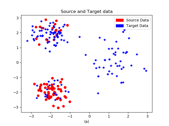
Let and be the conditional distributions of source and target respectively with possibly for . Similarly we denote the marginal source and target distributions as and . Our goal is to learn a distribution alignment scheme able to reject from the samples of the unknown class while matching correctly the remaining source and target samples by accounting for the label-shift and possibly a shift in the conditional distributions. For this, we propose a two-step approach (see in Fig. 2 in the appendix 0.A.6 for an illustration): a rejection step followed by the label shift correction. To proceed we rely on discrete OT framework which is introduced hereafter.
3.1 The general optimal transport framework
This section reviews the basic notions of discrete OT and fixes additional notation. Let be the probability simplex with bins, namely the set of probability vectors in i.e., . Let and be two discrete distributions derived respectively from and such that
where stands for the probability mass associated to the -th sample (the same for ). Computing OT distance between and , referred to as the Monge-Kantorovich or Wasserstein distance [14, 26]. amounts to solving the linear problem given by
| (1) |
where denotes Frobenius product between two matrices, that is . Here the matrix , where each represents the energy needed to move a probability mass from to . In our setting is given by the pairwise Euclidean distances between the instances in the source and target distributions, i.e., . The matrix is called a transportation plan, namely each entry represents the fraction of mass moving from to . The minimum ’s in problem (1) is taken over the convex set of probability couplings between and defined by
where we identify the distributions with their probability mass vectors, i.e. (similarly for , and stands for all-ones vector. The set contains all possible joint probabilities with marginals corresponding to and In the sequel when applied to matrices and vectors, product, division and exponential notations refer to element-wise operators.
Computing classical Wassertein distance is computationally expensive, since its Kantorovich fomulation (1) is a standard linear program with a complexity [15]. To overcome this issue, a prevalent approach, referred to as regularized OT [9], operates by adding an entropic regularization penalty to the original problem and it writes as
| (2) |
where defines the entropy of the matrix and is a regularization parameter to be chosen. Adding the entropic term makes the problem significantly more amenable to computations. In particular, it allows to solve efficiently the optimization problem (2) using a balancing algorithm known as Sinkhorn’s algorithm [25]. Note that the Sinkhorn iterations are based on the dual solution of (2) (see [18] for more details).
3.2 First step: Rejection of unknown class samples
In the open set DA setting, a naive application of the preceding OT framework to source set and target dataset will lead to undesirable mappings as some source samples will be transported onto the abnormal target samples. To avoid this, we intend to learn a transportation map such that the probability mass sent to the unknown abnormal samples of the target domain will be negligible, hence discarding those samples. A way to achieve this goal is to adapt the target marginal distribution while learning the map.
Therefore, to discard the new classes appearing in the target domain, in a first stage, we solve the following optimization problem:
| (3) |
where stands for the target marginal and for the source one .
The first stage of the rejection step as formulated in (3) aims at calculating a transportation plan while optimizing the target marginal . The rationale for updating is linked to the new classes appearing in target domain. Therefore, the formulation allows some freedom on and leads to more accurate matching between known marginal source and unknown marginal target. To solve this optimization problem, we use Sinkhorn iterations [9]. Towards this end, we explicit its dual form in Lemma 1. Hereafter, we set where stands for the Gibbs kernel associated to the cost matrix and where diag denotes the diagonal operator.
Lemma 1
Note that the optimal solutions and of the primal problem take the form
Once is learned, the second stage consists in discarding the new classes by relying on the values of . Specifically, we reject the -th sample in the target set whenever is a neglectable value with respect to some chosen threshold. Indeed, since satisfies the target marginal constraint for all , we expect that the row entries take small values for each -th sample associated to a new class, that is we avoid transferring probability mass from source samples to the unknown target -th instance. The tuning of the rejection threshold is exposed in Section 4.1.
The overall rejection procedure is depicted in Algorithm 1. To grasp the elements of Algorithm 1 and its stopping condition, we derive the Karush-Kuhn-Tucker (KKT) optimality conditions [5] for the rejection dual problem (Eq. 4) in Lemma 2.
Lemma 2
We remark that we have a closed form of , see Eq. 5, while it is not the case for as shown in Eq. 6. This is due to non-differentiability of the objective function defining the couple . Therefore, we tailor Algorithm 1 with a sufficient optimality condition to guarantee Eq. 6, in particular we set for all . These latter conditions can be tested on the update of the target marginal for the rejection problem (see Steps 6-9 in Algorithm 1). We use the condition (-tolerance) as a stopping criterion for Algorithm 1, which is very natural since it requires that and are close to the source and target marginals and
require: : regularization parameter, : cost matrix, : target samples, : number of source samples, : number of target samples,
tol: tolerance, thresh: threshold;
output: transport matrix: ; target marginal: rejected samples:
3.3 Second step: Label-Shift correction
We re-weight source samples to correct the difference in class proportions between source and target domains. Correcting the label shift is formulated as
| (7) |
where the target marginal is either a uniform distribution or the one learned at the rejection step and where is a linear operator, such that for and
Here denotes the cardinality of source samples with class , namely The parameter vector belongs to the convex set
In order to estimate the unknown class proportions in the target domain, we set-up the source marginal as where the entry expresses the -class proportion for all Once we estimate theses proportions, we can get the class proportions in target domain thanks to OT matching. We shall stress that Problem (7) involves the simultaneous calculation of the transportation plan and the source class re-weighting. Our procedure resembles the re-weighting method of JCPOT [19] except that we do not rely on a Wasserstein barycentric problem required by the multiple source setting addressed in [19]. The estimation can be explicitly calculated using the source marginal constraint satisfied by the transportation plan , i.e.,
As for the rejection step, we use Sinkhorn algorithm with an update on the source marginal to solve the label shift Problem (7) via its dual as stated in Lemma 3.
Lemma 3
Moreover, the closed form of the transportation plan in the Label-Shift step is given by
The analysis details giving the dual formulation in Equation (8) in Lemma 3 are presented in the appendices. As for the rejection problem, the optimality conditions of the Label-Shift problem are described in the dedicated Lemma 4 which proof is differed to Appendix 0.A.3.
Lemma 4
Algorithm 2 shows the related optimization procedure. Similarly to the rejection problem, we see that admits a close form (Eq. 9), while does not. As previously, we endow the Algorithm 2 with the sufficient optimality conditions (10) by ensuring for all . The conditions are evaluated on the source marginal (see Steps 5-9 in Algorithm 2). Finally we use the same -tolerance stopping condition .
require: : regularization term; : cost matrix, : source labels, : number of source samples; : number of target samples; : number of classes;
tol: tolerance;
D: linear operator;
output: transport matrix: ; class proportions: ; Prediction of target labels:
3.4 Implementation details and integration
Our proposed approach to open set DA performs samples rejection followed by sample matching in order to predict the target labels (either outlier or known source domain label). Hence, at the end of each step, we identify either rejected samples or predict target labels (see Step 14 of Algorithms 1 and 2).
For rejection, we compare the learned target marginal to some threshold to recognize the rejected samples (See Section 4.1 for its tuning). To fix the threshold, we assume that the target samples that receive insufficient amount of probability mass coming from source classes likely cannot be matched to any source sample and hence are deemed outliers.
To predict the labels of the remaining target samples, we rely on the transportation map given by Algorithm 2. Indeed for Label-Shift, JCPOT [19] suggested a label propagation approach to estimate labels from transportation maps (corresponding to source domains). Following JCPOT, the obtained transport matrix is proportional to the target class proportions. Therefore, we estimate the labels of the target samples based on the probability mass they received from each source class using . The term provides a matrix of mass distribution over classes.
Finally, we stress that the rejection and Label-Shift steps are separately done allowing us to compare theses approaches with the sate-of-art. Nevertheless, we can make a joint 2-step, that means after rejecting the instances with new classes in the target domain we plug the obtained target marginal in the Label-Shift step. Experimental evaluations show that similar performances are attained for separate and joint steps.
4 Numerical experiments
To assess the performance of each step, we first present the evaluations of Rejection and Label-Shift algorithms so that we can compare them to state-of-the-art approaches. Then we present overall accuracy of the joint 2-step algorithm.
4.1 Abnormal sample rejection
We frame the problem as a binary classification where common and rejected classes refer respectively to positive and negative classes. Therefore, source domain has only one class (the positive) while target domain includes a mixture of positives and negatives. We estimate their proportions and compare our results to open set recognition algorithms for unknown classes detection.
To reject the target samples, we lay on the assumption that they correspond to entries with a small value in . The applied threshold to these entries is strongly linked to the regularization parameter of the OT problem (3). We remark that when increases, the threshold is high and vice versa, making the threshold proportional to . Also experimentally, we notice that the threshold has the same order of magnitude of . Therefore, we define a new hyper-parameter such that the desired treshold is given by .
In order to fix the hyper-parameters (,) of the Rejection algorithm, we resort to Reverse Validation procedure [6, 30]. For a standard classification problem where labels are assumed to be only available for source samples, a classifier is trained on in the forward pass and evaluated on to predict . In the backward pass, the target samples with the pseudo-labels are used to retrain the classifier with the same hyper-parameters used during the first training, to predict . The retained hyper-parameters are the ones that provide the best accuracy computed from without requiring .
We adapt the reverse validation principle to our case. For fixed , Algorithm 1 is run to get and to identify abnormal target samples. These samples are removed from leading to . Then the roles of and are reversed. By running the Rejection algorithm to map onto we expect that the yielded marginal will have entries greater than the threshold . This suggests that we did not reject erroneously the target samples during the forward pass. As we may encounter mis-rejection, we select the convenient hyper-parameters (,) that correspond to the highest . Algorithm 3 in Appendix 0.A.5 gives the implementation details of the adapted Reverse Validation approach.
We use a grid search to find optimal hyperparameters (,). was searched in the following set {0.001,0.01,0.05,0.1,0.5,1,5,10} and in {0.1,1,10}. We apply Algorithm 3 and get and for synthetic data and and for real datasets.
Experiments on synthetic datasets
We use a mixture of 2D Gaussian dataset with classes. We choose or classes to be rejected in target domain as shown in Table 1. We generate samples for each class in both domains with varying noise levels.
The change of rejected classes at each run induces a distribution shift between shared (Sh) and rejected (Rj) class proportions. Tables 1 and 2 present the recorded F1-score. For a fair comparison, we tune the hyper-parameters of the competitor algorithms and choose the best F1-score for each experiment.
| Sh classes | {0,1} | {0,2} | {1,2} | {0} | {1} | {2} |
|---|---|---|---|---|---|---|
| Rj classes | {2} | {1} | {0} | {1,2} | {0,2} | {0,1} |
| % of Rj classes | 33% | 33% | 33% | 66% | 66% | 66% |
| 1Vs (Linear) | 0.46 | 0.5 | 0 | 0 | 0 | 0 |
| WSVM (RBF) | 0.99 | 0.99 | 0.99 | - | - | - |
| PISVM (RBF) | 0.99 | 0.99 | 0.69 | 0.5 | 0.5 | 0.5 |
| Ours | 1 | 0.99 | 0.99 | 1 | 1 | 0.98 |
| Sh classes | {0,1} | {0,2} | {1,2} | {0} | {1} | {2} |
|---|---|---|---|---|---|---|
| Rj classes | {2} | {1} | {0} | {1,2} | {0,2} | {0,1} |
| % of Rj classes | 33% | 33% | 33% | 66% | 66% | 66% |
| 1Vs (Linear) | 0.5 | 0.37 | 0.49 | 0 | 0 | 0 |
| WSVM (RBF) | 0.81 | 0.8 | 0.79 | - | - | - |
| PISVM (RBF) | 0.94 | 0.83 | 0.8 | 0.5 | 0.5 | 0.5 |
| Ours | 0.95 | 0.96 | 0.97 | 0.98 | 0.98 | 0.96 |
Experiments on real datasets
For this step, we first evaluate our rejection algorithm on datasets under Label-Shift and open set classes. We modify the set of classes for each experiment in order to test different proportions of rejected class. We use USPS (U), MNIST (M) and SVHN (S) benchmarks. All the benchmarks contain 10 classes. USPS images have single channel and a size of pixels, MNIST images have single channel and a size of pixels while SVHN images have 3-color channels and a size of pixels.
As a first experiment, we sample our source and target datasets from the same benchmark i.e. USPS USPS, MNIST MNIST and SVHN MNIST. We choose different samples for each domain and modify the set of shared and rejected classes. Then, we present challenging cases with increasing Covariate- Shift as source and target samples are from different benchmarks as shown in Table 3. For each benchmark, we resize the images to pixels and split source samples into training and test sets. We extract feature embeddings using the following process : 1) We train a Neural Network (as suggested in [12]) on the training set of source domain, 2) We randomly sample 200 images (except for USPS 72 images instead) for each class from test set of source and target domains, and 3) We extract image embeddings of chosen samples from the last Fc layer (128 units) of the trained model.
We compare our Rejection algorithm to the -Vs Machine [24] , PISVM [13] and WSVM [23]11 1 https://github.com/ljain2/libsvm-openset which are based on SVM and require a threshold to provide a decision. For tasks with a single rejected class, we get results similar to PISVM and WSVM when noise is small (Table 1) and outperfom all methods when noise increases (Table 2). These results prove that we are more robust to ambiguous dataset. For tasks with multiple rejected classes, WSVM is not suitable to this case and PISVM and 1Vs performs poorly compared to our approach. In fact, these approaches strongly depend on openness measure [13, 23].
As for the case with small noise, we obtain similar results for DA tasks with Label-Shift only as shown in Table 3 while we outperform state-of-art methods for DA tasks combining target and covariate shifts (Table 4) except for last task where WSVM slightly exceeds our method. This confirms the ability of our approach to address challenging shifts. In addition, our proposed approach for the rejection step is based on OT which provides a framework consistent with the Label-Shift step.
| Sh classes | {0,2,4} | {6,8} | {1,3,5} | {7,9} | {0,1,2,3,4} |
|---|---|---|---|---|---|
| Rj classes | {6,8} | {0,2,4} | {7,9} | {1,3,5} | {5,6,7,8,9} |
| % of Rj classes | 40% | 60% | 40% | 60% | 50% |
| 1Vs (Linear) | 0.65 0.01 | 0 | 0.74 0.01 | 0.29 0.04 | 0.61 |
| WSVM (RBF) | 0.97 0.02 | 0.95 0.0 | 0.98 0.01 | 0.76 0.2 | 0.96 0.01 |
| PISVM (RBF) | 0.98 0.01 | 0.96 0.02 | 0.98 0.01 | 0.80 0.16 | 0.97 0.01 |
| Ours | 0.98 0.01 | 0.99 0.01 | 0.98 0.01 | 0.97 0.01 | 0.93 0.02 |
| Sh classes | {0,2,4} | {6,8} | {1,3,5} | {7,9} | {0,1,2,3,4} |
|---|---|---|---|---|---|
| Rj classes | {6,8} | {0,2,4} | {7,9} | {1,3,5} | {5,6,7,8,9} |
| % of Rj classes | 40% | 60% | 40% | 60% | 50% |
| 1Vs (Linear) | 0.57 0.04 | 0 | 0.62 0.05 | 0.27 0.06 | 0.53 0.04 |
| WSVM (RBF) | 0.82 0.09 | 0.69 0.07 | 0.86 0.05 | 0.64 0.06 | 0.79 0.04 |
| PISVM (RBF) | 0.82 0.09 | 0.68 0.06 | 0.86 0.05 | 0.66 0.06 | 0.77 0.04 |
| Ours | 0.9 0.02 | 0.83 0.03 | 0.87 0.05 | 0.92 0.02 | 0.74 0.06 |
4.2 Label-Shift
We sample unbalanced source datasets and reversely unbalanced target datasets for both MNIST and SVHN benchmarks in order to create significant Label-Shift as shown in Fig. 1 in Appendix 0.A.4. USPS benchmark is too small (2007 samples for test) and is already unbalanced. Therefore we use all USPS samples for the experiments MU and UM.
We create 5 tasks by increasing Covariate-Shift to evaluate the robustness of our algorithm. We compare our approach to JDOT [7] and JCPOT [19] which predicts target label in two different ways (label propagation JCPOT-LP and JCPOT-PT). We used the public code given by the authors for JDOT22 2 Code available at https://github.com/rflamary/JDOT and JCPOT33 3 Code available at https://github.com/ievred/JCPOT. Note that JCPOT is applied to multi-source samples. Consequently,we split {} into sources with random class proportions and chose which gives the best results (N=5). We present the results on 5 trials. We set for all experiments with the Label-Shift algorithm. JCPOT uses a grid search to get its optimal .
For synthetic dataset, JCPOT and our Label-Shift method give similar results (Table 5). However, for real datasets as shown in Table 6, we widely outperform other state-of-the-art DA methods especially for DA tasks that present covariate shift in addition to the Label-Shift. These results prove that our approach is more robust to high-dimensional dataset as well as to distributions with combined label and covariate shifts.
| Setting | JDOT | JCPOT-LP(5) | JCPOT-PT(5) | Ours |
|---|---|---|---|---|
| Noise = 0.5 | 0.5 | 0.997 | 0.99 | 0.997 |
| Noise = 0.75 | 0.45 | 0.98 | 0.94 | 0.98 |
| Methods | MM | SS | MU | UM | SM |
|---|---|---|---|---|---|
| JDOT | 0.52 0.04 | 0.53 0.01 | 0.64 0.01 | 0.87 0.02 | 0.43 0.01 |
| JCPOT-LP(5) | 0.98 0.002 | 0.37 0.43 | 0.56 0.0.026 | 0.89 0.01 | 0.21 0.237 |
| JCPOT-PT(5) | 0.96 0.004 | 0.81 0.045 | 0.40 0.327 | 0.86 0.013 | 0.46 0.222 |
| Ours | 0.98 0.001 | 0.92 0.006 | 0.76 0.019 | 0.92 0.006 | 0.65 0.017 |
4.3 Full 2-step approach: Rejection and Label-Shift
The same shared and rejected classes from the rejection experiments tasks have been chosen. We also create significant Label-Shift as done for Label-Shift experiments (Unbalanced and Reversely-unbalanced class proportions) for synthetic datasets as well as for MNIST and SVHN real benchmarks. Nevertheless, we keep the initial class proportions of USPS due to the size constraint of the database. This time, we implement a jointly 2-step. Namely, we plug the obtained target marginal in the Label-Shift step after discarding rejected samples. We apply Algorithm 3 to rejection step to get optimal hyperparameters (,) and keep the same for Label-shift step. We obtained and .
In Table 7, we show results for synthetic data generated with different noises. When noise increases, i.e., boundary decision between classes is ambiguous, the performance is affected. Table 8 presents F1-score over 10 runs of our 2-step approach applied to real datasets. For DA tasks with only Label-Shift (MM and SS), F1-score is high. However it drops when we address both Covariate and Label-Shift (MU, UM and SM). In fact, previous results for each step (Tables 4 and 6) have shown that performance was affected by Covariate-Shift. The final result of our 2-step approach is linked to the performance of each separate step. We present an illustration of the full algorithm in Fig. 2 in Appendix 0.A.6.
| Sh classes | {0,1} | {0,2} | {1,2} |
|---|---|---|---|
| Rj classes | {2} | {1} | {0} |
| Noise = 0.5 | 1 | 0.99 | 0.99 |
| Noise = 0.75 | 0.93 | 0.87 | 0.85 |
| Benchmarks | MM | SS | MU | UM | SM |
|---|---|---|---|---|---|
| Sh {0,2,4} | 0.93 0.005 | 0.91 0.008 | 0.65 0.011 | 0.59 0.014 | 0.66 0.011 |
| Rj {6,8} | |||||
| Sh {6,8} | 0.95 0.006 | 0.89 0.012 | 0.82 0.013 | 0.61 0.01 | 0.53 0.014 |
| Rj {0,2,4} | |||||
| Sh {1,3,5} | 0.93 0.009 | 0.86 0.01 | 0.76 0.02 | 0.58 0.011 | 0.74 0.018 |
| Rj {7,9} | |||||
| Sh {7,9} | 0.97 0.009 | 0.90 0.011 | 0.75 0.008 | 0.52 0.007 | 0.65 0.021 |
| Rj {1,3,5} | |||||
| Sh {0,1,2,3,4} | 0.91 0.01 | 0.82 0.007 | 0.73 0.013 | 0.74 0.01 | 0.68 0.01 |
| Rj {5,6,7,8,9} |
5 Conclusion
In this paper, we proposed an optimal transport framework to solve open set DA. It is composed of two steps solving Rejection and Label-shift adaptation problems. The main idea was to learn the transportation plans together with the marginal distributions. Notably, experimental evaluations showed that applying our algorithms to various datasets lead to consistent outperforming results over the state-of-the-art. We plan to extend the framework to learn deep networks for open set domain adaptation.
Acknowledgements
This work was supported by the National Research Fund, Luxembourg (FNR) and the OATMIL ANR-17-CE23-0012 Project of the French National Research Agency (ANR).
References
- [1] Arjovsky, M., Chintala, S., Bottou, L.: Wasserstein generative adversarial networks. In: Proceedings of the 34th International Conference on Machine Learning. vol. 70, pp. 214–223 (2017)
- [2] Ben-David, S., Blitzer, J., Crammer, K., Kulesza, A., Pereira, F., Vaughan, J.: A theory of learning from different domains. Machine Learning 79, 151–175 (2010)
- [3] Bhushan Damodaran, B., Kellenberger, B., Flamary, R., Tuia, D., Courty, N.: Deepjdot: Deep joint distribution optimal transport for unsupervised domain adaptation. In: Proceedings of the ECCV. pp. 447–463 (2018)
- [4] Bonneel, N., Van De Panne, M., Paris, S., Heidrich, W.: Displacement interpolation using lagrangian mass transport. In: Proceedings of the 2011 SIGGRAPH Asia Conference. pp. 1–12 (2011)
- [5] Boyd, S., Vandenberghe, L.: Convex Optimization. Cambridge University Press (2004)
- [6] Bruzzone, L., Marconcini, M.: Domain adaptation problems: A dasvm classification technique and a circular validation strategy. IEEE Transactions on Pattern Analysis and Machine Intelligence 32(5), 770–787 (2010)
- [7] Courty, N., Flamary, R., Habrard, A., Rakotomamonjy, A.: Joint distribution optimal transportation for domain adaptation. In: Advances in Neural Information Processing Systems. pp. 3730–3739 (2017)
- [8] Courty, N., Flamary, R., Tuia, D., Rakotomamonjy, A.: Optimal transport for domain adaptation. IEEE transactions on pattern analysis and machine intelligence 39(9), 1853–1865 (2016)
- [9] Cuturi, M.: Sinkhorn distances: Lightspeed computation of optimal transport. In: Burges, C.J.C., Bottou, L., Welling, M., Ghahramani, Z., Weinberger, K.Q. (eds.) Advances in Neural Information Processing Systems 26. pp. 2292–2300 (2013)
- [10] Fang, Z., Lu, J., Liu, F., Xuan, J., Zhang, G.: Open set domain adaptation: Theoretical bound and algorithm. arXiv preprint arXiv:1907.08375 (2019)
- [11] Ganin, Y., Ustinova, E., Ajakan, H., Germain, P., Larochelle, H., Laviolette, F., Marchand, M., Lempitsky, V.: Domain-adversarial training of neural networks. The Journal of Machine Learning Research 17(1), 2096–2030 (2016)
- [12] Haeusser, P., Frerix, T., Mordvintsev, A., Cremers, D.: Associative domain adaptation. In: The IEEE ICCV (Oct 2017)
- [13] Jain, L.P., Scheirer, W.J., Boult, T.E.: Multi-class open set recognition using probability of inclusion. In: Fleet, D., Pajdla, T., Schiele, B., Tuytelaars, T. (eds.) Computer Vision – ECCV 2014. pp. 393–409 (2014)
- [14] Kantorovich, L.: On the transfer of masses (in russian). Doklady Akademii Nauk 2, 227–229 (1942)
- [15] Lee, Y.T., Sidford, A.: Path finding methods for linear programming: Solving linear programs in o (vrank) iterations and faster algorithms for maximum flow. In: 2014 IEEE 55th Annual Symposium on Foundations of Computer Science. pp. 424–433 (2014)
- [16] Lipton, Z.C., Wang, Y., Smola, A.J.: Detecting and correcting for label shift with black box predictors. In: Proceedings of the 35th International Conference on Machine Learning (2018)
- [17] Panareda Busto, P., Gall, J.: Open set domain adaptation. In: Proceedings of the IEEE International Conference on Computer Vision. pp. 754–763 (2017)
- [18] Peyré, G., Cuturi, M.: Computational optimal transport. Foundations and Trends® in Machine Learning 11(5-6), 355–607 (2019)
- [19] Redko, I., Courty, N., Flamary, R., Tuia, D.: Optimal transport for multi-source domain adaptation under target shift. In: Proceedings of Machine Learning Research. vol. 89, pp. 849–858 (2019)
- [20] Redko, I., Habrard, A., Sebban, M.: Theoretical analysis of domain adaptation with optimal transport. In: Joint European Conference on Machine Learning and Knowledge Discovery in Databases. pp. 737–753 (2017)
- [21] Saito, K., Yamamoto, S., Ushiku, Y., Harada, T.: Open set domain adaptation by backpropagation. In: Proceedings of the ECCV. pp. 153–168 (2018)
- [22] Sanderson, T., Scott, C.: Class proportion estimation with application to multiclass anomaly rejection. In: Artificial Intelligence and Statistics. pp. 850–858 (2014)
- [23] Scheirer, W.J., Jain, L.P., Boult, T.E.: Probability models for open set recognition. IEEE Transactions on Pattern Analysis and Machine Intelligence 36(11), 2317–2324 (2014)
- [24] Scheirer, W., Rocha, A., Sapkota, A., Boult, T.: Toward open set recognition. IEEE transactions on pattern analysis and machine intelligence 35, 1757–72 (07 2013)
- [25] Sinkhorn, R.: Diagonal equivalence to matrices with prescribed row and column sums. The American Mathematical Monthly 74(4), 402–405 (1967)
- [26] Villani, C.: Topics in Optimal Transportation. Graduate studies in mathematics, American Mathematical Society (2003)
- [27] Wu, Y., Winston, E., Kaushik, D., Lipton, Z.: Domain adaptation with asymmetrically-relaxed distribution alignment. In: International Conference on Machine Learning. pp. 6872–6881 (2019)
- [28] Zhang, K., Schölkopf, B., Muandet, K., Wang, Z.: Domain adaptation under target and conditional shift. In: International Conference on Machine Learning. pp. 819–827 (2013)
- [29] Zhao, H., Combes, R.T.D., Zhang, K., Gordon, G.: On learning invariant representations for domain adaptation. In: Proceedings of the 36th International Conference on Machine Learning. vol. 97, pp. 7523–7532 (2019)
- [30] Zhong, E., Fan, W., Yang, Q., Verscheure, O., Ren, J.: Cross validation framework to choose amongst models and datasets for transfer learning. In: Balcázar, J.L., Bonchi, F., Gionis, A., Sebag, M. (eds.) Machine Learning and Knowledge Discovery in Databases. pp. 547–562 (2010)
Appendix 0.A Appendix
0.A.1 Proof of Lemma 1
Define the dual Lagrangian function
equivalently
where
We have
and
Then the couple optimum of the dual Lagrangian function satisfies the following
for all and Now, plugging this solution in the Lagrangian function we get
Note that , hence taking into account the constraint for all it entails that Hence
subject to for all Setting the following variable change and we get
Then
subject to . Putting , then . This gives
subject to , for all We remark that
then using a variable change and we get
Therefore
0.A.2 Proof of Lemma 2
Setting
Writting the KKT optimlaity condition for the above problem leads to the following: we have is differentiable, hence we can calculate a gradient with respect to . However is not differentiable, then we just calculate a subdifferentiale as follows:
and
where is the subdifferential of the indicator function at is known as the normal cone, namely
Therefore, KKT optimality conditions give
(the division and the multiplcation between vectors have to be understood elementwise). So
equivalently
for all
0.A.3 Proof of Lemma 3
First, observe that Then the dual Lagrangian function is given by
equivalently
where
We have
and
Then the couple optimum of the dual Lagrangian function satisfies the following
for all , and Now, plugging this solution in the Lagrangian function we get
Observe that
Taking into account the constraint for all it entails that Hence
subject to for all Setting the following variable change and we get
Then
subject to , for all Putting , then . This gives
subject to , for all We remark that
then using a variable change and we get
Finally
that is
0.A.4 Unbalancement trade-off

0.A.5 Reverse validation details
require: : list of suggested regularization terms; : list of values to fix threshold, : source samples; : target samples; : number of source samples; : number of target samples;
output: : tuple of hyperparameters;
0.A.6 Algorithm Illustration