Displaced Vertex signatures of a pseudo-Goldstone
sterile neutrino
Stéphane Lavignaca,11 1 stephane.lavignac@ipht.fr and Anibal D. Medinab,22 2 anibal.medina@fisica.unlp.edu.ar
aInstitut de Physique Théorique, Université Paris Saclay, CNRS, CEA,
F-91191 Gif-sur-Yvette, France
bIFLP, CONICET - Dpto. de Física, Universidad Nacional de La Plata,
C.C. 67, 1900 La Plata, Argentina
Abstract
Low-scale models of neutrino mass generation often feature sterile neutrinos with masses in the GeV-TeV range, which can be produced at colliders through their mixing with the Standard Model neutrinos. We consider an alternative scenario in which the sterile neutrino is produced in the decay of a heavier particle, such that its production cross section does not depend on the active-sterile neutrino mixing angles. The mixing angles can be accessed through the decays of the sterile neutrino, provided that they lead to observable displaced vertices. We present an explicit realization of this scenario in which the sterile neutrino is the supersymmetric partner of a pseudo-Nambu-Goldstone boson, and is produced in the decays of higgsino-like neutralinos and charginos. The model predicts the active-sterile neutrino mixing angles in terms of a small number of parameters. We show that a sterile neutrino with a mass between a few and can lead to observable displaced vertices at the LHC, and outline a strategy for reconstructing experimentally its mixing angles.
1 Introduction
The existence of heavy sterile neutrinos is predicted by many models of neutrino mass generation, such as the seesaw mechanism[1, 3, 2] and its various incarnations. In the standard, GUT-inspired picture, these heavy neutrinos have a mass and order one Yukawa couplings , thus providing a natural explanation for the smallness of the Standard Model neutrino masses through the seesaw formula . However, there is no model-independent prediction for the masses of the sterile neutrinos – they could range from the GUT scale to the eV scale, or even below. Of particular interest are sterile neutrinos with a mass between the GeV and the TeV scales, which can lead to observable signatures at colliders (for reviews, see e.g. Refs. [4, 5]). Most phenomenological studies and experimental searches assume a single sterile neutrino , which is produced through its mixing with the active (Standard Model) neutrinos, parametrized by mixing angles , where is the active lepton flavour. Since the enter the sterile neutrino production cross section, they can be measured directly, unless they are too small to give a detectable signal.
In this work, we consider an alternative production mechanism for the sterile neutrino that does not depend on the active-sterile neutrino mixing angles. Instead, the sterile neutrino is produced in the decay of a heavier particle, whose production cross section is of typical electroweak size. The mixing angles can be determined from the subsequent decays of the sterile neutrino, provided that its total decay width is measured independently. This can be done if the sterile neutrino decays are not prompt (as expected if the active-sterile neutrino mixing is small), in which case the decay width can be extracted from the distribution of displaced vertices. We show that it is possible to probe values of the that would be out of reach if the production cross section were suppressed by the active-sterile neutrino mixing, as usually assumed. We study an explicit realization of this scenario in which the sterile neutrino is the supersymmetric partner of the pseudo-Nambu Goldstone boson of a spontaneously broken global symmetry. This “pseudo-Goldstone” sterile neutrino is produced in the decays of higgsino-like neutralinos and charginos and decays subsequently via its mixing with the active neutrinos. We outline an experimental strategy for measuring the active-sterile neutrino mixing angles at the LHC, based on the reconstruction of final states involving displaced vertices.
The paper is organized as follows. In Section 2, after a brief summary of current collider constraints, we introduce the sterile neutrino production mechanism studied in this work and contrast it with the standard one. In Section 3, we present an explicit model in which the sterile neutrino is the supersymmetric partner of a pseudo-Nambu Goldstone boson, and give its predictions for the active-sterile neutrino mixing angles. In Section 4, we study the experimental signatures of the model and discuss how the active-sterile neutrino mixing angles could be reconstructed experimentally. We give our conclusions in Section 5. Finally, Appendix A contains some technical details about the model of Section 3, and Appendix B discusses the phenomenological constraints that apply to the pseudo-Nambu-Goldstone boson whose supersymmetric partner is the sterile neutrino.
2 Sterile neutrino production in heavy particle decays
Collider searches for heavy sterile neutrinos usually rely on a production mechanism involving their mixing with the active neutrinos11 1 Except for searches performed in the framework of specific scenarios, like left-right symmetric extensions of the Standard Model, in which the right-handed neutrinos are produced in decays of or gauge bosons [6]. In this case, the production cross section is controlled by the gauge coupling and does not depend on the active-sterile neutrino mixing.. The active-sterile mixing angles can be measured directly, as they enter the production cross section. Following this approach, early direct searches for heavy sterile neutrinos were performed by the DELPHI experiment [7] at the LEP collider. These searches were based on the production process , followed by the decay or . Since the coupling is proportional to the active-sterile mixing angle (where or ), the production cross section goes as . This allowed DELPHI to exclude mixing angles for sterile neutrino masses in the range , independently of lepton flavour [7]. DELPHI was also able to set limits on the for lower sterile neutrino masses, using techniques involving displaced vertices. For , a stronger, indirect constraint can be derived from the non-observation of neutrinoless double beta decay [8, 9].
At hadron colliders, the production process , followed by the decay , leads to the same-sign dilepton + 2 jets signature with no missing transverse energy characteristic of a heavy Majorana neutrino [6, 10], which is essentially free from Standard Model backgrounds. The boson from decay can also go into a charged lepton and a neutrino, resulting in a trilepton signature. Similarly to , the coupling is proportional to and the production cross section goes as . More precisely, the cross section for the process mediated by -channel boson exchange is given by, at a center of mass energy [11],
| (1) |
where , , is the parton distribution function for the quark at , and and are the fractions of the proton momentum carried by the interacting quark and antiquark . The parton subprocess cross section is given by
| (2) |
where , with the gauge coupling. The collaborations ATLAS and CMS performed searches for heavy sterile neutrinos at , using events with two jets and two leptons of the same charge, and set -dependent upper bounds on and in the mass range for ATLAS [12], and for CMS [13, 14]. The best limits were obtained by CMS, ranging from , for to , for , with , around . Using trilepton events with 35.9 fb-1 of proton-proton collisions at TeV, CMS extended these constraints to the mass range , providing upper bounds on and ranging from to the unphysical value , depending on [15]. In particular, CMS slightly improved the DELPHI limits between and . Using the same trilepton signature with 36.1 fb-1 of proton-proton collisions at TeV, ATLAS obtained bounds similar to CMS in the mass range , excluding between and . By searching for displaced vertex signatures with a displacement between and , ATLAS was also able to probe values of below in the mass range , excluding for .
The possibility of probing smaller mixing angles via displaced vertex searches at the LHC (allowing for larger displacements than in the ATLAS study just mentioned) has been investigated in several phenomenological works [17, 18, 19, 20, 21, 22, 23, 24, 25, 26, 27, 28, 29] (see also Ref. [30] for a more general discussion about signatures of long-lived particles at the LHC). The requirement that the sterile neutrino does not decay promptly, while being sufficiently produced through its mixing with the active neutrinos, restricts the sensitivity of these searches to the low mass region, , depending on the available luminosity22 2 Roughly speaking, the sterile neutrino production cross section is proportional to , while its decay rate goes as . The requirement that a significant number of sterile neutrinos are produced implies a lower bound on , while the requirement of displaced vertices provides and upper bound on the combination .. For instance, Ref. [26] claims that displaced vertex searches at the LHC could exclude values of and as small as and masses up to with an integrated luminosity of , while the high luminosity LHC (HL-LHC) with an integrated luminosity of could probe and . The sensitivity to is typically smaller by two orders of magnitude.
It is interesting to compare the above limits and sensitivities to the predictions of typical GeV/TeV-scale seesaw models. Using the naïve seesaw formula , one obtains for , and for , about seven orders of magnitude below the best collider bounds. Even displaced vertex searches at the LHC or HL-LHC do not seem to have the potential to reach the vanilla seesaw model predictions and, moreover, are limited to sterile neutrino masses below . All these searches are handicapped by the fact that the sterile neutrino production cross section is suppressed by the square of the active-sterile mixing. This prevents them from probing smaller mixing angles and, in the case of displaced vertex searches, larger sterile neutrino masses.
In this paper, we consider the alternative possibility that the sterile neutrino production mechanism does not depend on its mixing with active neutrinos. In this case, the sensitivity of collider searches to small mixing angles is not limited by the production rate, as the mixing only enters the sterile neutrino decays. More specifically, we assume that the sterile neutrino is produced in the decays of a heavier particle , whose production cross sections is of typical electroweak size33 3 Another possibility, namely the production of a pair of sterile neutrinos in the decay of a gauge boson, was considered in Refs. [31, 32, 33].. This requires that the sterile neutrino mixes with , in addition to its mixing with active neutrinos. We further assume that is produced in pairs, a property encountered in many extensions of the Standard Model, where a parity symmetry is often associated with the new particles. Sterile neutrinos are then produced as follows:
| (3) |
where “SM” stands for Standard Model particles. If , these particles are boosted and can be used as triggers for the signal of interest. Consider for instance the production of two sterile neutrinos followed by their decay into a charged lepton and two jets, . The rate for this process is given by
| (4) |
where, assuming that the narrow width approximation is valid (i.e. ),
| (5) |
Eqs. (4) and (5) clearly show that the active-sterile mixing angles enter only the sterile neutrino decays, not its production. This makes small mixing angles more easily accessible to collider searches than in the standard scenario, in which the sterile neutrino is produced through its mixing with active neutrinos. As can be seen from Eq. (4), the number of events corresponding to a given final state depends on the combinations . An independent determination of is therefore needed in order to extract the from experimental data. This can be done by measuring the distribution of displaced vertices from decays, as we explain below. Another virtue of displaced vertices is that they provide signals which are essentially background free. Indeed, Standard Model processes do not lead to displaced vertices (with the exception of bottom and charm quarks, which produce small displacements and can be tagged). This implies that a small number of events may be sufficient to measure the signal.
To conclude this section, let us explain how the sterile neutrino decay width can be determined from the distribution of its displaced vertices. The probability density for a particle travelling in a straight line to decay at a distance to a particular final state is given by
| (6) |
where is the corresponding decay rate, the particle decay width, and we recall that , with the 3-momentum of the particle and its mass. For an ensemble of identical particles, one needs to integrate over the particle momentum distribution, on which depends. However, to a good approximation, one can simply assume that all particles have the same effective , given by the peak value of their distribution [34]. The number of particles decaying to the final state between and , with , is then given by
| (7) |
where is the initial number of particles. For two intervals , such that and , one can write
| (8) |
Thus, by measuring and the number of decays in two distance intervals, one can obtain the decay width of the particle in the approximation described above. More generally, i.e. without relying on the approximate formula (7), the decay width can be extracted from the shape of the distribution of displaced vertices corresponding to a given final state, provided that the mass and the momentum distribution of the particle (hence its distribution) can be reconstructed experimentally.
3 An explicit model: sterile neutrino as the supersymmetric partner of a pseudo-Nambu-Goldstone boson
We now present an explicit realization of the scenario discussed in the previous section. The sterile neutrino is identified with the supersymmetric partner of a pseudo-Nambu-Goldstone boson44 4 For earlier realizations of this idea, in which the sterile neutrino was assumed to be light, see Refs. [35, 36, 37, 38]. (PNGB) and mixes both with active neutrinos and higgsinos. Its mixing with higgsinos is relatively large, such that it is predominantly produced in neutralino and chargino decays.
3.1 The model
The model we consider is an extension of the Minimal Supersymmetric Standard Model (MSSM) with a global symmetry under which the lepton and Higgs fields (but not the quark fields) are charged. We assume that this symmetry is spontaneously broken at some high scale by the vacuum expectation value (VEV) of a scalar field belonging to a chiral superfield with charge (we also assume a small source of explicit breaking to avoid a massless Goldstone boson). The charges of the superfields , , and are denoted by , , and , respectively. We choose the symmetry to be generation-independent and vector-like, i.e. , in order to avoid dangerous flavor-changing processes [39] and astrophysical constraints on the pseudo-Nambu-Goldstone boson [40] (see Appendix B for details). We further assume , so that the top quark Yukawa coupling is invariant under the global symmetry and therefore unsuppressed by powers of the symmetry breaking parameter.
We are then left with two independent charges and , which we assume to be positive integers. With this choice, the down-type quark and charged lepton Yukawa couplings, as well as the -term, are not allowed by the global symmetry and must arise from higher-dimensional superpotential operators involving the field :
| (9) | |||||
where is the scale of the new physics that generates these operators. In the superpotential (9), we included terms that lead to -parity violating interactions, with the exception of the baryon number violating couplings , which we assume to be forbidden by some symmetry, such as the baryon parity of Ref. [41]. In principle, Eq. (9) should also contain a term , which after spontaneous symmetry breaking induces the Weinberg operator . We will discuss this contribution to neutrino masses later in this section.
The spontaneous breaking of the global symmetry generates the following superpotential55 5 In going from Eq. (9) to Eq. (10), we dropped the terms involving more than one power of , since, in addition to being suppressed by powers of the large scale , they do not contribute to the mixing between the pseudo-Goldstone fermion and the MSSM fermions. As we are going to see, it is this mixing that determines the collider phenomenology of the sterile neutrino.:
| (10) | |||||
where stands for the shifted superfiel and
| (11) |
in which . We will assume , such that the -parity violating parameters , , and are suppressed by a factor relative to the corresponding -parity conserving parameters:
| (12) |
where, for definiteness, we have assumed , and . -parity violation is therefore automatically suppressed by the choice of the charges; there is no need to invoke an ad hoc hierarchy between -parity even and -parity odd coefficients in the superpotential (9). Note that the coefficicents , and must have a hierarchical flavour structure in order to account for the fermion mass spectrum (this cannot be explained by the symmetry itself, since it is generation independent).
The chiral superfield contains the pseudo-Nambu-Goldstone boson and its supersymmetric partners. It can be written as:
| (13) |
where is the PNGB, its scalar partner, which is assumed to get a large mass from supersymmetry breaking, and its fermionic partner (hereafter referred to as the pseudo-Goldstone fermion or sterile neutrino), whose mass also predominantly arises from supersymmetry breaking. In particular, receives an irreducible contribution proportional to the gravitino mass [42]. By contrast, the pseudo-Nambu-Goldstone boson only obtains its mass from the sources of explicit global symmetry breaking, assumed to be small. The hierarchy of mass scales is therefore , and we will consider values of in the few 10 GeV to few 100 GeV range in the following. As discussed in Appendix B, is constrained to be larger than about by cosmological and astrophysical observations.
Before we can derive the interactions of the pseudo-Goldstone fermion, we must take into account the effect of supersymmetry breaking. Since -parity has not been imposed, the scalar potential includes soft supersymmetry breaking terms that violate -parity, which in turn induce vevs for the sneutrinos. After redefining the superfields and in such a way that (i) only the scalar component of gets a vev and (ii) charged lepton Yukawa couplings are diagonal, we end up with the following superpotential (see Appendix A for details):
| (14) |
where and are now the physical down-type Higgs and lepton doublet superfields. We have dropped the Yukawa couplings and the trilinear -parity violating couplings and , as they do not contribute to the mixing of the pseudo-Goldstone fermion with other fermions. As shown in Appendix A, the parameters , , and can be written as
| (15) |
where , is an overall measure of bilinear -parity violation defined in Appendix A, and , are order one coefficients (with ). We thus have the order-of-magnitude relations
| (16) |
Since and are small quantities, this implies and .
3.2 Sterile neutrino interactions
The superpotential (14) includes terms mixing the pseudo-Goldstone fermion with leptons, promoting it to a sterile neutrino. Since it is a gauge singlet, its interactions arise from its mixing with the other neutral fermions, namely the active neutrinos , the neutral higgsinos , and the gauginos , . This mixing is encoded in the () neutralino mass matrix, which in the 2-component fermion basis is given by
| (17) |
where , , and , are the VEVs of the two Higgs doublets of the supersymmetric Standard Model. The matrix contains small contributions to the mass terms arising from loops induced by the trilinear -parity violating couplings and , as well as from high-scale physics parametrized by the superpotential operators . The chargino mass matrix is given by, in the bases and ,
| (18) |
where are the charged lepton masses. The neutralino and chargino mass matrices are diagonalized by unitary matrices , and , which relate the mass eigenstates and to the gauge eigenstates and :
| (19) |
The neutralino mass matrix (17) has a “seesaw” structure, with the upper left block (associated with the MSSM neutralinos) containing the largest entries, while the elements of the off-diagonal block are suppressed by or , and the lower right block has as its largest entry, and being much smaller. Similarly, the chargino mass matrix (18) has a dominant upper left block corresponding to the MSSM charginos. This results in the following mass spectrum:
| (20) |
where and can be identified with the active neutrinos and charged leptons, respectively, is the sterile neutrino, and , are mostly the MSSM neutralinos and charginos. We therefore rename the mass eigenstates (20) in the following way:
| (21) |
Due to the specific hierarchical structure of the neutralino mass matrix, the sterile neutrino mass is approximately given by (). The hierarchy among the entries of and also implies that the mixing between states well separated in mass is small. As can be seen from Eq. (18), the mixing between charginos and charged leptons is suppressed by , while the mixing between the sterile neutrino, neutrinos and neutralinos has a more complicated structure and depends on the small parameters , and . These mixings induce new interactions between gauge bosons and fermions that are absent in the Standard Model. We will be interested in the ones that are relevant for the production and decay of the sterile neutrino, namely (assuming , such that the lightest neutralinos and chargino are mainly higgsinos):
| (22) |
All these couplings are suppressed by small mixing angles.
3.3 Constraints from neutrino data and active-sterile mixing angles
The model contains a large number of parameters (in addition to the supersymmetric parameters , , and , the chargino and neutralino mass matrices depend on , and (), or alternatively on , , and ). However, the requirement that it should be consistent with neutrino oscillation data fixes a lot of them. An efficient way of taking this constraint into account is to express the model parameters in terms of the neutrino parameters , and (where denotes the PMNS matrix, which controls flavour mixing in the lepton sector). In order to do this, we take advantage of the strongly hierarchical structure of the neutralino mass matrix (17) to derive the active neutrino mass matrix in the seesaw approximation:
| (23) |
where , , and the lepton family indices have been renamed from to to stress that we are working in the charged lepton mass eigenstate basis. For simplicity, we assume in the following, since its entries are small66 6 The superpotential terms give a contribution to the neutrino mass matrix. For the values of the model parameters considered in this paper: , and , this gives , which is too small to affect significantly the neutrino oscillation parameters. As for the lepton-slepton and quark-squark loops induced by the trilinear -parity violating couplings and , they are suppressed by and , respectively, which are smaller than , as shown in Appendix A. compared with the values suggested by neutrino oscillation data. With this choice, only two neutrinos become massive77 7 This can already be seen at the level of Eq. (17), whose determinant vanishes for .. We further assume that the neutrino mass ordering is normal, i.e. . Then the neutrino oscillation parameters are reproduced by the mass matrix (23) with
| (24) |
where and . This fixes the parameters and , as well as (as a function of , and ) and (as a function of , , and ). With the additional input of and the help of Eq. (15), the parameters and can be reconstructed. Thus, for a given set of neutrino parameters, the model has only five free parameters in the limit : , , , and . For the reference values , , and used in Section 4, one obtains and . Given the order-of-magnitude relation , this value of is consistent with the choice of “fundamental” parameters , and , which we adopt from now on. The value of corresponds to a global symmetry breaking scale .
Having traded some of the model parameters for the neutrino oscillation parameters, we can now derive a simple expression for the active-sterile neutrino mixing angles (still in the seesaw approximation):
| (25) |
For the current best fit values of the oscillation parameters [45, 46], this gives
| (26) |
In the approximation in which we are working, where all states heavier than the sterile neutrino are decoupled, these mixing angles enter the vertices and , i.e. the corresponding Lagrangian terms are . We checked numerically that this gives a very good approximation to the exact couplings, obtained by expressing the boson–fermion interactions in terms of the neutralino and chargino mass eigenstates. The approximation is less reliable for the individual couplings, but becomes very good after summing over the neutrino flavours.
In fact, Eq. (24) is not the most general solution to Eq. (23). Another solution is
| (27) |
giving
| (28) |
It is not difficult to show that the general solution is of the form
| (29) |
where is a complex orthogonal matrix88 8 Thus, in full generality, the model has seven free parameters in the limit : , , , , and a complex parameter parametrizing the matrix (strictly speaking, the parametrization of also involves a sign distinguishing between and ).. We will refer to Eq. (24) and Eq. (27) as the “maximal mixing” and “minimal mixing” solutions, respectively, even though larger values of can be obtained for complex and .
Approximate analytic expressions for the other relevant mixing angles can be obtained in the same way, diagonalizing the neutralino mass matrix by blocks like in the seesaw approximation, and further assuming (so that and ). With a very good numerical accuracy, the mixing between the active neutrinos and the mostly-higgsino neutralinos is given by, in the maximal mixing case
| (30) |
| (31) |
In practice, the second term in the parenthesis can be neglected as long as . In the general case, Eqs. (30)–(31) are replaced by (dropping the second term)
| (32) |
where . Finally, the mixing between the sterile neutrino and the mostly-higgsino neutralinos is given by
| (33) |
| (34) |
We checked numerically that Eqs. (30)–(31) and (33)–(34) provide good approximations for the mixing angles appearing at the and vertices, respectively.
4 Collider signatures of the pseudo-Goldstone sterile neutrino
We are now ready to study the collider signatures of the pseudo-Goldstone sterile neutrino described in Section 3, focusing on the LHC. We will show in particular that if the mass of the sterile neutrino is around 100 GeV, most of its decays occur within the ATLAS and CMS detectors and lead to displaced vertices. Assuming that the events can be reconstructed efficiently, we discuss how the mass of the sterile neutrino and its mixing angles can be determined from the experimental data.
4.1 Model parameters and mixing angles
For definiteness, we choose the following parameters in the higgsino/electroweak gaugino sector: , , and . With this choice, the lightest neutralinos and chargino are mostly higgsinos, as assumed in Section 3, while and are gaugino-like and significantly heavier. The mass differences between , and are controlled by the bino mass and are of the order of a few GeV. Due to their higgsino-like nature, they interact predominantly via the and gauge bosons and are produced with electroweak-size cross sections. By contrast, , and are too heavy to be sizably produced at the LHC, and the rest of the superpartner spectrum is assumed to be heavy enough to be decoupled from the higgsino sector. The pseudo-Goldstone sterile neutrino, whose mass is assumed to lie in the few to few range, is produced in higgsino decays (namely, via , and ), before decaying itself through its mixing with active neutrinos. This is illustrated in Fig. 1. Notice that the pseudo-Goldstone sterile neutrinos are produced in pairs, at variance with the standard scenario in which the sterile neutrino is produced through its mixing with active neutrinos. This is due to the fact that all other higgsino decay modes are negligible, as we will see later, and is reminiscent of -parity (which is only weakly violated in our model, -parity odd couplings being suppressed by a factor of order ).
While the sterile neutrino production rate and its decays are only mildly sensitive99 9 The active-sterile neutrino mixing angles (29), which together with control the decay rate of the sterile neutrino, are independent of these parameters. The higgsino-sterile neutrino mixing angles (33) and (34), which induce the decays and , depend (via ) on , and , but the branching ratios remain close to in a broad region of the parameter space around the reference values , and . to the actual values of , and , they strongly depend on the parameter, which controls the higgsino production cross section. The choice is motivated by the negative results of the searches for neutralinos and charginos performed at the LHC. In Ref. [51], the ATLAS collaboration searched for electroweak production of supersymmetric particles in scenarios with compressed spectra at , with an integrated luminosity fb-1. The constraint was set from searches for mostly-higgsino neutralino/chargino pair production. In Ref. [52], the CMS collaboration searched for electroweak production of charginos and neutralinos in multilepton final states at , with an integrated luminosity fb-1. Recasting the analysis done by CMS for the channel (where and are wino-like, and is bino-like) for the process (where and are higgsino-like, and it is assumed that the displaced vertices from sterile neutrino decays are not detected), we obtain the lower bound . Taking into account the expected improvement of this limit with the data from LHC’s second run, we choose as a reference value.
| 70 | 18.9 | ||||||
| 110 | 15.1 |
Having fixed , , and , and following the assumptions made in Section 3 about the neutrino sector – namely, we neglect the subleading contributions to the neutrino mass matrix () and consider the normal mass ordering () – we are left with only three real parameters: the sterile neutrino mass and a complex number parametrizing the complex orthogonal matrix . Regarding the freedom associated with , we focus on the maximal mixing case (corresponding to ), for which the active-sterile mixing angles are given by Eq. (25). For comparison, we will also refer to the minimal mixing case (corresponding to , ), for which the active-sterile mixing angles are given by Eq. (28). In both cases, the CP-violating phases of the PMNS matrix do not play a significant role and we set them to zero. For the sterile neutrino mass, we consider two values: and , corresponding to decays via off-shell and on-shell and gauge bosons, respectively. The values of the mixing angles relevant for the production and decay of the sterile neutrino, computed in the maximal mixing case, are displayed in Table 1 for both choices of . The value of the global symmetry breaking scale is also indicated. We note in passing that the two example points in Table 1 evade the neutrinoless double beta decay constraint1010 10 This constraint follows from the non-observation of neutrinoless double beta decay by the KamLAND-Zen experiment, and assumes that the exchange of is the dominant contribution. We have updated the upper limit on from Fig. 3 of Ref. [9], using the lower bound from KamLAND-Zen [53]. , valid for [9].
4.2 Production and decay of the sterile neutrino
Since the pseudo-Goldstone sterile neutrino is produced in decays of higgsino-like states, its production rate is determined by the higgsino pair production cross sections , , and , and by the branching ratios for , and . To compute the latter, we must consider all possible decays of , and . For the higgsino-like neutralinos and , the following decay modes are available: , , , , , , and , where and are light fermions and is the pseudo-Nambu-Goldstone boson associated with the spontaneous breaking of the global symmetry. For the higgsino-like chargino , the possible decay modes are , , , and . To compute the corresponding decay rates, we generalize the standard formulae for the couplings , and [47] to include the mixing of the active and sterile neutrinos with the neutral higgsinos and gauginos, as well as the mixing of the charged leptons with the charged wino and higgsinos. Then, using formulae from Ref. [48] suitably extended to our model, we find that the decays of the higgsino-like states and are strongly dominated by
| (35) |
with decay rates of order GeV for all three processes, and branching ratios very close to 1: , and . The reason for this is the relatively large value of the mixing between the sterile neutrino and the neutral higgsinos (represented by1111 11 As mentioned in Section 3, and , computed in the seesaw approximation, provide good approximations for the mixing angles appearing at the and vertices, respectively. in Table 1), while other decays are suppressed by smaller mixing angles. For instance, the decays are highly suppressed by the small mixing between neutral higgsinos and active neutrinos (represented by in Table 1), with branching ratios of order . Similarly, the decays , and are suppressed by the small charged lepton–charged higgsino and active neutrino–neutral higgsino mixings. As for the 3-body decays , and , they are suppressed by phase-space kinematics, with branching ratios of order . Finally, the decays involving the PNGB , induced by its coupling to the down-type higgsino (see Eq. (B.2) in Appendix B), are suppressed by the global symmetry breaking scale . If kinematically allowed and not phase-space suppressed, has a branching ratio of order , larger than other decays but still well below the dominant decay mode, . The decay modes , and are always kinematically allowed, but are suppressed by small mixing angles, in addition to the suppression.
We can therefore neglect all decays of the higgsino-like states but the ones with a sterile neutrino in the final state, and . We checked that these decays are prompt and do not lead to displaced vertices. The sterile neutrinos are therefore produced in pairs, with a cross section of electroweak size (namely, the higgsino pair production cross section). They subsequently decay via on-shell or off-shell W and Z bosons, as shown in Fig. 1. Since these decays involve the mixing angles of the sterile neutrino with the active ones, which are of order (see Table 1), they may lead to observable displaced vertices, depending on the sterile neutrino mass .
To identify the range of values for which this is the case, we calculated the sterile neutrino decay length in the (numerically very good) approximation where the and couplings are expressed in terms of the mixing angles . For the “off-shell case” , where decays via off-shell and gauge bosons, we used the formulae provided in Ref. [49] for the sterile neutrino partial decay widths. In the “on-shell case” , one can derive a simple formula for the sterile neutrino decay length by neglecting the masses of the final state leptons:
| (36) |
Fig. 2 shows the region of the (, ) parameter space where , in the off-shell (left panel) and on-shell (right panel) cases. Also shown is the prediction of the model for as a function of , in the minimal mixing and maximal mixing cases. In theses plots, the of the sterile neutrino is approximated by the introduced in Section 2. The value of was estimated by simulating the pair production of higgsino-like neutralinos at the 14 TeV LHC with MadGraph_aMC@NLO 2.6 [50], taking the peak value of their distribution and using it to compute the of the sterile neutrino, assuming it is emitted in the same direction as the parent neutralino. We checked that the value of does not change much when one considers slightly larger values of .
The area delineated by the blue and red solid lines in Fig. 2 gives an idea of the range of sterile neutrino masses and mixing angles that can lead to observable displaced vertices at the LHC (for definiteness, and without entering the characteristics of the ATLAS and CMS detectors, we take as the minimal displacement detectable by the tracking system, and as the distance above which the sensitivity to displaced vertices drops). Comparing these curves with the predictions of the model in two benchmark cases, minimal mixing and maximal mixing, one can see that a pseudo-Goldstone sterile neutrino with a mass of order (from or less in the maximal mixing case to about for minimal mixing) is accessible to displaced vertex searches at the LHC. For illustration, we give in Table 2, for two representative values of the sterile neutrino mass and in the maximal mixing case, the fraction of decays occuring between and from the collision point, as well as the percentages of final states () and .
It is interesting to note that the values of the mixing angles that can be probed in our model are much smaller than in the standard scenario, where the heavy sterile neutrino only mixes with the active neutrinos (see the discussion at the beginning of Section 2). This is due to the fact that, in the pseudo-Goldstone sterile neutrino scenario, the production cross section is of electroweak size, while it is suppressed by the in the standard case, thus limiting the sensitivity to these parameters. As a result, the region of the parameter space that can be probed via displaced vertex searches at the LHC shifts from roughly , in the standard scenario [26] to , in our model. This rather narrow range of values for the is a peculiarity of the model, which predicts some correlation between the mixing angles and the sterile neutrino mass. Other models belonging to the same class (i.e., in which the active-sterile mixing does not enter the production of the sterile neutrino, but is responsible for its decays) may cover a larger part of the parameter space consistent with observable displaced vertices at the LHC (area between the blue and red solid lines in Fig. 2).
| GeV | GeV | |
|---|---|---|
| 6.4 | 4 | |
| Decay length | 1.78 m | 3.49 mm |
| Fraction of N decays in | 67.4 | 75.1 |
| e + 2 jets | 0.71 | 0.90 |
| + 2 jets | 17.5 | 22.0 |
| + 2 jets | 13.5 | 17.0 |
| + 2 jets | 13.0 | 10.8 |
4.3 Reconstruction of the active-sterile neutrino mixing angles
Let us now study more quantitatively the signals arising from the production and decay of the pseudo-Goldstone sterile neutrino, and outline a strategy for measuring the active-sterile mixing angles . As discussed before, the sterile neutrino is produced in the decays of higgsino-like states, together with a or boson, with a branching ratio close to . Given the choice and the values of considered, the decay products of these gauge bosons are boosted, providing triggers in the form of high leptons for the signal we want to analyse, namely the displaced vertices from the decays of the mostly sterile states . Provided that the decay products of can be reconstructed, one can determine its total decay width as well as its partial decay widths to different final states, from which the active-sterile mixing angles can be extracted.
The sterile neutrino pair production rate is determined by the production cross sections for the pairs of higgsino-like states , , and . These cross sections have been computed for the LHC at NLO-NLL with MSTW2008nlo90cl PDFs [54, 55], and the channel has also been calculated at . Using the ratio of the production cross sections at and to rescale the other channels from to , we obtain , , and for , where the errors take into account the scale and parton distribution function uncertainties. Since to an excellent approximation, , and can be identified with the production cross sections for , and , respectively. Even though it is possible to distinguish experimentally between the different production channels1212 12 One can distinguish between the different production channels by focusing on the leptonic decays of the and bosons: , and ., we shall only consider the total sterile neutrino production cross section in the following, using at .
Once produced, the sterile neutrinos decay via on-shell or off-shell W and Z bosons. Decays that proceed via a boson produce a charged lepton, whose flavour can in principle be identified. The corresponding branching ratio is therefore proportional to . Instead, in decays mediated by a boson, the three neutrino flavours are indistinguishable and the branching ratios are proportional to . To sketch the procedure for determining the active-sterile mixing angles from experimental data, let us have a look at Eq. (7), which provides a simplified expression (in the approximation where all sterile neutrinos have the same ) for the number of events corresponding to a given final state . In this formula, the sterile neutrino decay width (which, as explained in Section 2, can be extracted from the shape of the distribution of displaced vertices) and (or, in a more proper treatment, the distribution of the sterile neutrinos, which can be reconstructed experimentally) are assumed to be known. The measurement of thus provides us with , where is the number of sterile neutrino produced and their partial decay width into the final state . Using the theoretical expression for , we straightforwardly convert into (where is the relevant lepton flavour) if the decay proceeds via a boson, or into if it is mediated by a boson. By considering different final states, we can in principle determine all active-sterile mixing angles and break the degeneracy with .
In practice, and taking into account the fact that the sterile neutrinos are produced in pairs, we will focus on final states with two displaced vertices involving either two charged leptons, jets and no missing transverse energy (MET), or one charged lepton, jets and MET. The first category of events () can be unambiguously assigned to both ’s decaying via a boson into a charged lepton and two jets, whereas the second category () can be unambiguously assigned to one decaying as and the other one as . We assume that the charged leptons and jets can be properly assigned to one of the two displaced vertices. This can be accomplished for example by demanding that the two charged leptons in the first category of events have different flavours.
Restricting to the case where the charged leptons are electrons or muons (which are easily identified at the LHC), we are left with five different final states, with corresponding number of events and ():
| (37) | |||||
| (38) | |||||
| (39) | |||||
| (40) | |||||
| (41) |
where , with the sterile neutrino pair production cross section and the integrated luminosity of interest. Since the proportionality factors in Eqs. (37)–(41) are known (they depend on , , , all of which can be determined from the experimental data, and on the masses of the final state particles), we can solve these equations for , and in terms of three suitably chosen numbers of events, for instance , and . Using this experimental input alongside the theoretical expressions for the partial decay widths given in Ref. [49] for the off-sell case, and in Ref. [48] for the on-shell case (with the modifications of the couplings needed to adapt the formulae to our model), we obtain . Since can be reconstructed from the distribution of displaced vertices, we are finally able to break the degeneracy between and the active-sterile neutrino mixing angles , and solve for the production cross section .
| Process | GeV | GeV |
|---|---|---|
| 0.002 fb | 0.003 fb | |
| 0.10 fb | 0.16 fb | |
| 1.25 fb | 1.98 fb | |
| 0.076 fb | 0.079 fb | |
| 1.86 fb | 1.94 fb |
We present in Table 3 the predictions of our model for the cross sections corresponding to the final states considered above, assuming the same parameters as before. These cross sections are obtained by multiplying the sterile neutrino pair production cross section by the branching ratios for the relevant decay channels, weighted by the fraction of decays occuring between and (see Table 2). The expected number of events , , , and (before cuts and efficiencies) can be obtained by multiplying these cross sections by the relevant integrated luminosity. Apart from , these cross sections are large enough to be able to be probed during the run 3 of the LHC. With an expected integrated luminosity of , the HL-LHC would be able to probe a larger portion of the model parameter space, corresponding to a broader range of sterile neutrino masses.
To conclude this section, let us recall that the above results were obtained assuming that the orthogonal matrix in Eq. (29) is real. Relaxing this assumption would allow for larger values of the active-sterile neutrino mixing angles and would therefore enlarge the region of the parameter space that can be probed by displaced vertex searches. It is interesting to note, however, that the predicted in the real case correspond to typical, “natural” values for these parameters. To see this, let us rewrite the active neutrino mass matrix as
| (42) |
where is the mixing between the lightest neutralino and the active neutrino of flavour , and (for ). In the absence of cancellations between the two terms in Eq. (42), neutrino data requires
| (43) |
where at least one of the two inequalities should be saturated. These numbers are in agreement with the ones displayed in Table 1 (which corresponds to the maximal mixing case, i.e. ). Much larger values of the active-sterile neutrino mixing angles, which can be obtained in the case of a complex matrix, would imply that the observed neutrino mass scale arises from a cancellation between two unrelated contributions.
5 Conclusions
Low-scale models of neutrino mass generation often feature sterile neutrinos with masses in the GeV-TeV range, which can be produced at colliders through their mixing with the Standard Model neutrinos. In this paper, we have considered an alternative scenario in which the sterile neutrino is produced in the decay of a heavier particle, such that its production rate can be sizable even if the active-sterile neutrino mixing angles are small. As we have shown, these mixing angles can be determined from the decays of the sterile neutrino, provided that they lead to observable displaced vertices and that different categories of final states can be reconstructed experimentally. Since the sterile neutrino production cross section is not suppressed by the active-sterile mixing, displaced vertex searches can probe very small values of the – as small as the ones predicted by the naïve seesaw formula , or even smaller.
We presented an explicit realization of this scenario in which the sterile neutrino is the supersymmetric partner of the pseudo-Nambu-Goldstone boson of a spontaneously broken global symmetry. The pseudo-Goldstone sterile neutrino gets its mass from supersymmetry breaking and mixes with the active neutrinos and the neutralinos as a consequence of the global symmetry. Assuming relatively heavy gauginos, the sterile neutrino is produced in the decays of higgsino-like states and decays subsequently via its mixing with active neutrinos. Once the Standard Model neutrino parameters are fixed to their measured values, the active-sterile neutrino mixing angles are predicted in terms of the sterile neutrino mass and of a complex orthogonal matrix . Assuming that this matrix is real, we have shown that a sterile neutrino with a mass between a few and can be observed at the LHC, and outlined a strategy for reconstructing experimentally the active-sterile neutrino mixing angles (which in this mass interval range from to ). Relaxing the assumption that is real would have the effect of allowing for larger mixing angles, and would therefore enlarge the region of the parameter space that can be probed by displaced vertex searches.
Acknowledgments
We are grateful to Marc Besançon, Federico Ferri and Gautier Hamel de Monchenault for useful discussions about heavy neutral lepton searches at the LHC, and to Tony Gherghetta for an interesting discussion about the model of Section 3. This work has been supported in part by the European Research Council (ERC) Advanced Grant Higgs@LHC, by the European Union Horizon 2020 Research and Innovation Programme under the Marie Sklodowska-Curie grant agreements No. 690575 and No. 674896, and by CONICET and ANPCyT under projects PICT 2016-0164 and PICT 2017-0802. S. L. acknowledges the hospitality of the University of Washington and of the Fermilab Theoretical Physics Department while working on this project. A. M. warmly thanks IPhT Saclay for its hospitality during the completion of this work.
Appendix A Supersymmetry breaking and -parity violation
In this Appendix, we derive the expressions (15) for the superpotential parameters , , and , and show that the ones that violate -parity are suppressed by , taking into account the interplay between -parity violation and supersymmetry breaking. In the absence of -parity conservation, the scalar potential contains -parity violating soft terms which induce small vevs for the sneutrinos, (as we will see later, the hierarchy follows from the symmetry). It is convenient to redefine the superfields and in such a way that the vev is carried solely by the scalar component of , and the ’s can be identified with the physical lepton doublet superfields. This can be done by the following rotation on the 4-vector :
| (A.1) |
where , and the dots stand for corrections of order . Finally, we diagonalize the charged lepton Yukawa couplings by means of the unitary transformations and , and similarly for the down-type quarks: , . After these field redefinitions, the superpotential keeps the same form as in Eq. (10), but with diagonal Yukawa couplings and modified parameters (at leading order in ):
| (A.2) |
| (A.3) |
where . Similarly, the Yukawa couplings and the trilinear -parity violating couplings , can be written in terms of the original superpotential parameters of Eq. (10), but the expressions are not illuminating and we do not write them. Due to the hierarchy among the original parameters (namely, and ) and between the vevs (), and are suppressed relative to the charged lepton and down quark Yukawa couplings, and the experimental constraints on -parity violation are easily satisfied.
Following Refs. [43, 44], we introduce the angle measuring the misalignment1313 13 With the definition (A.4), vanishes when (), which is referred to as alignment condition. The more and depart from this condition, the larger the misalignment angle (or the parameter defined below). Conversely, (or equivalently ) when and are approximately aligned. between the 4-vectors and :
| (A.4) |
Due to and, from Eq. (12), , we have and
| (A.5) |
Comparing Eq. (A.2) with Eq. (A.5), one can see that and : the size of the bilinear -parity violating parameters is controlled by the small misalignment variables . To make the relative size of the superpotential parameters (A.2) and (A.3) more transparent, we quantify the overall amount of bilinear -parity violation by (defined such that ) and write
| (A.6) |
where the coefficients and satisfy and , respectively. Eq. (A.6) implies the order-of-magnitude relations and, since and , the hierarchies and .
Let us now determine the VEVs (, ) and the misalignment parameters . To do this, we must minimize the full Higgs and slepton scalar potential, including the soft terms that violate -parity. The most general bilinear soft terms for the Higgs and slepton doublets , and are given by (prior to the filed redefinition (A.1)):
| (A.7) |
In order to comply with the strong experimental limits on lepton flavour violating processes like or , we require supersymmetry breaking to generate close to flavour-blind slepton soft masses, i.e. , with . This can be achieved e.g. by gauge-mediated supersymmetry breaking, with the small non-universal terms arising from other sources of supersymmetry breaking and from renormalization group running (which may split significantly the diagonal entries of ). The last three terms in Eq. (A.7) are not invariant under the symmetry and must arise from the decoupling of the heavy fields of mass , which in addition to the non-renormalizable superpotential operators (9) induce terms of the form , and in . This results in a suppression of the soft parameters , and by , and , respectively. We thus have
| (A.8) |
These relations, together with (see Eq. (12)), are enough to ensure . Minimizing the scalar potential, one obtains, at leading order in the small parameters , , and ():
| (A.9) |
| (A.10) |
where and . Using Eq. (A.8) and , one finally arrives at the order-of-magnitude estimates
| (A.11) |
The hierarchy of vevs and the alignment condition are therefore a direct consequence of the symmetry. Finally, Eqs. (A.6) and (A.11) imply
| (A.12) |
while the upper bounds , can be inferred from Eqs. (11) and (A.1).
Appendix B Constraints on the pseudo-Nambu-Goldstone boson
In this appendix, we discuss the experimental constraints on the mass and couplings of the pseudo-Nambu-Goldstone boson (PNGB) associated with the spontaneous breaking of the global symmetry. While its supersymmetric partners, the CP-even scalar and the pseudo-Goldstone fermion , get their masses mainly from supersymmetry breaking, the mass of the PNGB is solely due to the sources of explicit breaking of the global symmetry, assumed to be small. Hence, is the only light scalar in the model and various constraints from particle physics experiments and astrophysical observations apply to it.
The couplings of the PNGB to photons and to electrons are the most severely constrained. The first one is induced by the anomaly of the global symmetry and is given by1414 14 The scale that appears in Eqs. (B.1) to (B.5) differs by a factor from the one introduced in Section 3. Namely, we use in this Appendix the normalization , such that the PNGB transforms as under the global symmetry. As a consequence, the value of corresponding to the example point with in Table 1 is therefore .
| (B.1) |
where is the electromagnetic field strength, and only the down-type higgsino contributes to the anomaly, since the charged leptons have vector-like charges. Using and , we obtain and . For , we end up in the region of the (, ) parameter space where the PNGB decays before neutrino decoupling [56, 57], so that it does not affect cosmological observables (mainly the cosmic microwave background and the primordial light element abundances from Big Bang nucleosynthesis). Requiring , we also evade astrophysical bounds (the most stringent one being from Supernovae 1987A) and constraints from beam dump experiments, as can be seen from Fig. 4 of Ref. [58] (in which ). The model also predicts couplings of the form , and , with coefficients of similar magnitude to , but they are much less constrained [58].
Due to its Goldstone nature, the interactions of the PNGB with matter fields are of the form , where is the current. Its tree-level couplings to the fermions are thus (using 2-component spinor notations for the chiral fermions , , , )
| (B.2) |
The last term in Eq. (B.2) comes from the kinetic term of the superfield whose VEV breaks the global symmetry [59] (working in the parametrization , , in which has the shift symmetry ). Since the charged leptons have vector-like and generation-independent charges, their couplings to the PNGB vanish on shell (as can be shown by integrating by parts the terms in Eq. (B.2)), thus evading the strong bounds from red giant cooling [40]. Generation-dependent charges would induce off-diagonal couplings of the form , which would mediate flavour-changing processes such as [39]. Finally, since the model is supersymmetric, the PNGB also couples to the charged sleptons, sneutrinos and to the scalar components of the down-type Higgs doublet, but these couplings vanish on shell.
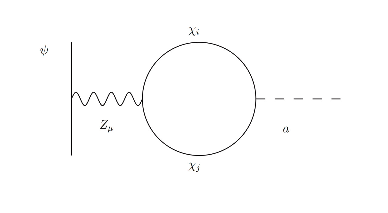
At the one-loop level, a coupling of the PNGB to two electrons is induced by diagrams mediated by the W and the Z bosons [60]. The Z-mediated diagram depicted in Fig. 3 induces the followng terms in the Lagrangian [61]
| (B.3) |
where is any fermion coupling to the boson, and its mass and third component of weak isospin. The loop function is given by
| (B.4) |
where the sum runs over all pairs of charginos and neutralinos with masses and , and is the cutoff of the effective field theory, which we identify with . The coefficients and are given by and , where and are the couplings of the charginos and neutralinos to the Z boson and PNGB, respectively:
| (B.5) |
The coefficients (resp. ) are obtained by diagonalizing the chargino and neutralino mass matrices and writing the boson couplings to leptons, higgsinos and charged wino (resp. the PNGB couplings to fermions (B.2)) in terms of the mass eigenstates ( or ).
Let us now focus on the coupling of the PNGB to electrons. Assuming and , we obtain from Eq. (B.3); the contribution of the W diagram is expected to be of the same order of magnitude. Using the dictionary , we can see from Fig. 4 of Ref. [58] that an axion-like particle with is subject to constraints from red giant cooling and from Edelweiss. The most stringent bound is the red giant one, ( C.L.) [40] (a stronger prelimineray limit, ( C.L.), has been given in Ref. [62]). However, these constraints do not apply if . The Borexino limit shown on the same figure, which is valid for , assumes a specific axion model. One should consider instead the model-independent Borexino constraint ( C.L.) [63], where is the so-called isovector axion-nucleon coupling. Since quarks are not charged under the symmetry of Section 3, and arise at the one-loop level, thus significantly weakening the constraint on 1515 15 One can estimate (where is the nucleon mass), from which the Borexino limit on can be converted into the approximate upper bound .. Furthermore, this bound does not apply for .
In summary, the mass of the PNGB associated with the symmetry of Section 3 is constrained to be larger than about by cosmology, astrophysics and beam dump experiments.
References
- [1] P. Minkowski, Phys. Lett. B 67 (1977), 421-428.
- [2] M. Gell-Mann, P. Ramond and R. Slansky, in Supergravity: Proceedings of the Supergravity Workshop at Stony Brook, Conf. Proc. C 790927 (1979), 315-321 [arXiv:1306.4669 [hep-th]].
- [3] T. Yanagida, in Proceedings of the Workshop on the Baryon Number of the Universe and Unified Theories (Tsukuba, Japan), Conf. Proc. C 7902131 (1979), 95-99.
- [4] F. F. Deppisch, P. Bhupal Dev and A. Pilaftsis, New J. Phys. 17 (2015) no.7, 075019 [arXiv:1502.06541 [hep-ph]].
- [5] Y. Cai, T. Han, T. Li and R. Ruiz, Front. in Phys. 6 (2018), 40 [arXiv:1711.02180 [hep-ph]].
- [6] W. Y. Keung and G. Senjanovic, Phys. Rev. Lett. 50 (1983), 1427.
- [7] P. Abreu et al. [DELPHI], Z. Phys. C 74 (1997), 57-71 [Erratum: Z. Phys. C 75 (1997), 580].
- [8] P. Bamert, C. P. Burgess and R. N. Mohapatra, Nucl. Phys. B 438 (1995), 3-16 [arXiv:hep-ph/9408367 [hep-ph]].
- [9] A. Faessler, M. González, S. Kovalenko and F. Šimkovic, Phys. Rev. D 90 (2014) no.9, 096010 [arXiv:1408.6077 [hep-ph]].
- [10] A. Datta, M. Guchait and A. Pilaftsis, Phys. Rev. D 50 (1994), 3195-3203 [arXiv:hep-ph/9311257 [hep-ph]].
- [11] A. Pilaftsis, Z. Phys. C 55 (1992), 275-282 [arXiv:hep-ph/9901206 [hep-ph]].
- [12] G. Aad et al. [ATLAS], JHEP 07 (2015), 162 [arXiv:1506.06020 [hep-ex]].
- [13] V. Khachatryan et al. [CMS], Phys. Lett. B 748 (2015), 144-166 [arXiv:1501.05566 [hep-ex]].
- [14] V. Khachatryan et al. [CMS], JHEP 04 (2016), 169 [arXiv:1603.02248 [hep-ex]].
- [15] A. M. Sirunyan et al. [CMS], Phys. Rev. Lett. 120, no.22, 221801 (2018) [arXiv:1802.02965 [hep-ex]].
- [16] G. Aad et al. [ATLAS], JHEP 10, 265 (2019) [arXiv:1905.09787 [hep-ex]].
- [17] J. C. Helo, M. Hirsch and S. Kovalenko, Phys. Rev. D 89 (2014), 073005 [arXiv:1312.2900 [hep-ph]].
- [18] E. Izaguirre and B. Shuve, Phys. Rev. D 91, no.9, 093010 (2015) [arXiv:1504.02470 [hep-ph]].
- [19] A. M. Gago, P. Hernández, J. Jones-Pérez, M. Losada and A. Moreno Briceño, Eur. Phys. J. C 75, no.10, 470 (2015) [arXiv:1505.05880 [hep-ph]].
- [20] S. Antusch, E. Cazzato and O. Fischer, Phys. Lett. B 774, 114-118 (2017) [arXiv:1706.05990 [hep-ph]].
- [21] G. Cvetič, A. Das and J. Zamora-Saá, J. Phys. G 46, 075002 (2019) [arXiv:1805.00070 [hep-ph]].
- [22] G. Cottin, J. C. Helo and M. Hirsch, Phys. Rev. D 98, no.3, 035012 (2018) [arXiv:1806.05191 [hep-ph]].
- [23] A. Abada, N. Bernal, M. Losada and X. Marcano, JHEP 01, 093 (2019) [arXiv:1807.10024 [hep-ph]].
- [24] I. Boiarska, K. Bondarenko, A. Boyarsky, S. Eijima, M. Ovchynnikov, O. Ruchayskiy and I. Timiryasov, [arXiv:1902.04535 [hep-ph]].
- [25] C. O. Dib, C. S. Kim and S. Tapia Araya, Phys. Rev. D 101 (2020) no.3, 035022 [arXiv:1903.04905 [hep-ph]].
- [26] M. Drewes and J. Hajer, JHEP 02 (2020), 070 [arXiv:1903.06100 [hep-ph]].
- [27] J. Liu, Z. Liu, L. T. Wang and X. P. Wang, JHEP 07, 159 (2019) [arXiv:1904.01020 [hep-ph]].
- [28] M. Drewes, A. Giammanco, J. Hajer and M. Lucente, Phys. Rev. D 101, no.5, 055002 (2020) [arXiv:1905.09828 [hep-ph]].
- [29] J. Jones-Pérez, J. Masias and J. D. Ruiz-Álvarez, Eur. Phys. J. C 80 (2020) no.7, 642 [arXiv:1912.08206 [hep-ph]].
- [30] J. Alimena, J. Beacham, M. Borsato, Y. Cheng, X. Cid Vidal, G. Cottin, A. De Roeck, N. Desai, D. Curtin and J. A. Evans, et al. J. Phys. G 47 (2020) no.9, 090501 [arXiv:1903.04497 [hep-ex]].
- [31] F. Deppisch, S. Kulkarni and W. Liu, Phys. Rev. D 100 (2019) no.3, 035005 [arXiv:1905.11889 [hep-ph]].
- [32] A. Das, P. S. B. Dev and N. Okada, Phys. Lett. B 799 (2019), 135052 [arXiv:1906.04132 [hep-ph]].
- [33] C. W. Chiang, G. Cottin, A. Das and S. Mandal, JHEP 12 (2019), 070 [arXiv:1908.09838 [hep-ph]].
- [34] L. Covi and F. Dradi, JCAP 10 (2014), 039 [arXiv:1403.4923 [hep-ph]].
- [35] E. Chun, A. S. Joshipura and A. Smirnov, Phys. Lett. B 357 (1995), 608-615 [arXiv:hep-ph/9505275 [hep-ph]].
- [36] E. J. Chun, A. S. Joshipura and A. Y. Smirnov, Phys. Rev. D 54 (1996), 4654-4661 [arXiv:hep-ph/9507371 [hep-ph]].
- [37] E. J. Chun, Phys. Lett. B 454 (1999), 304-308 [arXiv:hep-ph/9901220 [hep-ph]].
- [38] K. Choi, E. J. Chun and K. Hwang, Phys. Rev. D 64 (2001), 033006 [arXiv:hep-ph/0101026 [hep-ph]].
- [39] F. Wilczek, Phys. Rev. Lett. 49 (1982), 1549-1552.
- [40] N. Viaux, M. Catelan, P. B. Stetson, G. Raffelt, J. Redondo, A. A. R. Valcarce and A. Weiss, Phys. Rev. Lett. 111 (2013), 231301 [arXiv:1311.1669 [astro-ph.SR]].
- [41] L. E. Ibanez and G. G. Ross, Nucl. Phys. B 368 (1992), 3-37.
- [42] C. Cheung, G. Elor and L. J. Hall, Phys. Rev. D 85 (2012), 015008 [arXiv:1104.0692 [hep-ph]].
- [43] T. Banks, Y. Grossman, E. Nardi and Y. Nir, Phys. Rev. D 52 (1995), 5319-5325 [arXiv:hep-ph/9505248 [hep-ph]].
- [44] P. Binetruy, E. Dudas, S. Lavignac and C. A. Savoy, Phys. Lett. B 422 (1998), 171-178 [arXiv:hep-ph/9711517 [hep-ph]].
- [45] I. Esteban, M. C. Gonzalez-Garcia, M. Maltoni, T. Schwetz and A. Zhou, [arXiv:2007.14792 [hep-ph]]; NuFIT 5.0 (2020), www.nu-fit.org.
- [46] P. F. de Salas, D. V. Forero, S. Gariazzo, P. Martínez-Miravé, O. Mena, C. A. Ternes, M. Tórtola and J. W. F. Valle, [arXiv:2006.11237 [hep-ph]].
- [47] H. E. Haber and G. L. Kane, Phys. Rept. 117 (1985), 75-263.
- [48] J. F. Gunion and H. E. Haber, Phys. Rev. D 37 (1988), 2515.
- [49] J. C. Helo, S. Kovalenko and I. Schmidt, Nucl. Phys. B 853 (2011), 80-104 [arXiv:1005.1607 [hep-ph]].
- [50] J. Alwall, R. Frederix, S. Frixione, V. Hirschi, F. Maltoni, O. Mattelaer, H. S. Shao, T. Stelzer, P. Torrielli and M. Zaro, JHEP 07 (2014), 079 [arXiv:1405.0301 [hep-ph]].
- [51] M. Aaboud et al. [ATLAS], Phys. Rev. D 97 (2018) no.5, 052010 [arXiv:1712.08119 [hep-ex]].
- [52] A. M. Sirunyan et al. [CMS], JHEP 03 (2018), 166 [arXiv:1709.05406 [hep-ex]].
- [53] A. Gando et al. [KamLAND-Zen], Phys. Rev. Lett. 117 (2016) no.8, 082503 [arXiv:1605.02889 [hep-ex]].
- [54] B. Fuks, M. Klasen, D. R. Lamprea and M. Rothering, JHEP 10 (2012), 081 [arXiv:1207.2159 [hep-ph]].
- [55] B. Fuks, M. Klasen, D. R. Lamprea and M. Rothering, Eur. Phys. J. C 73 (2013), 2480 [arXiv:1304.0790 [hep-ph]].
- [56] D. Cadamuro and J. Redondo, JCAP 02 (2012), 032 [arXiv:1110.2895 [hep-ph]].
- [57] M. Millea, L. Knox and B. Fields, Phys. Rev. D 92 (2015) no.2, 023010 [arXiv:1501.04097 [astro-ph.CO]].
- [58] M. Bauer, M. Neubert and A. Thamm, JHEP 12 (2017), 044 [arXiv:1708.00443 [hep-ph]].
- [59] B. Bellazzini, C. Csaki, J. Hubisz, J. Shao and P. Tanedo, JHEP 09 (2011), 035 [arXiv:1106.2162 [hep-ph]].
- [60] Y. Chikashige, R. N. Mohapatra and R. D. Peccei, Phys. Lett. B 98 (1981), 265-268.
- [61] J. L. Feng, T. Moroi, H. Murayama and E. Schnapka, Phys. Rev. D 57 (1998), 5875-5892 [arXiv:hep-ph/9709411 [hep-ph]].
- [62] O. Straniero, I. Dominguez, M. Giannotti and A. Mirizzi, [arXiv:1802.10357 [astro-ph.SR]].
- [63] G. Bellini et al. [Borexino], Phys. Rev. D 85 (2012), 092003 [arXiv:1203.6258 [hep-ex]].