The Lyman Continuum Escape Survey: Connecting Time-Dependent [O iii] and [O ii] Line Emission with Lyman Continuum Escape Fraction in Simulations of Galaxy FormationJournal: ApJL
Abstract
Escaping Lyman continuum photons from galaxies likely reionized the intergalactic medium at redshifts . However, the Lyman continuum is not directly observable at these redshifts and secondary indicators of Lyman continuum escape must be used to estimate the budget of ionizing photons. Observationally, at redshifts where the Lyman continuum is observationally accessible, surveys have established that many objects that show appreciable Lyman continuum escape fractions also show enhanced [O iii][O ii] (O32) emission line ratios. Here, we use radiative transfer analyses of cosmological zoom-in simulations of galaxy formation to study the physical connection between and O32. Like the observations, we find that the largest values occur at elevated O and that the combination of high and low O32 is extremely rare. While high and O32 often are observable concurrently, the timescales of the physical origin for the processes are very different. Large O32 values fluctuate on short (1 Myr) timescales during the Wolf-Rayet-powered phase after the formation of star clusters, while channels of low absorption are established over tens of megayears by collections of supernovae. We find that while there is no direct causal relation between and O32, high most often occurs after continuous input from star formation-related feedback events that have corresponding excursions to large O32 emission. These calculations are in agreement with interpretations of observations that large tends to occur when O32 is large, but large O32 does not necessarily imply efficient Lyman continuum escape.
I Introduction
The process of cosmic reionization represents a major challenge for understanding the large-scale evolution of the intergalactic medium (IGM). Reionization completed during the first billion years of cosmic history, as evidenced by the prominent Gunn & Peterson 1965 absorption troughs from neutral hydrogen observed in the spectra of quasars at redshifts (Fan et al. 2001; Fan et al. 2006; Bañados et al. 2018). Given the rapid decline in the abundance of bright quasars over the same epoch, star forming galaxies at high redshift likely produced the Lyman continuum photons required to reionize the IGM (Robertson et al. 2015; Bouwens et al. 2015; Finkelstein et al. 2019). The opacity of the mostly ionized IGM at late times remains high enough to prevent the direct detection of Lyman continuum (LyC) photons much beyond redshift (Madau 1995; Steidel et al. 2001; Inoue et al. 2014). During the reionization epoch, probes of the potential LyC production and escape must rely on secondary observational indicators, such as nebular emission lines from galaxies, that the forthcoming James Webb Space Telescope (JWST) will examine in detail. Motivated by the need to understand the physics behind secondary indicators of LyC escape, this Letter presents radiative transfer calculations in high-resolution hydrodynamical simulations of galaxy formation to study the connection between LyC escape fraction and rest-frame optical emission lines powered by ionizing radiation from massive stars.
Given the importance of understanding how galaxies might reionize the IGM, the search for evidence of escaping LyC photons has been wide-ranging. Searches of nearby galaxies have detected LyC emission in some unsually compact or star-bursting galaxies (Borthakur et al. 2014; Izotov et al. 2016a; Izotov et al. 2016b; Leitherer et al. 2016). Blue-sensitive spectrographs have provided direct spectroscopic evidence for LyC emission (Steidel et al. 2001; Shapley et al. 2006; Steidel et al. 2018), as has ground-based continuum imaging (Iwata et al. 2009; Vanzella et al. 2010; Nestor et al. 2011; Nestor et al. 2013; Mostardi et al. 2013; Grazian et al. 2016; Meštrić et al. 2020). Owing to the need for high-resolution imaging in identifying potential foreground contamination (Vanzella et al. 2012; Mostardi et al. 2015), many recent searches for LyC have focused on redshifts where ultraviolet (UV) filters on Hubble Space Telescope (HST) probe blueward of in the galaxy rest frame. These efforts include our LymAn Continuum Escape Survey (Fletcher et al. 2019, LACES, HST GO-14747;) that has to date focused on observational connections between LyC escape and the ionizing photon production evidenced by nebular line emission in galaxies (Nakajima et al. 2020). These direct searches have been complemented by studies of the association of LyC production with ultraviolet or optical nebular lines (Tang et al. 2019; Du et al. 2020), the correspondence between Lyman- and the ([O iii]5007 + [O iii]4959 )/[O ii]3727 line ratio (O32) (Izotov et al. 2020), and the link between LyC escape, H emission, and the rest-frame UV spectral slope (Yamanaka et al. 2020).
Relating LyC and optical emission lines at high redshift currently requires infrared spectrographs on ground-based large telescopes that can access redshifted rest-frame ultraviolet and optical lines (Nakajima et al. 2016; Nakajima et al. 2018). Studies of the LyC-line emission connection are motivated in part by the analysis by Jaskot & Oey 2013; Nakajima & Ouchi 2014, who suggested that the structure of photoionization regions within a galaxy may induce a connection between and O32. Many galaxies with LyC detections at redshifts do indeed show elevated O32 and combined ([O iii]5007 + [O iii]4959 + [O ii]3727)/H 4861 measure known as R23, but not all strong line emitters display escaping LyC (Naidu et al. 2018; Jaskot et al. 2019; Bassett et al. 2019) and active galactic nuclei may contribute to a portion that do (Smith et al. 2018; Smith et al. 2020).
In this Letter, radiative transfer calculations are applied to simulations of galaxy formation to study how LyC escape and optical line emissions are physically connected. The radiative transfer of LyC photons from galaxies has been examined in cosmological simulations of galaxy formation (Ma et al. 2016; Trebitsch et al. 2017, e.g.,), where feedback from star formation was shown to play an important role in enabling hydrogen ionizing photons to escape into the IGM. Previous studies are extended by additionally examining time-dependent [O iii]and [O ii]line emission, and their relation to the ionizing photon production of newly-formed stars (Katz et al. 2020, see also). We show for the first time that galaxy population statistics of and O32 may be explained by these time-dependent processes.
II Methods
II.1 Cosmological Simulation
Results are based on a radiation-hydrodynamic adaptive mesh refinement Enzo (Bryan et al. 2014) simulation evolved from initial conditions produced as part of the Agora collaboration (Kim et al. 2014). The simulation is run with cosmological parameters , , , , , and , which are taken from the most recent release of the Planck Collaboration et al. 2018. Within a 5 Mpc3 box with a root grid size of 1283, a smaller 625 703.125 1093.75 kpc3 sub grid encompassing the Lagrangian volume of a 10 halo (at ) is refined by a factor of 24 to create an effective grid size resolution of (2048)3 with a dark matter particle mass of 1043 . Inside this smaller “zoom-in” region, grids are allowed to further refine adaptively to up to a factor of 214 more than the root grid dimensions as successive density thresholds are exceeded. At this corresponds to a minimum proper cell width of pc, but typical values are between 11 and 180 proper parsecs within the virial radius of the largest halo at that redshift. The simulation includes 9-species (H i, H ii, He i, He ii, He iii, e-, H2, H, H-) radiatively-driven non-equilibrium chemistry, radiating star particles, and supernovae feedback (Wise et al. 2012) with the same parameters and thresholds described in Barrow 2019.
To facilitate analysis of the time-dependence of emission line trends, the state of the simulation is saved every 368,000 years starting at until , which corresponds to about 3,400 outputs. In the simulation, a major merger ( : ) begins at and concludes at . Therefore, two significant halos of roughly similar mass are available for study from until their merger. The larger halo at the time of merger and their resulting combined halo is henceforth referred to as Halo 0 and the smaller member of the merger will be referred to as Halo 1. At , Halo 1 has almost twice the stellar mass as Halo 0 ( versus ), but subsequently exhibits a slower star formation rate. At , the stellar mass and total mass of Halo 0 grows to and respectively.
II.2 Emission Line Model
Emission lines are calculated in roughly the same manner as in Barrow 2019, with some small improvements and additions. To summarize, a halo merger tree is produced by performing an iterative overdensity-finding algorithm tuned to return a consistent halo position and radius between timesteps as well as track Halo 1 through its merger. Then, using Flexible Stellar Population Synthesis (Conroy & Gunn 2010, FSPS;), 8000-wavelength spectra are attached to each star particle based on its age, metallicity isochrome, and mass at each timestep.
From these spectra, a mean galactic spectrum is estimated and combined with the mean metallicity and density of the halo to produce wavelength-dependent absorption cross sections for the gas at 200 temperatures between 102.5 to 107 K using the Cloudy photoionization solver (Ferland et al. 2017). These look up tables are separately generated for each halo and timestep and are attached to the combined mass of absorbers from simulation cells (H i, He i, He ii, H2, H, H-, and metals) as well as the cell temperature along rays to estimate the spectra and flux distribution within the halo. In a test, analytic models for the ionization cross sections of H i, He i, and He ii attached to the corresponding densities from the simulation for comparison. Therein, absorption along rays were roughly equivalent (within 5%) to the Cloudy-generated model at low to moderately high ionization fractions and a bit less absorptive at very high ionization fractions as the importance of H i diminishes and other processes and species dominate the cross section. Because the cross section is only attached to the strong absorbers in the simulation and the cross sections are generated in the presence of the current galactic spectra, much of the non-equilibrium state of the simulation is preserved with this method, while additionally accounting for absorption phenomena that are not explicitly treated in the simulation.
Armed with a model for the attenuated spectra and flux at every point in a halo, a second round of Cloudy calculations are used with a geometry prescription that matches the volume distribution of the flux within each cell to carefully account for the presence of multiple stellar sources as discussed in Barrow 2019, and the resulting emission line luminosities are saved and reported. The prior study used a fixed photon path length to cell width ratio at this stage, whereas the cell photon path length used for the purposes of this calculation is estimated to be the luminosity-weighted mean path length from the stars through the cell to a point with low (1st%ile) flux within the cell. Accordingly, the effective path length may be smaller than the smallest dimension of the cell up to the times the width of the cell depending on the distribution of stars with respect to the cell as well as their luminosity.
II.3 Escape Fraction and Dust Accounting

This work describes the relationship between O32 and the escape fraction of ionizing radiation, , which can be absorbed by both gas and galactic dust. The absorption cross sections used to attenuate stellar light for the emission line model include dust grain extinction, which is implicitly connected to the hydrogen nucleon column density through the use of the mean galactic metallicity in their determination. In this approximation, is calculated as
| (1) |
where is the spectral luminosity of star at frequency in units of erg s-1 Hz-1, is the frequency of the Lyman limit, and the optical depth, , is defined as
| (2) |
where is the summed density of strong absorbers at position and is the temperature-dependent mass attenuation coefficient at position as well as frequency . Eq. 2 is a linear path integral from the position of each star particle, , to a point on the surface of a sphere defined by the virial radius of the halo, , along a vector drawn from one of 972 Hierarchical Equal Area isoLatitude Pixelations (HEALPix) (Górski et al. 2005) of a sphere. Thus, is a projection of onto the virial sphere in each HEALPix direction, simulating parallel rays to an observer from each light source, but not accounting for emission and absorption outside of the virial radius. Depending on the direction, varies wildly owing to the non-homogeneous nature of optical depths among paths through simulated galaxies. While our calculation of escape fraction employs ray tracing at the best resolution available to the simulation, there is some evidence that further resolving cloud structures might affect the morphology of H ii regions immediately after star formation (Geen et al. 2015, e.g.) and further investigations are needed to determine how this might affect galaxy escape fractions.

Because [O iii]5007 and 4959 are at longer wavelengths than the [O ii]3727 doublet and UV/optical dust extinction decreases as a function of wavelength, the presence of dust can increase O32 at the virial radius relative to its intrinsic value in H ii regions. The boost in the ratio between lines at a wavelength A and a wavelength B due solely to dust extinction can be modeled as . If one assumes a similar path length from line emitting regions that produce line A and line B to the virial radius, in terms of the dust column mass density, in g cm-2, and the mass attenuation coefficients, , the boost is . Using the relationship between neutral hydrogen nucleon column density, , and dust column mass density described in Draine 2011, the luminosity-weighted maximum value of in either halo during the course of the simulation from sources to the virial radius among any of the HEALPix directions is
| (3) |
where is the mass of hydrogen and assuming a solar abundance of oxygen. Among the Draine 2003 =3.1, 4.0 and 5.5 dust models, which span the gamut of dust grain compositions and sizes, the maximum value of is . This yields a maximum value of of 1.025, or a 2.5% percent boost. Because this calculation neglects dust scattering, which would further lower the boost by returning a fraction of scattered photons back to the line of sight, and also neglects evidence that lower metallicity galaxies like the halos at in this study have lower dust to ratios (Rémy-Ruyer et al. 2014; Kahre et al. 2018, e.g.), the dust correction to the intrinsic O32 is likely functionally negligible and certainly less than 2.5%. Therefore, only intrinsic O32 values are reported in this study. The same argument applies to R23, since H is also optically thin and of intermediate wavelength between [O ii]3727 and [O iii]4959.
Fig. 1 visually summarizes the data products from the pipeline during a key point in time where Halo 0 exhibits low O32 and high ionizing continuum escape fraction, which is further explored and described in the results section.
II.4 Toy Cluster Model
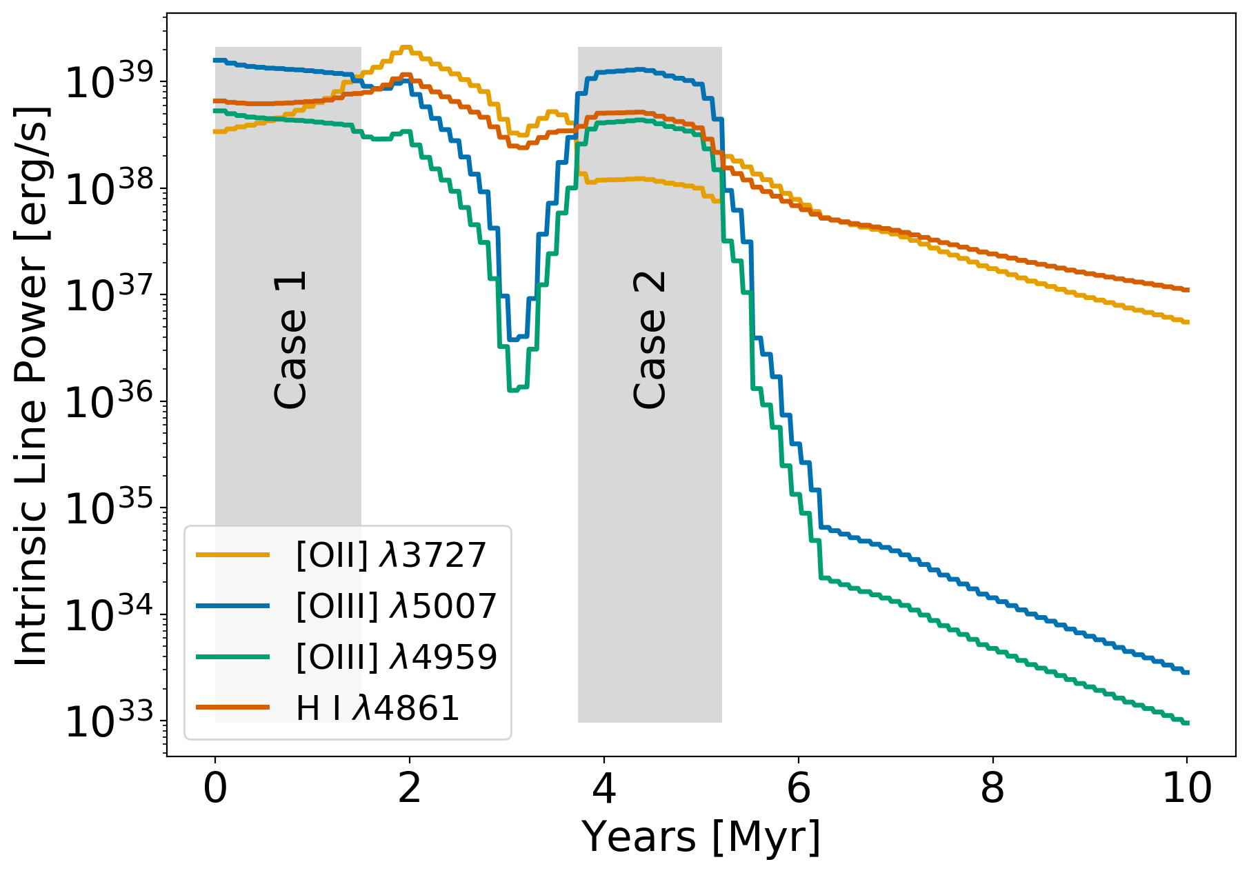
Since the emission lines derived from the simulation exist within a rapidly evolving cosmological environment, a toy model is also devised to clarify trends that exist within star clusters independently of galaxy dynamics. Using just an FSPS model, Cloudy, and a Lamers et al. 2005 cluster mass evolution prescription, trends in [O iii]and [O ii]are computed and plotted in Fig. 2 (see caption for more details).
At the onset of star formation, O32 peaks above one since the [O iii] emission peaks 1.5 Myr before the initial peak in [O ii] emission. In the range of (3.7-5.2 Myr) after the cluster forms, a second, stronger O32 peak occurs because the strength of the [O ii]3727 doublet decays over the first few million years after a star formation event and the harder spectra from the Wolf-Rayet phase of stars in the cluster suddenly converts the reservoir of [O ii]to [O iii].
Since oxygen coincidentally has almost the same ionization energy as hydrogen, [O ii]3727 emission mirrors the evolution of the declining volume of the H ii region and thus closely matches the evolution and strength of H emission except during the Wolf-Rayet phase, where [O ii]3727 is further suppressed. These effects produce two classes of incidents of high O32 ratios: Case 1 ( 1.5 Myr) where [O ii]3727 doublet emission is strong and more likely to be detected, and Case 2 (3.7-5.2 Myr) where [O ii]3727 doublet emission is relatively weak and therefore less likely to be detected. In the interval between the cases, O32 shortly falls to order unity before dipping further.
This toy model only calculates the contribution from a single instantaneous burst, but the broader simulation displays a tendency towards extended star formation events over tens of millions of years (see Fig. 3, bottom plot showing specific star formation rates). Since several star particles are often formed in close spatial and temporal proximity in the simulation, each star formation event results in different emission line signatures due to the overlapping spectral phases of the contributing star particles during their evolution. The size and nature of their encompassing H ii regions may also play a role, which in turn may depend on prior star formation episodes. Therefore, the exercise of classifying O32 peaks in a galactic context is most appropriate in the case of isolated bursty star formation events or isolated star-forming regions and otherwise falls to degeneracies and stochastic peaks. It should also be noted that the existence of these cases is sensitive to the spectra assumptions of FSPS and the earliest few million years after a cluster forms is a challenging modeling problem (Senchyna et al. 2020, e.g.).
III Results
Armed with a generalized radiative transfer model for the production of emission lines within a high-resolution, cosmological simulation of a observably large galaxy, the trends in O32, R23 escape fraction, and metallicity are described in the time domain to theoretically untangle observed correlations in high-redshift, high escape fraction galaxies.
III.1 Time-Dependent Trends
The topmost plot of Fig. 3 displays the evolution of Halo 0 with respect to maximum , O32, and R23 and provides context for the time dependence of the relevant phenomena. Each star formation incident is proceeded by an initial short-lived peak in O32 (Case 1), and followed by a subsequent stronger O32 peak (Case 2) as the spectra hardens during the Wolf-Rayet-powered phase of the star clusters. Bursts of star formation generate stellar and supernovae feedback that tempers subsequent star formation by photo-ionizing the ISM. Thus, high maximum values are rarely coincident with high O32 as the former are tied to minima of the star formation burst cycle. This pattern is repeated in Halo 1 and is not dissimilar from patterns in Ma et al. 2020.
As shown the bottom plot of Fig. 3, halo gas metallicity does not monotonically grow with stellar mass as low-metallicity gas inflows compete with enrichment from stellar feedback. The downward discontinuity in gas metallicity at 1470 Myr is an artifact of the redefinition of Halo 0 to include the merging, lower-metallicity Halo 1 and serves as a marker for the beginning of the merger process. During the merger, the galaxies make four relative periapsides with respect to each other before their bulges merge. Each periapsis drives a long, sustained episode of high star formation rates in both halos. This contrasts with the more sporadic bursts of star formation until the merger event and represents a distinctly dissimilar galactic environment to the pre-merger halos.
Gas mass fraction is physically connected to the escape fraction of ionizing radiation because it modulates the ionizing radiation density needed to create ionized channels through the halo. Low gas mass fractions are also correlated to low neutral hydrogen column densities (shown during the merger as a function of azimuthal and polar angle about the halo in the bottom left plot of Fig. 1) and the peak and minimum column densities decrease by about one order of magnitude between and . Halo 0’s gas mass fraction within its virial radius declines from a high value of at the beginning of the window down to at the end of the window and then further declines to at . At , reaches its highest values, though highly anisotropically, as high star formation rates feed ionizing radiation into a depleted reservoir of gas. In the 345 Myr interval between and , no star formation occurs and the decrease the gas mass fraction is explained by the gas-poor accumulation of dark matter into the halo from the remnants of the merger environment.
III.2 Relationship Between and O32


In Fig. 3, there is a clear offset between the short period bursts of O32 and the longer period peaks of , however a positive correlation between observed and O32 has been described in the literature. In this section, observations in the literature are detailed and then compared to synthetic observations calculated from the simulation to determine whether observed trends can be explained by time-dependent phenomena.
Fig. 4 shows observationally-inferred trends between and (blue and red lines) (Faisst 2016; Izotov et al. 2018). In addition to galaxies that fall within these trends, there exists examples of galaxies with low and high O32 such as J1011+1947, which has an O and or depending on the estimation method, or J1248+4259, which has an O and (Izotov et al. 2018). Recently, Bassett et al. 2019 added a single example (ID: 17251) of low O32 (0.37) and high (0.25) at to the literature and challenged the notion that there is a trend between the two variables at all. These off-trend observations are indicated as red stars in Fig. 4.
In the simulations of Halo 0 and Halo 1, observations of are both time-dependent and galaxy orientation-dependent as high values only escape into the IGM in highly focused channels (as shown in the bottom left plot of Fig. 1), resulting in a distribution of possible observations at each time step. As described in Section II.3, to compute this distribution, O32 values at each timestep are associated with 972 corresponding values in each of the HEALPix directions, resulting in more than two million possible combinations for Halo 0 between and . Combinations of mock observations of O32 and are then histogrammed by fractional occurrence and shown in gray scale in Fig. 4.
III.2.1 Outlying Combinations of O32 and
The resulting simulated distribution roughly traces the distribution of observations including an outlying set of low O32 ( 2) and high () values similar to the outlying observation of 17251 from Bassett et al. 2019. Here we explore why this is rarely observed and falls outside the distribution of the rest of both the simulated and observed data.
Halo 0’s examples of low O32 (0.34) and high ( 0.24) occur at a single timestep of the 3,400 studied (t = 1066.39 Myr, M⋆ = 107.36 M⊙), which can be seen in the top plot of Fig. 3, Fig. 1, and Fig. 4. This instance is about 5.5 Myr after the 5 Myr-averaged specific star formation rate of the halo reaches its highest value over the interval at 42.22 Gyr-1 (30.51 Gyr-1 when averaged over 10 Myr), which corresponds to the end of the Case 2 phase of the O32 emission pattern. At time Myr, [O iii] and [O ii] emission line luminosities are falling rapidly and O32 is itself falling at a rate of about one order of magnitude every 368 kyr timestep. This decline follows several consecutive bursts of rapid star formation, when the distribution of gas in the galaxy is morphologically irregular (as seen in the true-color photon Monte Carlo image in the top left of Fig. 1). Gaps in the gas open in the wake of strong supernovae feedback from prior star formation events, and enable both an abnormally large H ii region and a wide, ionized channel to the virial radius.
The highest escape fraction () in Halo 1 registered when O32 2, but this occurs shortly before the first infall of the merger at and may not be independent of the interaction with Halo 0. That incident is, however, also preceded by a 30 Myr period of sustained star formation with peaks in 5 Myr-averaged specific star formation rates in excess of 15 Gyr-1 that disrupt and precondition the gas for the formation of a larger H ii region.
With sustained star formation, the minimum in O32 between the Case 1 and Case 2 phases is boosted by the constructive sum of stars in various phases of their evolution. Though most star formation events produce multiple star particles in our simulation, real clusters would likely have an even wider range of stellar ages that would further boost the O32 minima between Case 1 and 2. Therefore, the drop in O32 at end of the last Case 2 phase, which occurs at the end of a period of sustained star formation, presents the best opportunity for high with low O32 to be observed. However, that combination of conditions is several times rarer and more transient than other cases where O32 and/or can be observed. In the case of Halo 0, the combination of a large specific star formation rate after a long period of sustained star formation in an irregular and small galaxy suggests that the necessary conditions to produce low O32 and high were not impossibly rare though.
From until , less than one in one hundred thousand synthetic observations of Halo 0 or Halo 1 had a low (0.01-2) O32 and high (0.1) . However, more than one in three hundred combinations of high (0.1) and low to nonexistent (0.01) O32 occurred. These fractions do not correspond to observational probabilities since they do not take into account telescope sensitivity limits and come from a limited sample of galaxies, but do elucidate trends that provide context to the current array of observations. Taken together, the top left region of Fig. 4 (low O32 and high ) is almost completely depopulated for three reasons: 1) the phase offset between high and the presence of O32 due to feedback cycles, 2) the beaming of through ionized channels reducing the overall probability of high observations, and 3) the rarity of cases of low O32 due to it being a more transient state than non-existent or high O32. Conversely, in rare exceptions, outlier values in this region can be produced when conditions align. It should be noted that neither halo explores the full parameter space of observations or conditions as evidenced by the absence of incidences of higher like those reported in (Nakajima et al. 2020) in Fig. 4. A larger sample of simulated galaxies would be needed to make more general inferences about the observed rates.
Importantly, since O32 emission is optically thin and is anisotropic, there is between O32 and in the simulations, despite the trend in observations. Each incident of O32 emission corresponds to a range of possible depending on the observer’s orientation with respect to the galaxy and peaks occur on a longer timescale after star formation than an O32 peak.
III.3 Relationship Between O32, R23, and Metallicity
Under the assumption of solar abundances, Halo 0 non-monotonically traverses a 12 + Log10 [O/H] gas metallicity range from 7.10 to 7.77 over the stellar mass range of 6.92 Log [M⋆/M⊙] 8.31 as it evolves from to . Compared to the sample of lower mass local galaxies from the Andrews & Martini 2013 SDSS metallicity-mass relationship, metallicities in this much higher redshift simulation scatter above and below the mean of the observed trend with a bias towards lower metallicities, especially at higher stellar masses.
The line ratio R23 is often used to estimate the metallicity of observed galaxies. Recently, data collected for high redshift () high EW [O iii] sources showed they occupy a range of R (Nakajima et al. 2020), as plotted with error bars in red on Fig. 5. Some of the lowest R23 ratios are lower bounds due to H and their true R23 may be larger. Similarly, the lower bounds in O32 plotted in Fig. 5 could be significantly less than the true value owing to the presence of [O ii]3727 in the denominator.
To compare with the observations, synthetic R23 and O32 data from Halo 0 are shown in Fig. 5, and colored by metallicity. The simulated galaxies at have lower metallicities than many of the systems in the Nakajima et al. 2020 sample, and both Halo 0 and Halo 1 (not shown) are offset to lower R23 given their lower metallicities. The distribution of O32 vs. R23 values during the evolution of the simulated galaxies is more complicated, and properties beyond metallicity influence its behavior. While the highest O32 values in Halo 0 occurred at low metallicities and low R23, Halo 1 displayed coincident peaks in O32 and R23 during its evolution. This difference suggests that where the maximum of O32 occurs relative to R23 is also connected to, e.g., a galaxy’s specific star formation rate in addition to metallicity. For instance, during individual starbursts when there is a highly variable specific star formation rate, the O32 and R23 line ratios can rapidly move between low O32-low R23 and high O32-high R23 states, and can even show R for short intervals. However, scatter in O32 gradually decreases with increasing gas metallicity.
In summary, while our simulation reproduces many of the LACES observations of R23 and O32, R23 analysis suggests that a higher gas metallicity simulated sample would be needed to cover the full range. Additionally, there is only weak evidence from our simulation that O32 and R23 or O32 and gas metallicity are clearly correlated in this metallicity regime and significant and time-dependent and metallicity-dependent scatter in those relationships exists due to other processes. However, as also seen observations (Maiolino & Mannucci 2019, e.g.), maximum values of O32 decrease with increasing metallicity and R23. While that relationship might help guide comparisons between the work and higher metallicity observations, the scatter inherent in our synthetic line ratio calculations makes those comparisons challenging.
IV Discussion and Conclusions
Using high-resolution zoom-in simulations of star-forming galaxies at , a radiative transfer post-processing is used to explore the time evolution of the emission line ratios O32 and R23, and the Lyman-continuum escape fraction . In summary, our key findings are:
- •
The simulations predict that high escape fraction (e.g., ) is almost always accompanied by high oxygen emission line ratios (e.g., O). However, while and O32 are both powered by a hard ionizing spectra, the response time for the creation of an ionized channel that allows for high is much longer than the production of a high value of O32, and thus the two phenomena are not causally related.
- •
The combination of a low value of O32 and a high is likely a rare event that occurs at the end of a long burst of star formation and persists for only a few hundred thousand years.
- •
Metallicity is degenerate on an O32 versus R23 plot due to tendency for the galaxy to move diagonally through the plane during star formation events.
Though this study was also able to explore more of the galaxy-scale dynamical nebular emission line parameter space than prior studies, our sample galaxies only occupy a portion of the observational space. A complementary recent study explored the statistics of these quantities in static outputs of multi-galaxy simulations (Katz et al. 2020), and the results are broadly consistent despite this studies focus on examining a the time-evolution of only a pair galaxies. Given the importance of the relative time evolution of and O32, a larger sample of simulated galaxies with sufficient time cadence to make statistical arguments about the nature and evolution of nebular emission lines is still required and will be explored in future work.
ACKNOWLEDGMENTS
This work was supported by XSEDE computing grants TG-AST190001 and TG-AST180052 and the Stampede2 supercomputer at the Texas Advanced Computing Center. KSSB was supported by a Porat Postdoctoral Fellowship at Stanford University. BER was supported in part by NASA program HST-GO-14747, contract NNG16PJ25C, and grant 80NSSC18K0563, and NSF award 1828315. RSE and AS acknowledge funding from the European Research Council under the European Union Horizon 2020 research and innovation programme (grant agreement No 669253). We acknowledge use of the lux supercomputer at UC Santa Cruz, funded by NSF MRI grant AST 1828315.
References
- Andrews & Martini (2013) Andrews, B. H., & Martini, P. 2013, ApJ, 765, 140, doi: 10.1088/0004-637X/765/2/140
- Bañados et al. (2018) Bañados, E., Venemans, B. P., Mazzucchelli, C., et al. 2018, Nature, 553, 473, doi: 10.1038/nature25180
- Barrow (2019) Barrow, K. S. S. 2019, MNRAS, 2947, doi: 10.1093/mnras/stz3290
- Bassett et al. (2019) Bassett, R., Ryan-Weber, E. V., Cooke, J., et al. 2019, MNRAS, 483, 5223, doi: 10.1093/mnras/sty3320
- Borthakur et al. (2014) Borthakur, S., Heckman, T. M., Leitherer, C., & Overzier, R. A. 2014, Science, 346, 216, doi: 10.1126/science.1254214
- Bouwens et al. (2015) Bouwens, R. J., Illingworth, G. D., Oesch, P. A., et al. 2015, ApJ, 811, 140, doi: 10.1088/0004-637X/811/2/140
- Bryan et al. (2014) Bryan, G. L., Norman, M. L., O’Shea, B. W., et al. 2014, ApJS, 211, 19, doi: 10.1088/0067-0049/211/2/19
- Conroy & Gunn (2010) Conroy, C., & Gunn, J. E. 2010, ApJ, 712, 833, doi: 10.1088/0004-637X/712/2/833
- Draine (2003) Draine, B. T. 2003, ARA&A, 41, 241, doi: 10.1146/annurev.astro.41.011802.094840
- Draine (2011) Draine, B. T. 2011, Physics of the Interstellar and Intergalactic Medium by Bruce T. Draine. Princeton University Press, 2011. ISBN: 978-0-691-12214-4
- Du et al. (2020) Du, X., Shapley, A. E., Tang, M., et al. 2020, ApJ, 890, 65, doi: 10.3847/1538-4357/ab67b8
- Faisst (2016) Faisst, A. L. 2016, ApJ, 829, 99, doi: 10.3847/0004-637X/829/2/99
- Fan et al. (2001) Fan, X., Narayanan, V. K., Lupton, R. H., et al. 2001, AJ, 122, 2833, doi: 10.1086/324111
- Fan et al. (2006) Fan, X., Strauss, M. A., Becker, R. H., et al. 2006, AJ, 132, 117, doi: 10.1086/504836
- Ferland et al. (2017) Ferland, G. J., Chatzikos, M., Guzmán, F., et al. 2017, Rev. Mexicana Astron. Astrofis., 53, 385. https://arxiv.org/abs/1705.10877
- Finkelstein et al. (2019) Finkelstein, S. L., D’Aloisio, A., Paardekooper, J.-P., et al. 2019, ApJ, 879, 36, doi: 10.3847/1538-4357/ab1ea8
- Fletcher et al. (2019) Fletcher, T. J., Tang, M., Robertson, B. E., et al. 2019, ApJ, 878, 87, doi: 10.3847/1538-4357/ab2045
- Geen et al. (2015) Geen, S., Hennebelle, P., Tremblin, P., & Rosdahl, J. 2015, MNRAS, 454, 4484, doi: 10.1093/mnras/stv2272
- Górski et al. (2005) Górski, K. M., Hivon, E., Banday, A. J., et al. 2005, ApJ, 622, 759, doi: 10.1086/427976
- Grazian et al. (2016) Grazian, A., Giallongo, E., Gerbasi, R., et al. 2016, A&A, 585, A48, doi: 10.1051/0004-6361/201526396
- Gunn & Peterson (1965) Gunn, J. E., & Peterson, B. A. 1965, ApJ, 142, 1633, doi: 10.1086/148444
- Inoue et al. (2014) Inoue, A. K., Shimizu, I., Iwata, I., & Tanaka, M. 2014, MNRAS, 442, 1805, doi: 10.1093/mnras/stu936
- Iwata et al. (2009) Iwata, I., Inoue, A. K., Matsuda, Y., et al. 2009, ApJ, 692, 1287, doi: 10.1088/0004-637X/692/2/1287
- Izotov et al. (2016a) Izotov, Y. I., Orlitová, I., Schaerer, D., et al. 2016a, Nature, 529, 178, doi: 10.1038/nature16456
- Izotov et al. (2016b) Izotov, Y. I., Schaerer, D., Thuan, T. X., et al. 2016b, MNRAS, 461, 3683, doi: 10.1093/mnras/stw1205
- Izotov et al. (2020) Izotov, Y. I., Schaerer, D., Worseck, G., et al. 2020, MNRAS, 491, 468, doi: 10.1093/mnras/stz3041
- Izotov et al. (2018) Izotov, Y. I., Worseck, G., Schaerer, D., et al. 2018, Monthly Notices of the Royal Astronomical Society, 478, 4851, doi: 10.1093/mnras/sty1378
- Jaskot et al. (2019) Jaskot, A. E., Dowd, T., Oey, M. S., Scarlata, C., & McKinney, J. 2019, ApJ, 885, 96, doi: 10.3847/1538-4357/ab3d3b
- Jaskot & Oey (2013) Jaskot, A. E., & Oey, M. S. 2013, ApJ, 766, 91, doi: 10.1088/0004-637X/766/2/91
- Kahre et al. (2018) Kahre, L., Walterbos, R. A., Kim, H., et al. 2018, ApJ, 855, 133, doi: 10.3847/1538-4357/aab101
- Katz et al. (2020) Katz, H., Ďurovčíková, D., Kimm, T., et al. 2020, arXiv e-prints, arXiv:2005.01734. https://arxiv.org/abs/2005.01734
- Kim et al. (2014) Kim, J.-h., Abel, T., Agertz, O., et al. 2014, ApJS, 210, 14, doi: 10.1088/0067-0049/210/1/14
- Lamers et al. (2005) Lamers, H. J. G. L. M., Gieles, M., Bastian, N., et al. 2005, A&A, 441, 117, doi: 10.1051/0004-6361:20042241
- Leitherer et al. (2016) Leitherer, C., Hernandez, S., Lee, J. C., & Oey, M. S. 2016, ApJ, 823, 64, doi: 10.3847/0004-637X/823/1/64
- Ma et al. (2016) Ma, X., Hopkins, P. F., Kasen, D., et al. 2016, MNRAS, 459, 3614, doi: 10.1093/mnras/stw941
- Ma et al. (2020) Ma, X., Quataert, E., Wetzel, A., et al. 2020, MNRAS, doi: 10.1093/mnras/staa2404
- Madau (1995) Madau, P. 1995, ApJ, 441, 18, doi: 10.1086/175332
- Maiolino & Mannucci (2019) Maiolino, R., & Mannucci, F. 2019, A&A Rev., 27, 3, doi: 10.1007/s00159-018-0112-2
- Meštrić et al. (2020) Meštrić, U., Ryan-Weber, E. V., Cooke, J., et al. 2020, MNRAS, doi: 10.1093/mnras/staa920
- Mostardi et al. (2013) Mostardi, R. E., Shapley, A. E., Nestor, D. B., et al. 2013, ApJ, 779, 65, doi: 10.1088/0004-637X/779/1/65
- Mostardi et al. (2015) Mostardi, R. E., Shapley, A. E., Steidel, C. C., et al. 2015, ApJ, 810, 107, doi: 10.1088/0004-637X/810/2/107
- Naidu et al. (2018) Naidu, R. P., Forrest, B., Oesch, P. A., Tran, K.-V. H., & Holden, B. P. 2018, MNRAS, 478, 791, doi: 10.1093/mnras/sty961
- Nakajima et al. (2016) Nakajima, K., Ellis, R. S., Iwata, I., et al. 2016, ApJ, 831, L9, doi: 10.3847/2041-8205/831/1/L9
- Nakajima et al. (2020) Nakajima, K., Ellis, R. S., Robertson, B. E., Tang, M., & Stark, D. P. 2020, ApJ, 889, 161, doi: 10.3847/1538-4357/ab6604
- Nakajima et al. (2018) Nakajima, K., Fletcher, T., Ellis, R. S., Robertson, B. E., & Iwata, I. 2018, MNRAS, 477, 2098, doi: 10.1093/mnras/sty750
- Nakajima & Ouchi (2014) Nakajima, K., & Ouchi, M. 2014, MNRAS, 442, 900, doi: 10.1093/mnras/stu902
- Nestor et al. (2013) Nestor, D. B., Shapley, A. E., Kornei, K. A., Steidel, C. C., & Siana, B. 2013, ApJ, 765, 47, doi: 10.1088/0004-637X/765/1/47
- Nestor et al. (2011) Nestor, D. B., Shapley, A. E., Steidel, C. C., & Siana, B. 2011, ApJ, 736, 18, doi: 10.1088/0004-637X/736/1/18
- Planck Collaboration et al. (2018) Planck Collaboration, Aghanim, N., Akrami, Y., et al. 2018, arXiv e-prints, arXiv:1807.06209. https://arxiv.org/abs/1807.06209
- Rémy-Ruyer et al. (2014) Rémy-Ruyer, A., Madden, S. C., Galliano, F., et al. 2014, A&A, 563, A31, doi: 10.1051/0004-6361/201322803
- Robertson et al. (2015) Robertson, B. E., Ellis, R. S., Furlanetto, S. R., & Dunlop, J. S. 2015, ApJ, 802, L19, doi: 10.1088/2041-8205/802/2/L19
- Senchyna et al. (2020) Senchyna, P., Stark, D. P., Charlot, S., et al. 2020, arXiv e-prints, arXiv:2008.09780. https://arxiv.org/abs/2008.09780
- Shapley et al. (2006) Shapley, A. E., Steidel, C. C., Pettini, M., Adelberger, K. L., & Erb, D. K. 2006, ApJ, 651, 688, doi: 10.1086/507511
- Smith et al. (2018) Smith, B. M., Windhorst, R. A., Jansen, R. A., et al. 2018, ApJ, 853, 191, doi: 10.3847/1538-4357/aaa3dc
- Smith et al. (2020) Smith, B. M., Windhorst, R. A., Cohen, S. H., et al. 2020, arXiv e-prints, arXiv:2004.04360. https://arxiv.org/abs/2004.04360
- Steidel et al. (2018) Steidel, C. C., Bogosavljević, M., Shapley, A. E., et al. 2018, ApJ, 869, 123, doi: 10.3847/1538-4357/aaed28
- Steidel et al. (2001) Steidel, C. C., Pettini, M., & Adelberger, K. L. 2001, ApJ, 546, 665, doi: 10.1086/318323
- Tang et al. (2019) Tang, M., Stark, D. P., Chevallard, J., & Charlot, S. 2019, MNRAS, 489, 2572, doi: 10.1093/mnras/stz2236
- Trebitsch et al. (2017) Trebitsch, M., Blaizot, J., Rosdahl, J., Devriendt, J., & Slyz, A. 2017, MNRAS, 470, 224, doi: 10.1093/mnras/stx1060
- Vanzella et al. (2010) Vanzella, E., Giavalisco, M., Inoue, A. K., et al. 2010, ApJ, 725, 1011, doi: 10.1088/0004-637X/725/1/1011
- Vanzella et al. (2012) Vanzella, E., Guo, Y., Giavalisco, M., et al. 2012, ApJ, 751, 70, doi: 10.1088/0004-637X/751/1/70
- Wise et al. (2012) Wise, J. H., Abel, T., Turk, M. J., Norman, M. L., & Smith, B. D. 2012, MNRAS, 427, 311, doi: 10.1111/j.1365-2966.2012.21809.x
- Yamanaka et al. (2020) Yamanaka, S., Inoue, A. K., Yamada, T., et al. 2020, arXiv e-prints, arXiv:2003.03905. https://arxiv.org/abs/2003.03905