A photoionized accretion disk around a young high-mass star.Facilities: ALMACASA (McMullin et al. 2007), Perl Data Language http://pdl.perl.org
Abstract
We present high spatial resolution ( au) observations of the high-mass young stellar object (HMYSO) G345.4938+01.4677 made using the Atacama Large Millimeter/sub-millimeter Array (ALMA). This O-type HMYSO is located at 2.38 kpc and it is associated with a luminosity of . We detect circumstellar emission from the H hydrogen recombination line showing a compact structure rotating perpendicularly to the previously detected radio jet. We interpret this emission as tracing a photo-ionized accretion disk around the HMYSO. While this disk-like structure seems currently too small to sustain continued accretion, the data present direct observational evidence of how disks can effectively survive the photo-ionization feedback from young high-mass stars. We also report the detection of a low-mass young stellar object in the vicinity of the HMYSO and suggest that it forms a high-mass and low-mass star binary system.
I Introduction.
In the recent years, and with the advent of new observational instruments such as the Atacama Large Millimeter/sub-millimeter Array (ALMA), evidence have been gathering pointing toward most high-mass stars acquiring their mass through disk accretion (Tan et al. 2014). It is becoming apparent that the principal characteristic which allows accretion to proceed onto most young high-mass young stellar objects (HMYSOs) — despite the venerable theoretical problems of radiation and ionization feedback (Wolfire & Cassinelli 1987; Kahn 1974; Larson & Starrfield 1971) — is that this accretion occurs through a disk (Kuiper et al. 2010; Yorke & Sonnhalter 2002; Nakano 1989).
The signposts of disk accretion toward embedded HMYSOs are mainly of two kinds: highly collimated (aperture ) fast jets with velocities comparable to the escape speed of the compact object, and compact (sub-1000 au) circumstellar disks. Slower, less collimated outflows can be produced by other processes like ionization feedback (Peters et al. 2012), magnetic braking (Hennebelle et al. 2011), and mergers of smaller stars (Bally & Zinnecker 2005). Rotating structures 3000 au or bigger (Beltrán & de Wit 2016) are too large to link them necessarily with disk accretion onto a central, compact HMYSO, and may even be transient non-equilibrium structures (so-called toroids, Cesaroni et al. 2006).
Examples of HMYSOs in which collimated fast jets and compact sub-1000 au disks are detected simultaneously are GGD 27 (Girart et al. 2017; Masqué et al. 2015) and Cepheus A HW2 (Torrelles et al. 2007; Curiel et al. 2006). In these two HMYSOs, a compact disk is detected in molecular lines and the proper motion of the ionized lobes excited by the underlying jet indicate velocities in excess of 500 km s-1. Additionally, Jiménez-Serra et al. 2011 determined in Cepheus A HW2 the possible presence of high-velocity ionized gas associated with the jet by measuring the width of the associated hydrogen recombination lines (HRLs). Sources G343.12620.0620 (also IRAS165474247, Zapata et al. 2019; Rodríguez et al. 2008) and G35.200.74N (Beltrán et al. 2016; Sánchez-Monge et al. 2013), are also good examples, although the presence of a binary companion somewhat confuses the proper motion signals from the ionized lobes. In all these sources, the determined velocities are in excess of 200 km s-1, which is the approximate escape velocity of a 8 star of radius 100 . This large radius is expected during the early phase of the HMYSO due to the large accretion rates (Zhang et al. 2014), and 200 km s-1 is a rough lower limit on the expected velocities associated with the gas tracing accretion onto the central object. Examples such as IRAS 134816124 (Caratti o Garatti et al. 2016; Boley et al. 2016) and W33A VLA1 (Davies et al. 2010) are less embedded, which allows its study in the infrared (IR). Disks in these sources are detected through near- and mid-IR interferometry (IRAS 134816124) and CO overtone mapping (W33A). The high-velocity ionized gas in these sources traces bipolar geometries as determined using Br spectro-astrometry. In addition, W33A is associated with an ionized jet detected in cm free-free continuum (Sanna et al. 2018). High-velocity ( km s-1) ionized gas is more commonly detected in the near-IR through (inverse) P-Cygni profiles of HRLs, which provides no constraints to the geometry or orientation of the outflow. One noticeable example, G018.3412+01.7681 (IRAS 181511208 B), is associated with an ionized jet (Rosero et al. 2019), a perpendicularly rotating toroid (Beltrán & de Wit 2016), and a Br line displaying a P-Cygni profile (Cooper et al. 2013). Cooper et al. 2013 also present another 20 P-Cygni HMYSOs detected in spectra with 600 km s-1 spectral resolution (suggesting even larger expansion velocities). G094.602801.7966 is another interesting source in which the Br P-Cygni signature is present (Pomohaci et al. 2017) and is associated with non-thermal jet lobes (Obonyo et al. 2019). Eight more HMYSOs associated with P-Cygni profiles are shown in Pomohaci et al. 2017. Finally, we note S255 SMA 1 (also S255 NIRS 3), associated with a molecular disk, a jet, (Cesaroni et al. 2018; Zinchenko et al. 2015), and a high velocity Pa P-Cygni profile reported as a private communication in Cesaroni et al. 2018.
Perhaps not surprisingly, in most cases the high-velocity gas is ionized (Titmarsh et al. 2013, with few exceptions, cf.). Because of the small distances to the HMYSO and the fast shock velocities involved, molecules are likely dissociated. In general, velocities probed by water masers are the highest among those probed by the other molecular outflow tracers. Examples of disk+outflow systems detected in molecular maser transitions, with associated ionized jets, are given in Table 3 of Sanna et al. 2018, to which we add G16.590.05 (Moscadelli et al. 2019; Moscadelli et al. 2013), G353.273+0.641 (Motogi et al. 2013; Motogi et al. 2019), likely W75N(B) VLA 2 (Carrasco-González et al. 2015), and possibly NGC 7538 IRS 1 (although results in Beuther et al. 2017 favor a different interpretation). Finally, pseudo-thermal (as opposed to strong masers) molecular lines have revealed several examples of compact disks and collimated molecular outflows associated with HMYSOs. Among these, noticeable examples are those detected toward AFGL 4176 (Johnston et al. 2015), G11.920.61 MM1 (Ilee et al. 2018; Ilee et al. 2016) G17.64+0.16 (Maud et al. 2019; Maud et al. 2018, also CRL 2136), Orion Src I (Ginsburg et al. 2018; Hirota et al. 2017), G343.12620.0620 (Zapata et al. 2015; Zapata et al. 2019)
All these examples demonstrate that disk accretion plays a role in assembling massive stars, although, what fraction of the mass is accreted in this way is still unclear. Theoretically, disk accretion should be effective after the protostar has contracted and it should allow accretion to proceed until reaching the star’s final mass (Sartorio et al. 2019; Kuiper & Hosokawa 2018; Keto 2007), in spite of the presence of UV radiation and ionized gas. At least for accretion rates yr-1 (Hosokawa et al. 2010), the short Kelvin-Helmholtz timescale in HMYSOs ensures that a large fraction of the mass in O-type stars will be accreted after protostellar contraction. In the simulations by Zhang et al. 2014, for example, they show that an accreting HMYSO reaches surface temperatures K — sufficient to excite an Hii region — when it has accreted , that is, about half of its final mass of 26 .
However, most of the HMYSOs above have no associated Hii region. An ALMA search for compact disks toward HMYSOs with signs of rotation at au scales performed by Cesaroni et al. 2017 suggests that more evolved targets — that is, those associated with hyper-compact (HC) Hii regions — seem to lack a compact molecular disk counterpart when observed with high angular resolution (at least in CH3CN). While the specific reason for disk non-detection may be somewhat related to the selected tracer (e.g. G17.64+0.16, Maud et al. 2018), there are alternative pictures in the literature which do not necessarily require a long-lived disk from where the HMYSO gathers its mass after the HC Hii region stage (Goddi et al. 2018; De Pree et al. 2014).
In this work, we focus on G345.4938+01.4677 (G345.49+1.47 hereafter), a HMYSO located at 2.38 kpc (Lumsden et al. 2013; Mottram et al. 2011; Moisés et al. 2011). G345.49+1.47 is associated with an HC Hii region, a massive molecular outflow (Guzmán et al. 2011), a high-velocity ( km s-1) ionized jet (Guzmán et al. 2016), and a perpendicularly rotating core (Guzmán et al. 2014) of diameter au detected in sulfur oxide lines (SO, SO2 and isotopologues). G345.49+1.47 is part of a small group of HMYSOs toward which active disk accretion has been proposed while simultaneously exciting an Hii region. Other like sources are G35.200.74N (Beltrán et al. 2016) and recently W75N (B) VLA1 (Rodríguez-Kamenetzky et al. 2020). G345.49+1.47 was also part of the sources studied by Cesaroni et al. 2017 at 02 angular resolution.
Here, we present and analyze new high-angular resolution ( mas, equivalent to 52 au) line (H38 HRL) observations of G345.49+1.47 and its adjacent continuum. High angular resolution HRL observations have been used to trace the dynamics (rotation and outflows) of ionized gas around HMYSOs such as IRAS 072991651 (also G232.6207+00.9959, Zhang et al. 2019a), G45.47+0.05 (Zhang et al. 2019b), and G17.64+0.16 (Maud et al. 2019). Section II presents the observations and describes the data reduction. Observational results are presented in Section III and the main analysis and discussion in Section IV. The main conclusions of this work are summarized in Section V.
II Observations.
Observations of G345.49+1.47 were taken using the ALMA Band 6 in two sessions taken the 8th and 9th of July 2019 (UT). They consisted of 12m-array single pointing (field of view FWHM ) scans toward R.A.=16h59m4163, decl.= (ICRS) in five spectral windows (SpWs) centered at the frequencies of 219.54, 220.41, 220.43, 222.75, and 224.72 GHz and covering 1875, 234.4, 234.4, 1875, and 234.4 MHz, respectively. The bandpass and primary flux calibrators for the 8th and 9th of July sessions were J19242914 and J1427, whose fluxes at 222.75 GHz were fixed at 2.817 and 1.077 Jy, respectively. The absolute flux calibration of ALMA in band 6 is estimated to be accurate within 10% (Remijan et al. 2019).
Table 1 shows some observational parameters of the data: columns (1) to (9) show the ALMA band, the number of antennae employed, the reference frequency, the flux of the phase calibrator J17113744 at the reference frequency, the date of the observations, the on-source time, the approximate maximum angular resolution (MAR, given by , where is the largest baseline), the maximum recoverable scale (MRS, given by , where is the shortest baseline, see Eq. (3.28) in Remijan et al. 2019), and the median measured during the observations.
We focus our analysis on the 1875 MHz wide SpW centered at 222.75 GHz ( mm). This SpW covers the H38 HRL whose rest frequency is 222011.75545 MHz. The velocity width of the channels covering the H38 line is 1.32 km s-1, and the spectral resolution of the data cubes is 2.64 km s-1.
Calibration and reduction of these data were done using the Common Astronomy and Software Applications (McMullin et al. 2007, CASA,) v. 5.4. A priori calibration based on external calibrators was carried out by the ALMA East-Asia regional center. A continuum level was determined from the calibrated uv-data from the line-free channels of the SpW and subtracted using the task uvcontsub. Continuum images of the 1875 MHz SpW were obtained with the task tclean using multi-frequency synthesis and Briggs weighting (Briggs 1995) using robust parameter set to 0. Several iterations of phase self-calibration were applied to the continuum, until reaching a gain calibration solution sampled every 15 s. These gain tables were later applied to the continuum subtracted uv-data, from where image cubes were synthesized following the same procedure and uv-weighting scheme as with the continuum, but channel per channel. The total mapped region in both continuum and line was selected to cover the region where the primary beam response is above 0.2, corresponding to a diameter of around the phase center. Table 2 details some observational characteristics of the final reduced data products. Calibrated images and cubes of the HRL can be found in Guzmán 2020.
| Band | # | Reference | Phase cal. | Observation | MAR⋆ | MRS† | ||
|---|---|---|---|---|---|---|---|---|
| Ant. | frequency | flux | date | |||||
| (GHz) | (mJy) | (dd-mm-yyyy) | (s) | (mas) | (″) | (K) | ||
| 6 | 46 | 222.747 | 116.5 | 08-07-2019 | 2624 | 18.5 | 1.12 | 85 |
| 6 | 44 | 222.747 | 111.4 | 09-07-2017 | 2622 | 19.9 | 1.12 | 75 |
| ‡ Time spent on the science source as reported in the observing log. | ||||||||
| ⋆ Maximum angular resolution, given by . | ||||||||
| † Maximum recoverable scale, given by (Eq. (3.28) in Remijan et al. 2019). | ||||||||
| Image | Spectral | Synth. beam | rms | Dynamic |
|---|---|---|---|---|
| resolution | bmajbmin, pa | range | ||
| (km s-1) | (mas mas, ∘) | (Jy beam-1) | ||
| Continuum | , | 30 | 2300 | |
| H38 cube | 2.64 | , | 696 | 12 |
III Results
Figure 1 shows the continuum and H38 data obtained toward G345.49+1.47. Left panel shows the H38 moment 1 overlaid with continuum levels. As shown by the contours, the spatial distribution of the resolved continuum emission at 222.7617 GHz near G345.49+1.47 matches the distribution of the line, at least over the first contour at mJy beam-1. This indicates that a large fraction of this continuum emission comes from free-free. We fit a 2D Gaussian to the continuum emission using the task imfit within CASA. Table 3 shows the best-fit source parameters. Throughout this work we will use the position of this source as reference whenever offsets are used as spatial axes.
Figure 2 shows the low-brightness continuum emission around G345.49+1.47. We detect emission surrounding the HMYSO protruding in the north-west and south-east directions extending 01, although there is a hint of additional filamentary emission extending toward the south for 025. We integrate the intensity within 03 around G345.49+1.47 and report it in Table 3. While the extended features detected are within the MRS, we emphasize that (by definition) the recovered brightness fraction of a structure homogeneous within the MRS size is approximately equal to or . Hence, part of the emission of the more extended features in Figure 2 likely are being partially filtered.
In addition, we report the detection of unresolved Source 10a (G345.49+1.47 is Source 10 in Guzmán et al. 2014) located 029 to the south-east from G345.49+1.47, or au in projection. The flux density of this source is smaller than the rms in the data presented by Cesaroni et al. 2017, but we are able to detect it with a SNR .
To evaluate whether Source 10a may be part of extragalactic contamination, we extrapolate with a power-law the source counts from the survey of Mocanu et al. 2013 at 220 GHz, obtaining a source density of deg-2 mJy-1. Based on this extrapolation, we estimate extragalactic sources per deg2 as bright as 10a, or sources within the primary beam of our observations. We conclude that Source 10a is Galactic in nature and part of the IRAS 165623959 clump.
| Source | R.A. | Decl. | Flux | Deconvolved size | Integrated |
|---|---|---|---|---|---|
| ICRS | (ICRS) | density | bmaj bmin, P.A. | flux density††Within 03 for G345.49+1.47 and within 50 mas for 10a. | |
| (16h:59m:) | (°:03′:) | (mJy) | (mas mas, °) | (mJy) | |
| G345.49+1.47 | 416264 | 43641 | , | ||
| Source 10a | 416430 | 43853 | unresolved |


The right panel of Figure 1 shows the H38 spectrum integrated in a circle of 50 mas around G345.49+1.47. The HRL is characterized by a width of km s-1, is centered around km s-1, and has a total flux of Jy km s-1. The noise level of this integrated spectrum is mJy. The line flux peaks at mJy beam-1 ( K). The molecular line absorption shown in Figure 1 is due to the SO line centered at MHz. This line has an upper energy level of K (Pickett et al. 1998). We observe emission from this line on a more extended spatial distribution than that of the HRL. The H38 moment 1 map in Figure 1 clearly shows we are able to resolve the H38 emission. This is further illustrated by the position velocity diagram (pv-diagram) of the HRL shown in Figure 3. The position velocity diagram shows the average intensity over one beam width across a P.A. line centered on the position of G345.49+1.47 and has a noise level of 0.51 mJy beam-1. The range used to calculate the moment 1 is , including only emission above and excluding the line wings. This threshold allows us to negate the influence of the SO2 absorption affecting the red-shifted slope of the line. The statistical uncertainty derived of the velocity map ranges between – km s-1, depending somewhat on the number of channels included in the moment 1 calculation for each position. Figure 3 illustrates that most of the HRL emission is not affected by the molecular absorption. We measure a velocity gradient in the P.A. direction of km s-1 mas-1 ( km s-1 au-1 at 2.38 kpc). H38 is not detected toward any other location of the map. The pv-diagram of the HRL somewhat resembles that of H30 in G17.64+0.16 (Maud et al. 2019, their Figure A.1).
IV Discussion
In this section we analyze in more detail the physical interpretation of the HRL and its characteristics. One important physical parameter for this analysis is the distance to G345.49+1.47. For this work, we use the spectrophotometric distance of 2.38 kpc (Moisés et al. 2011) instead of the kinematic distance of 1.7 kpc used by several authors before. Both estimations have appeared in the literature. However, results from Gaia Collaboration et al. 2018; Gaia Collaboration et al. 2016 make the 2.38 kpc distance estimation more plausible taking into account the low extinction levels and 1.82 (Andrae et al. 2018) and the parallax distance estimations of and pc (Luri et al. 2018) determined toward 2MASS sources J165942974003114 and J165939284004080, respectively. These two sources are in the field of the massive molecular clump IRAS 165623959, of which G345.49+1.47 is the central, dominating HMYSO. However, from the 1.2 mm dust emission and the molecular clump model of Guzmán et al. 2010, we derive an H2 column density in the direction of these two sources of about cm-2, which is more than an order of magnitude larger than those derived from the extinction values, suggesting that these two near-IR sources are in the foreground of IRAS 165623959. The appearance of these sources in three-color JHKS images also suggests they are in the foreground, situating G345.49+1.47 farther than 2 kpc.
IV.1 HRL and Continuum Emission
Because both the free-free emission and the HRL arise from the same ionized gas, we can use the H38 line to estimate the free-free contribution to the observed continuum emission. Under LTE conditions, the H38 optical depth is given by , where is defined in Guzmán et al. 2014 and is the line profile. We define the line to continuum equivalent width , where is the free-free opacity. For the the H38 recombination line we have
| (1) |
where the dependance on the temperature is adequate for the frequency of this HRL. From (1), we can derive the LTE ratio between the integrated line flux to the free-free continuum. That is,
| (2) |
where is an opacity correction factor which is unity for optically thin emission and decreases to zero monotonically with increasing . We argue that LTE should be a reasonable approximation in G345.49+1.47 because the electron density is high enough to ensure thermalization via collisions. The thermalization critical density is cm-3 (Strelnitski et al. 1996) for H38, which is lower than the electron density found by Guzmán et al. 2014 at even larger physical scales than the ones probed by this study. Hereafter, we will use K which is adequate for Hii regions located at the Galactocentric distance of G345.49+1.47 (Paladini et al. 2004).
Observationally, the integrated line flux to continuum ratio in G345.49+1.47 is km s-1, which is lower than the value of km s-1 obtained from Equation (1) using K. Because the continuum emission does not seem to follow the power-law — characteristic of partially optically thick free-free emission — determined in Guzmán et al. 2016, it is likely that the free-free emission at 220 GHz from the HC Hii region is already optically thin. Therefore, we propose that the excess continuum emission relative to that inferred from the HRL arises from thermal dust emission. This dust emission contribution is about mJy. Considering that the dust emission estimated by Guzmán et al. 2014 at 92 GHz is mJy, the derived 220 GHz dust emission is consistent with the observed ranges of dust mm spectral indices (Orozco-Aguilera et al. 2017, e.g.,).
IV.2 A Photoionized Disk
We interpret the velocity profile of the H38 line as rotation around the HMYSO G345.49+1.47. In this case, a simple model for the emission is that of a Keplerian disk as used in G17.64+0.16 by Maud et al. 2018. However, we must first note that, when considering only rotation, there is a diameter of the disk whose velocity projected in the line of sight (l.o.s.) is zero. This diameter corresponds to the minor axis of the ellipse projected by the disk in the plane of the sky. That is, emission at the source’s traces a straight line in the velocity moment 1 map. However, as shown in Figure 1, the emission at the source — which separates the blue- and red-shifted halves of the rotating structure — clearly traces a slanted serpentine shape, to which we will refer hereafter as a S -shape.11 1 Alternatively, the moment 1 panels shown in Figure 1 can be described as resembling a taijitu or ying-yang symbol. This S -shape is characteristic of radial motions combined with rotation, specifically, radial motions in which the rotation to radial velocity ratio is not constant with radii. Therefore, in order to reproduce this observed feature, we include radial motions in the disk in addition to rotation. Compared to the pv-diagram analysis of SiO in G17.64+0.16 done by Maud et al. 2018, our G345.49+1.47 pv-diagram (Figure 3) seems to be less informative, possibly due to HRLs being much wider than molecular lines. Therefore, in our case, the main indication of radial motions relies on the aspect of the moment 1 map rather than that of the pv-diagram.
The model consists of a thin circular disk of ionized gas whose position, orientation, and define five free parameters. The rotation is assumed to be Keplerian defined by a central mass, and the radial motion has a constant magnitude. The disk is characterized by a radial electron emission measure (Wilson et al. 2013, EM, Equation (10.34) in ) distribution, truncated at an external radius . The disk also has a width which, in combination with the emission measure, determines the electron density of the disk as
| (3) |
Electron density affects HRLs through pressure or collisional broadening: in general, the shape of an HRL is a Voigt profile, defined as the convolution of a Gaussian with a thermal width and a Lorentz profile with width parameter given by Gordon & Sorochenko 2002. For H38, the Lorentz width parameter is km s-1, where is the electron density in units of cm-3.

Before determining the best fit model, we define some constraints on the orientation of the disk based on previous studies. Let us consider a right hand oriented system of reference where directions are east, north, and the l.o.s., respectively. The orientation and rotation direction of the disk is defined by the direction of its angular momentum . We define the inclination angle of the disk as the angle formed between and . Figure 4 shows schematically the projections of the disk orientation in the adopted reference system. The P.A. and angle are measured in the plane of the sky and in the l.o.s.– plane, respectively (i.e., the inclination of the disk respect to the plane of the sky is ). We will consider models in which the axis of the disk is consistent with the jet direction and rotation shown in Figure 1. This not only means that P.A., but also that the direction corresponds to the blue-shifted half of the jet which is closer to the observer than the western half (Figure 4). This constraint, combined with the observed rotation, implies that points toward us (that is, or ).
These geometric considerations solve the expansion-contraction degeneracy of the radial motions: for G345.49+1.47, the S -shape noted above in the moment 1 map for velocities close to the corresponds to expansion. Contracting motions would create a S-shape pattern instead.
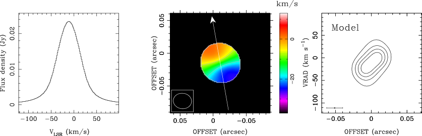
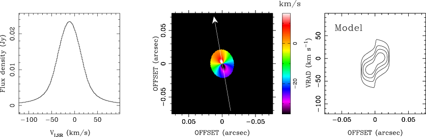
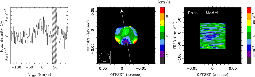
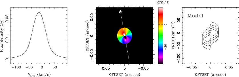
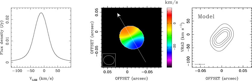
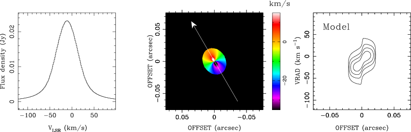
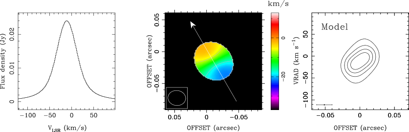
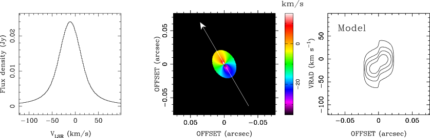
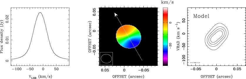
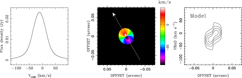
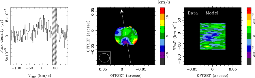
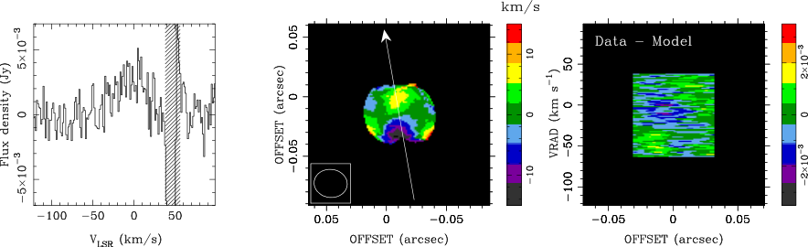
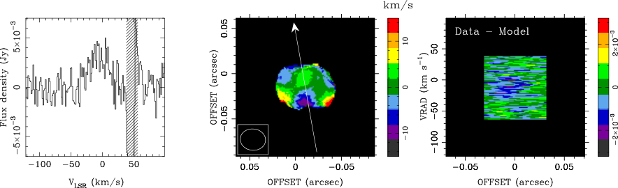
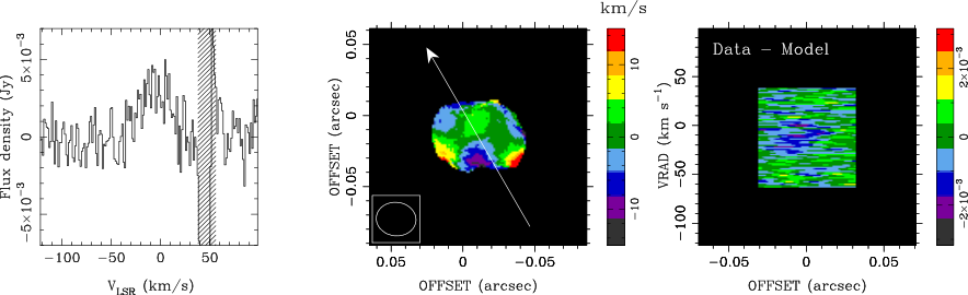
Figure 5 shows the results of the model that best fits the data towards G345.49+1.47. The leftmost column of panels shows the total flux density spectra, the middle column the moment 1 maps, and the rightmost column the position velocity diagrams. The top panel row shows these three diagnostic plots for the observed data. To determine the best-fit model, we calculate the simulated spectrum, moment 1, and pv-diagram and convolved them with the spatial resolution (Richer & Padman 1991). Note that the spectral resolution of the data is very small compared to the width of the line. The convolved models are shown in the second row of panels in Figure 5. The model shown in the first panel of this second row is the same as the one shown in the top-left panel. The third row of plots also show the three diagnostics (spectrum, moment 1, and pv-diagram) of the best-fit model, but not convolved with the beam. We calculate the difference between the convolved model and the data, and minimize the squared difference weighted by the inverse variance of the data. Table 4 shows the best-fit parameters of the disk, together with those parameters which were held fixed. The minimization and errors were calculated using the Minuit package (James & Roos 1975), as implemented in the Perl Data Language. Computational routines can be found in Guzmán 2020. Error bars in Table 4 represent statistical uncertainties.

S
| Parameter | Best-fit value | |
|---|---|---|
| km s-1 | ||
| P.A. | (fixed) | |
| ††footnotemark: | ||
| (fixed) | ||
| ° | ||
| K (fixed) | ||
| au | ||
| km s-1 | ||
| au |
Note. — Using our notation, the inclination of the disk axis respect to the plane of the sky is .
One of the most important parameters of the G345.49+1.47 system is the mass of the HMYSO. This mass is degenerate with the inclination, resulting in higher mass estimations for smaller angles. There are several arguments that limit the possible mass or inclination of the G345.49+1.47 system. From the bolometric luminosity of , we derive that the mass of this HMYSO is using the stellar parameters from Davies et al. 2011. The geometry of the outflow, jet, and outflow cavity also give some clues about the inclination of the disk, under the assumption that the outflow and the disk share the same axis. Guzmán et al. 2016, by comparing the jet lobes’ proper motion velocity with the escape velocity of the star, derived that assuming . In general, for and using this same argument, we obtain . Guzmán et al. 2016 also show the NIR cavity observed toward the blue-shifted side of G345.49+1.47 which has no extension toward the redshifted side of the jet. This indicates that the line of sight toward the HMYSO is not contained by the outflow cavity, and therefore the inclination angle is less than , where is the semi-aperture angle of the cavity.22 2 From the NIR images we cannot derive a lower bound for . The projected aperture angle of the cavity is 45°, that is, . Additionally, the red- and blue-shifted halves of the CO bipolar molecular outflow associated with G345.49+1.47 are well separated (Guzmán et al. 2011), indicating that the outflow is not near the plane of the sky or that is well above . Finally, we emphasize that due to the configuration of the outflow cavity it is possible that the true bolometric luminosity of G345.49+1.47 is larger than that given by Mottram et al. 2011 by a factor of up to 3 due to the flashlight effect (Zhang & Tan 2018). This correction would increase the mass estimate in about a 70%. In Appendix A we present models assuming a HMYSO mass of 56 and 15 to encompass this uncertainty and the masses used also in previous literature (Guzmán et al. 2014, e.g.,). While in each table we provide the statistical error derived from the fitting, the dispersion of best-fit values can give a rough estimation of the systematic uncertainty derived using different assumptions. Specifically for the inclination, the range of HMYSO masses consistent with the luminosity constraints given above is associated with a range of inclinations which span at least around the best-fit value given in Table 4.
Figure 6 shows the difference between the best-fit model and the data. Residuals of the moment 1 map are largest near the blue-shifted peak, while the pv-diagram shows some negative residuals (overestimation of the model) at the level. Note also that whereas the projected elongation of a rotating disk is expected to occur along the highest velocity gradient direction, the H38 emission is more elongated in the perpendicular direction, i.e., along the jet direction. This is possibly due to expansion of the HC Hii region along the polar axis (Section IV.3), which is not included in the model. This component may also produce the excess emission observed in the first panel of Figure 6.
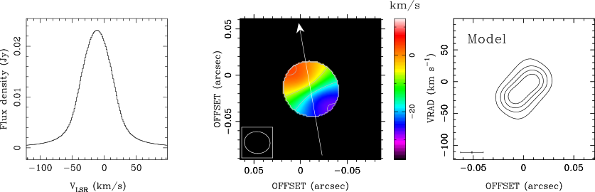
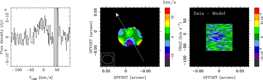
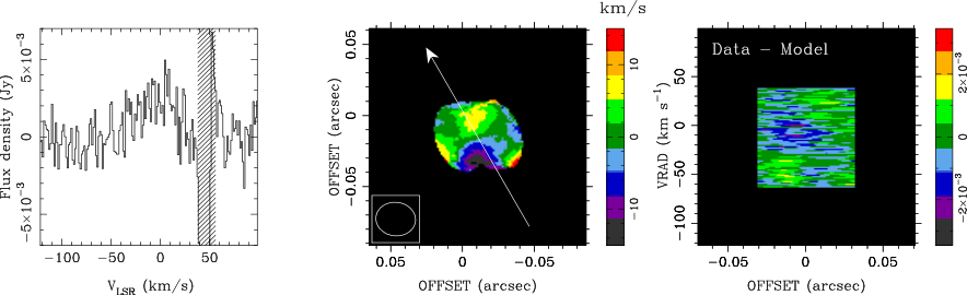
Another caveat of the expanding disk model is that while the moment 1 un-convolved model (middle-bottom panel in Figure 5) does indeed produce the expected curvature of the locus of gas at the (the green hue velocities), after convolution the effect is subtle (middle-middle panel). A more distinct effect produced by the presence of the expanding radial wind is the inclination of the velocity gradient respect to the longest projected axis of the disk. This effect is also subtle, but more noticeable even after convolution. In fact, a disk without expansion but inclined with P.A. gives only a slightly worse fit compared with that of Table 4. Appendix A shows the best-fit model results in this case. Convolving the model with the clean beam is a simple approximation of the observational distortions introduced by the interferometer. A more rigorous approach would be to perform simulated observations of the model matching the observational parameters. In Appendix B we show moment 1 maps of simulated observations of the model described above, the main finding being that the S -shape feature is slightly better preserved compared with the simple convolution. While advantageous in this regard, the computational costs of implementing simulations to optimize the parameters put such approach outside the scope of this paper.
The residuals, caveats, and overall comparison between the model and the data indicate that the disk model is certainly an oversimplification. However, we think it captures important features of the H38 and free-free continuum emission from G345.49+1.47. Considering that our current data is able to resolve the velocity gradient with about three beams across, we refrain in this work, from including additional sophistication to the model. The main difficulty we have now is the disagreement between the rotating compact system and the more extended emission.
IV.3 Expansion of the HC Hii Region and Photo-Ionized Wind.
One of the most obvious characteristics of the data, which is not well explained by a rotating disk, is the elongation of the source in the jet direction. This feature is also shown in Guzmán et al. 2014: their Source 10 (corresponding to G345.49+1.47) seems elongated in the east-west direction, which corresponds roughly to the jet direction. This elongation is not readily observed in the 02 resolution data of Cesaroni et al. 2017.
The elongation of the source can be explained by the expansion and consequently increase in size of the HC Hii region expected to occur in the directions where the material is less dense, that is, towards the symmetry axis. The lower density is associated with a larger distance that ionizing photons can travel before being absorbed. Density and opacity variations in the expanding gas explain the spectral index of the source and its variation in size with frequency (Guzmán et al. 2016).
The dynamics of the HC Hii region, whatever its geometry, depends crucially on how its size compares with the Bondi-Parker or sonic radius
| (4) |
where is the sound speed of the ionized gas (Sartorio et al. 2019; Keto 2007; Hollenbach et al. 1994). Roughly speaking, hydrostatic solutions can be maintained by the gravity of the central star against the pressure gradient of the ionized gas if the size of the Hii region is less than (or , Hollenbach et al. 1994). If the ionized region extends beyond this size, then it can begin its classical pressure-driven expansion (Dyson & Williams 1997, e.g.,) which has been successfully used to describe the evolution of compact Hii regions (Garay & Lizano 1999).
In the case of G345.49+1.47 and the best-fit parameters in Table 4, 178 au. We highlight that even in the lower limit of the stellar mass (15 suggested by Guzmán et al. 2014) we obtain au. Therefore, as shown in Figure 1, the ionized region we are probing likely lies inside the Bondi radius. Because this size is too small to explain the cm- and 3 mm-wavelength data (Guzmán et al. 2016; Guzmán et al. 2014), there are two possible explanations: (i) the region extends in the polar directions up to the Bondi radius (and beyond) but the low brightness and large scale filtering precludes the detection of this emission, and (ii) the region we are observing is confined, but it does not absorb all of the ionizing radiation from the HMYSO. The remaining uv-radiation escapes through the polar regions to ionize farther than , extending the size of the ionized region. Observations covering intermediate wavelengths between 1.3 and 3 mm may help to determine what is the true geometry of the HC Hii region.
In the previous section, we argue that including a radial expansion component may help explain some characteristics of the H38 moment 1 map. The best-fit parameters of this wind indicate it is transonic, with Mach number . The nature of this wind, however, is not clear. A first option is that it corresponds to a pressure driven wind (Parker 1958), which would remain subsonic inside . However, at distances comparable with the size of the disk au, the velocity derived for this wind is too small compared with the best-fit solution. Indeed, the Mach number at a distance from the origin is given by (Lamers & Cassinelli 1999)
| (5) |
which is lower by a factor of at least compared with the derived . We therefore rule out this wind coming from pressure driven expansion.
A second alternative is that this wind corresponds to photoionized gas being dragged by a stellar wind. These winds are common around high-mass stars but they are usually too tenuous to dominate the free-free and HRL emission. A stellar wind in G345.49+1.47 likewise helps to explain the relatively small best-fit disk width. Indeed, a strong stellar wind is expected to reduce the scale height of the photoionized disk, specially near a high-mass star (Hollenbach et al. 1994). However, the velocities of dragged photoionized winds are also predicted to be somewhat higher than the ones fitted to G345.49+1.47 (Yorke & Welz 1996). A third alternative is that this wind is somewhat linked to the accretion process, specifically, that the wind corresponds to magneto-centrifugal acceleration. This disk wind then would help the disk to lose angular momentum, facilitating the transport of material to smaller radii and eventually accrete into the HMYSO. This alternative has some support on the fact that G345.49+1.47 is associated with a fast, active jet and with evidence of accretion in the last hundreds of years. However, the acceleration expected (Tsinganos 2007, Equation (51)) from such a mechanism also produces much larger velocities than the ones observed shortly ( yr) after ejection. At this point and with the current data, the true nature of the G345.49+1.47 wind remains speculative.
IV.4 An Oppositely Rotating Molecular Envelope
The first indication of rotation derived from angular momentum conservation and contraction in G345.49+1.47 was provided by Guzmán et al. 2014, who found that sulfur oxide molecule transitions traced a rotating molecular core of size au around the HMYSO. The rotation axis was found to align well with the jet axis. No other molecular specie exhibit this kinematic feature (Guzmán et al. 2018) and a search for a more compact rotating structure in CH3CN proved inconclusive at best (Cesaroni et al. 2017).
Figure 7 shows the moment 1 of the SO2 transition ( K) adjacent to the H38 line (see Section III) compared with the 3 mm SO2 ( K) moment 1 presented in Guzmán et al. 2014. The SO2 moment 1 image was calculated using the CASA task immoments between and km s-1 and considering only emission above the 2 level. While our data is heavily filtered out due to the lack of short baseline coverage, the moment 1 shows a velocity pattern roughly consistent with that traced by SO2 at 3 mm, although more aligned in the E-W direction and tracing a higher velocity gradient. In fact, the SO2 velocity pattern closer to the HMYSO presented in this work seems more aligned with the jet and outflow.

The most noticeable feature of the rotating pattern of SO and SO2 at large scales is that it seems to run opposite to the rotation pattern of H38. The radius of the SO2 rotating core reported by Guzmán et al. 2014 is au, while the mm HRLs probe sizes 40 times smaller. Considering the difference in physical scales probed, it is not clear that the spin orientation of the smaller scale structure should necessarily inherit that of the larger structure. For example, Bate 2018 finds in simulations significant misalignment between the inner and outer parts of circumstellar disks, even in sources formed in relative isolation.
Remarkably, this feature has already been observed also toward relatively “evolved” HMYSOs — such as G345.49+1.47 — in at least two other cases: in Orion Src I, Zapata et al. 2012 reported an elongated, au across structure in SiO rotating in the opposite direction compared to the inner disk (Hirota et al. 2017); and in G17.64+0.16, Maud et al. 2018 found (also in SiO) that the lower velocity, extended structure of au across rotates in the opposite direction compared to the inner, au disk (Maud et al. 2019).
Barring chance coincidence and combination of motions associated , there are few theoretical physical explanations for these observed anti-alignments. First, in a crowded environment like a high-mass star forming region, it is possible that a combination of rotation and outflow motions associated with different sources could resemble an oppositely rotating envelope (Takakuwa et al. 2015). Second, an oppositely rotating, expanding outer envelope is predicted by the effect of Hall currents in magnetized disks (Tsukamoto et al. 2015). These currents are expected to be important when the Hall scale becomes comparable with the size of the system (Mininni et al. 2003). For G345.49+1.47 assuming a completely ionized hydrogen plasma system of density cm-3 and velocities comparables with the Keplerian speed at a scale of 100 au (few tens of km s-1), the Hall scale is extremely small (less than 1 m) even for a magnetic field as large as a milli-Gauss. It is possible, however, that the Hall current effect becomes more noticeable farther from the HMYSO, where the ionization fraction becomes much lower. Finally, we note that there are similitudes between the chemistry in the three sources mentioned above: rotation is not probed by the typical hydrogenated hot-core tracer molecules, but rather silicon and sulfur oxides, and water (the latter in Src I and G17.64+0.16 at least). Guzmán et al. 2018 suggest that the chemical signature of the rotating core in G345.49+1.47 resembles somewhat that of envelopes of evolved stars, being heavily influenced by the strong UV radiation. This view is also consistent with the results on the Orion Src I disk presented by Ginsburg et al. 2019.
IV.5 Accretion onto G345.49+1.47
One important characteristics of G345.49+1.47 is that it is associated with a fast protostellar jet (Guzmán et al. 2016). This jet has excited at least two pairs of roughly symmetrical ionized lobes whose proper motions indicate that one pair was probably ejected about yr ago and the other yr ago. The accretion rate associated is yr-1. Can the disk around G345.49+1.47 sustain these accretion rates?
First, the ionized mass in the disk is negligible, reaching only about , obtained by integrating the electron density (Equation (3)) times (the mean mass per electron in a fully ionized Hii and Hei region). However, it is possible that most of the disk mass is neutral near the midplane, and that the ionized component consists of two layers on the surface of the disk. We can constrain the circumstellar mass of G345.49+1.47 by using the continuum excess over the free-free derived in Section IV.1 (119 mJy) and the upper limit on the dust emission at 92 GHz of 11 mJy set by Guzmán et al. 2014. For that, we assume that the thermal dust emission comes from an homogeneous source covering a solid angle arcsec2 (Figure 2), whose flux density is given by
| (6) |
where is the dust temperature, its mass, and is the distance to the source. The dust opacity is given by with and cm2 gr-1 is the dust opacity (Ossenkopf & Henning 1994) including a gas-to-dust mass ratio of 100. Taking into account the flux limit at both frequencies and considering that should be less than the dust sublimation temperature (Kama et al. 2009, typically 1500 K, e.g.,) we obtain and , respectively.
A disk mass of 0.3–1.0 could sustain accretion rates of yr-1 (the lower bound of the accretion rate onto G345.49+1.47, Guzmán et al. 2016) for 30,000–100,000 yr, a time comparable with estimations of the jet phase duration (Purser et al. 2016; Guzmán et al. 2012, approximately yr). However, even if the entire disk were accreted, it would only affect minimally the mass of the HMYSO. Consistent with the disk not being too massive, we found no clear molecular counterpart of this disk in the rest of the frequency coverage of our data.
The estimation of the range of disk mass entails considering two scenarios for G345.49+1.47:
- (i)
Accretion onto the HMYSO has essentially ended. The observed disk is a remnant which could sustain some accretion, as evidenced by the jet activity, which cannot add a significant amount of mass to the HMYSO.
- (ii)
Accretion will resume in the future. We pose that accretion at this stage is very sporadic, with bursts of accretion which deplete a large fraction of the disk alternated between quiescent episodes with virtually no accretion, which would be the stage in which G345.49+1.47 is now. The environment of the HMYSO may replenish the disk and allow further accretion episodes in the future.
Because there are in the IRAS 165323959 molecular clump, which is in global contraction (Guzmán et al. 2011), scenario (ii) is still plausible. Accretion bursts associated with HMYSOs have already been observed (Caratti o Garatti et al. 2017; Hunter et al. 2017, e.g.,) and they can be substantial for the final mass of the star.
We propose the following picture for HMYSOs in a evolutionary stage similar to G345.49+1.47. Just after an accretion burst, the HMYSO cannot adjust immediately, causing it to expand and cool down (Hosokawa & Omukai 2009). The lack of ionizing radiation allows material at au to approach the HMYSO and replenish the disk more easily. However, if the timescale for disk replenishment becomes longer than the Kelvin-Helmholtz contraction timescale of the last accretion burst, the HMYSO will start to produce ionizing photons. This ionizing radiation is not effective in stopping accretion in the immediate vicinity of the young star, but it can disperse the material on larger ( au) scales (Kuiper & Hosokawa 2018), effectively halting further replenishment of the accretion disk. Therefore, that the cycle described in (ii) perdures or becomes scenario (i) depends on the environment much farther away than the size of the disk, and on how the ionizing radiation will affect this environment.
This very dynamic picture of accretion may help to explain some of the observed variability of HC Hii regions (Galván-Madrid et al. 2008; De Pree et al. 2014; De Pree et al. 2015). A sufficiently massive accretion burst may completely choke a young HC Hii region, and the HMYSO will start again a new cycle of expansion and contraction. Likewise, the picture may help to understand why HMYSOs with apparently little material in their close environment (suggesting more evolved sources) such as Orion Src I (Plambeck & Wright 2016) and IRAS 134816124 are not associated with Hii regions. In this view, the immediate environment was possibly cleared out in the last accretion burst, and the star is still contracting.
This idea may provide a picture which explains the oppositely rotating large scale cores described in Section IV.4. In principle, if the disk is mostly consumed after an accretion burst, new replenishing material should not necessarily form a disk with the same orientation or plane. However, we must consider that the environment of the HMYSO is not homogeneous, but it has already been shaped by the previous outflows. In this way, the history of accretion shaping the environment makes it likely that the new material will accrete through a similar plane as their predecessor. The argument does not preclude new material from having an opposite rotation.
IV.6 A likely binary system.
High-mass stars commonly form in binary systems (Chini et al. 2012, e.g.,). In the case of G345.49+1.47, until now there has been no evidence that it is a binary. However, the detection of Source 10a suggests that this young star may be a stellar companion of the HMYSO. Alternative hypotheses are that Source 10a is far away from G345.49+1.47, and only close in projection, or that it is a high-velocity fly-by young star.
Considering that Source 10a is at a projected separation of 690 au from G345.49+1.47, we correct this distance by assuming a random orientation between these sources, obtaining 880 au. To determine whether a binary system with this separation is plausible in the center of the IRAS 165623959 cluster environment, we compare the orbital energy of the purported binary with the average energy of stellar encounters (Binney & Tremaine 2008, Chapter 8). To evaluate the latter, we assume that the 3D velocity dispersion of the young stars is the same as the observed velocity dispersion of the gas. Measurements of of the gas toward IRAS 165623959 range between 4 and 7 km s-1 depending on the molecular tracer (Guzmán et al. 2018; Miettinen et al. 2006; Bronfman et al. 1996), so, we use km s-1(or km s-1) as an average value. The criterion which defines a so-called hard binary in this environment is
| (7) |
where is the binay separation, and are the masses of both stars, and the typical clump stellar mass. If the system does not fulfill (7), then it is prone to disruption by gravitational interaction with other cluster members. Since the distances involved are small compared with the clump size, we ignore the perturbing effect of the gas mass potential. Further assuming that the mass of Source 10a is comparable to the typical individual mass of the stellar component of IRAS 165323959, then Equation (7) simply means that the orbital velocity around G345.49+1.47 should be larger than the velocity dispersion of the clump.
Using au and , we obtain that the orbital velocity is 5.8 km s-1, larger than km s-1. We conclude that G345.49+1.47 and Source 10a likely form a binary system. The location from the HMYSO makes Source 10a having formed from disk fragmentation rather unlikely. Only recently ALMA has provided the opportunity to witness how binaries containing high-mass stars form. In two recent studies, Ilee et al. 2018 finds that a high-mass star has a companion that is likely a low-mass protostar (as in G345.49+1.47), while Zhang et al. 2019a find a binary system in which both stars are massive and are associated with HCHii regions.
V Conclusions.
We present high spatial resolution observations of G345.49+1.47, made using ALMA, targeting the H38 HRL and the 1.3 mm continuum emission. The main conclusions of this study can be summarized as follows:
- 1.
The H38 HRL reveals a au ionized disk around G345.49+1.47, rotating perpendicularly to the previously detected ionized jet.
- 2.
The sense of rotation observed in the ionized gas is opposite to that detected in sulfur oxides at larger scales.
- 3.
The disk has sustained accretion and jet ejection episodes during the past hundreds of years. We estimate the disk mass to be in the 0.3–1.0 range, suggesting it is not relevant for the final mass of G345.49+1.47. This disk may sustain an accretion rate of yr-1 (Guzmán et al. 2016) for 30,000–100,000 yr, comparable with estimates of the jet phase duration.
- 4.
We propose that the accretion onto G345.49+1.47, and sources alike, is sporadic with strong bursts of accretion which consume a large fraction of the disk. We speculate that G345.49+1.47 is actually between these accretion episodes.
- 5.
The H38 moment 1 map suggest the presence of a radial, expanding transonic wind in addition to rotation.
- 6.
We report in this work the detection of Source 10a, a likely low-mass YSO. This source is probably a binary stellar companion of G345.49+1.47.
Appendix A Disk Models with Different Parameters
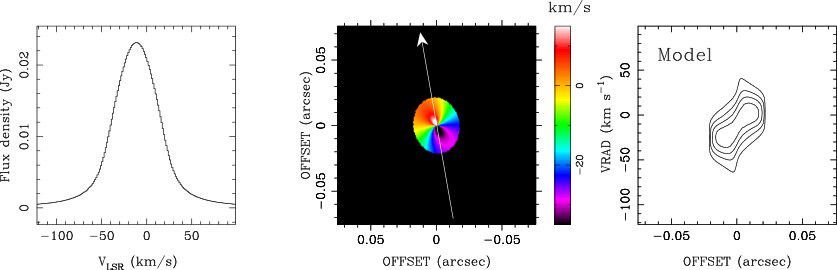
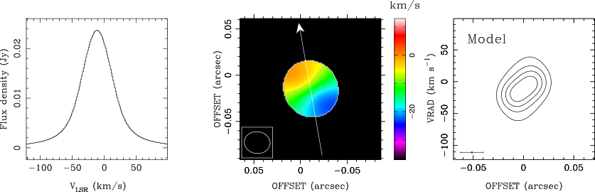
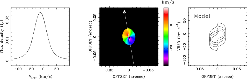
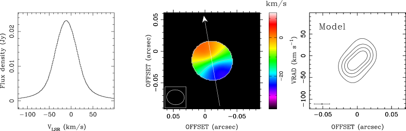
We show best-fit results for the disk model using different set of parameters. Models A.1 shows the best-fit results assuming that the disk width increases with radius as , with as in the prescription of Hollenbach et al. 1994. Models A.2 and A.3 show the best-fit models assuming a mass of 15 and 56 , which span conservatively the uncertainty due to the flashlight effect and the range of masses given in the literature for G345.49+1.47. Models A.4 to A.6 show the fitted model with the same masses as in models A1 to A3, but with P.A.°.
| Parameter | Best-fit values | |||||
|---|---|---|---|---|---|---|
| A.1 | A.2 | A.3 | A.4 | A.5 | A.6 | |
| km s-1 | km s-1 | km s-1 | km s-1 | km s-1 | km s-1 | |
| P.A. | (fixed) | (fixed) | (fixed) | (fixed) | (fixed) | (fixed) |
| ††footnotemark: | ||||||
| (fixed) | (fixed) | (fixed) | (fixed) | (fixed) | (fixed) | |
| K (fixed) | K (fixed) | K (fixed) | K (fixed) | K (fixed) | K (fixed) | |
| au | au | au | au | au | au | |
| km s-1 | km s-1 | km s-1 | km s-1 | km s-1 | km s-1 | |
| au | au | au | au | au | ||
Note. — Using our notation, the inclination of the disk axis respect to the plane of the sky is .






Appendix B Simulated observations
In order to compare the data with the model and determine the best fit parameters, the approach followed in this paper (Section 4) is simply to convolve the model with the clean beam to introduce the effect of limited resolution. Whereas this process is relatively simple and computationally cheap, the clean beam is only an approximation of one aspect of the instrumental effect and observational uncertainties introduced by the telescope. In order to reproduce better the instrumental response, we simulated observations of a theoretical brightness model (third row of Figure 5) using the CASA task simobserve. We created the configuration antenna file for the two execution blocks of our observations using the buildConfigurationFile task of the CASA extensions33 3 https://safe.nrao.edu/wiki/bin/view/ALMA/BuildConfigurationFile. After that, using the same LST range as with our visibilities, we run simobserve to create the simulated measurement sets.
We restored the cubes to the image plane and deconvolved the simulated datacubes using the task tclean with the same parameters as described in Section 2. Given the width of the HRL, this process requires generating cubes of around 200 channels wide at least. Because of the very long baselines involved in our observations, adequately sampling the beam response and avoiding aliasing entails creating large cubes of pixels per channel. Partly because of this computational cost, we decided not to implement this approach in the optimization steps.
Figure 16 shows the result of the simulated observations of the best-fit model whose parameters are in Table 4. Panels (a) to (d) show the the moment 1 of the simobserve cube including simulated observational noise into the uv-data, the observed moment 1 map, the moment 1 of the model, and the moment 1 of the simobserve cube deconvolved from simulated noiseless uv-data, respectively. Panels (a) and (d) show that the S signature in the moment 1 seems to be better preserved in this simulation compared to the clean beam convolution. However, we note that this depends somewhat on the noise level up to which we can effectively calculate the moment 1; the S -shape feature being more conspicuous the less bright emission in the moment 1 calculation is included.

References
- Andrae et al. (2018) Andrae, R., Fouesneau, M., Creevey, O., et al. 2018, A&A, 616, A8, doi: 10.1051/0004-6361/201732516
- Bally & Zinnecker (2005) Bally, J., & Zinnecker, H. 2005, AJ, 129, 2281, doi: 10.1086/429098
- Bate (2018) Bate, M. R. 2018, MNRAS, 475, 5618, doi: 10.1093/mnras/sty169
- Beltrán et al. (2016) Beltrán, M. T., Cesaroni, R., Moscadelli, L., et al. 2016, A&A, 593, A49, doi: 10.1051/0004-6361/201628588
- Beltrán & de Wit (2016) Beltrán, M. T., & de Wit, W. J. 2016, A&A Rev., 24, 6, doi: 10.1007/s00159-015-0089-z
- Beuther et al. (2017) Beuther, H., Linz, H., Henning, T., Feng, S., & Teague, R. 2017, A&A, 605, A61, doi: 10.1051/0004-6361/201730575
- Binney & Tremaine (2008) Binney, J., & Tremaine, S. 2008, Galactic Dynamics: Second Edition
- Boley et al. (2016) Boley, P. A., Kraus, S., de Wit, W.-J., et al. 2016, A&A, 586, A78, doi: 10.1051/0004-6361/201527502
- Briggs (1995) Briggs, D. S. 1995, PhD thesis, New Mexico Institute of Mining and Technology, USA. http://www.aoc.nrao.edu/dissertations/dbriggs/
- Bronfman et al. (1996) Bronfman, L., Nyman, L. A., & May, J. 1996, A&AS, 115, 81
- Caratti o Garatti et al. (2016) Caratti o Garatti, A., Stecklum, B., Weigelt, G., et al. 2016, A&A, 589, L4, doi: 10.1051/0004-6361/201628203
- Caratti o Garatti et al. (2017) Caratti o Garatti, A., Stecklum, B., Garcia Lopez, R., et al. 2017, Nature Physics, 13, 276, doi: 10.1038/nphys3942
- Carrasco-González et al. (2015) Carrasco-González, C., Torrelles, J. M., Cantó, J., et al. 2015, Science, 348, 114, doi: 10.1126/science.aaa7216
- Cesaroni et al. (2006) Cesaroni, R., Galli, D., Lodato, G., Walmsley, M., & Zhang, Q. 2006, Nature, 444, 703, doi: 10.1038/nature05344
- Cesaroni et al. (2017) Cesaroni, R., Sánchez-Monge, Á., Beltrán, M. T., et al. 2017, A&A, 602, A59, doi: 10.1051/0004-6361/201630184
- Cesaroni et al. (2018) Cesaroni, R., Moscadelli, L., Neri, R., et al. 2018, A&A, 612, A103, doi: 10.1051/0004-6361/201732238
- Chen et al. (2016) Chen, H.-R. V., Keto, E., Zhang, Q., et al. 2016, ApJ, 823, 125, doi: 10.3847/0004-637X/823/2/125
- Chini et al. (2012) Chini, R., Hoffmeister, V. H., Nasseri, A., Stahl, O., & Zinnecker, H. 2012, MNRAS, 424, 1925, doi: 10.1111/j.1365-2966.2012.21317.x
- Cooper et al. (2013) Cooper, H. D. B., Lumsden, S. L., Oudmaijer, R. D., et al. 2013, MNRAS, 430, 1125, doi: 10.1093/mnras/sts681
- Curiel et al. (2006) Curiel, S., Ho, P. T. P., Patel, N. A., et al. 2006, ApJ, 638, 878, doi: 10.1086/498931
- Davies et al. (2011) Davies, B., Hoare, M. G., Lumsden, S. L., et al. 2011, MNRAS, 416, 972, doi: 10.1111/j.1365-2966.2011.19095.x
- Davies et al. (2010) Davies, B., Lumsden, S. L., Hoare, M. G., Oudmaijer, R. D., & de Wit, W.-J. 2010, MNRAS, 402, 1504, doi: 10.1111/j.1365-2966.2009.16077.x
- De Pree et al. (2014) De Pree, C. G., Peters, T., Mac Low, M. M., et al. 2014, ApJ, 781, L36, doi: 10.1088/2041-8205/781/2/L36
- De Pree et al. (2015) —. 2015, ApJ, 815, 123, doi: 10.1088/0004-637X/815/2/123
- Dyson & Williams (1997) Dyson, J. E., & Williams, D. A. 1997, The physics of the interstellar medium, doi: 10.1201/9780585368115
- Gaia Collaboration et al. (2016) Gaia Collaboration, Prusti, T., de Bruijne, J. H. J., et al. 2016, A&A, 595, A1, doi: 10.1051/0004-6361/201629272
- Gaia Collaboration et al. (2018) Gaia Collaboration, Brown, A. G. A., Vallenari, A., et al. 2018, A&A, 616, A1, doi: 10.1051/0004-6361/201833051
- Galván-Madrid et al. (2008) Galván-Madrid, R., Rodríguez, L. F., Ho, P. T. P., & Keto, E. 2008, ApJ, 674, L33, doi: 10.1086/528957
- Garay & Lizano (1999) Garay, G., & Lizano, S. 1999, PASP, 111, 1049, doi: 10.1086/316416
- Ginsburg et al. (2018) Ginsburg, A., Bally, J., Goddi, C., Plambeck, R., & Wright, M. 2018, ApJ, 860, 119, doi: 10.3847/1538-4357/aac205
- Ginsburg et al. (2019) Ginsburg, A., McGuire, B., Plambeck, R., et al. 2019, ApJ, 872, 54, doi: 10.3847/1538-4357/aafb71
- Girart et al. (2017) Girart, J. M., Estalella, R., Fernández-López, M., et al. 2017, ApJ, 847, 58, doi: 10.3847/1538-4357/aa81c9
- Goddi et al. (2018) Goddi, C., Ginsburg, A., Maud, L., Zhang, Q., & Zapata, L. 2018, arXiv e-prints, arXiv:1805.05364. https://arxiv.org/abs/1805.05364
- Gordon & Sorochenko (2002) Gordon, M. A., & Sorochenko, R. L. 2002, Radio Recombination Lines. Their Physics and Astronomical Applications, Vol. 282, doi: 10.1007/978-0-387-09604-9
- Guzmán et al. (2010) Guzmán, A. E., Garay, G., & Brooks, K. J. 2010, ApJ, 725, 734, doi: 10.1088/0004-637X/725/1/734
- Guzmán et al. (2011) Guzmán, A. E., Garay, G., Brooks, K. J., Rathborne, J., & Güsten, R. 2011, ApJ, 736, 150, doi: 10.1088/0004-637X/736/2/150
- Guzmán et al. (2012) Guzmán, A. E., Garay, G., Brooks, K. J., & Voronkov, M. A. 2012, ApJ, 753, 51, doi: 10.1088/0004-637X/753/1/51
- Guzmán et al. (2016) Guzmán, A. E., Garay, G., Rodríguez, L. F., et al. 2016, ApJ, 826, 208, doi: 10.3847/0004-637X/826/2/208
- Guzmán et al. (2018) Guzmán, A. E., Guzmán, V. V., Garay, G., Bronfman, L., & Hechenleitner, F. 2018, ApJS, 236, 45, doi: 10.3847/1538-4365/aac01d
- Guzmán et al. (2014) Guzmán, A. E., Garay, G., Rodríguez, L. F., et al. 2014, ApJ, 796, 117
- Guzmán (2020) Guzmán, A. E. 2020, Replication Data for "A photoionized accretion disk around a young high-mass star", Harvard Dataverse, doi: 10.7910/DVN/1OBDQQ
- Hennebelle et al. (2011) Hennebelle, P., Commerçon, B., Joos, M., et al. 2011, A&A, 528, A72, doi: 10.1051/0004-6361/201016052
- Hirota et al. (2017) Hirota, T., Machida, M. N., Matsushita, Y., et al. 2017, Nature Astronomy, 1, 0146, doi: 10.1038/s41550-017-0146
- Hollenbach et al. (1994) Hollenbach, D., Johnstone, D., Lizano, S., & Shu, F. 1994, ApJ, 428, 654, doi: 10.1086/174276
- Hosokawa & Omukai (2009) Hosokawa, T., & Omukai, K. 2009, ApJ, 691, 823, doi: 10.1088/0004-637X/691/1/823
- Hosokawa et al. (2010) Hosokawa, T., Yorke, H. W., & Omukai, K. 2010, ApJ, 721, 478, doi: 10.1088/0004-637X/721/1/478
- Hunter et al. (2017) Hunter, T. R., Brogan, C. L., MacLeod, G., et al. 2017, ApJ, 837, L29, doi: 10.3847/2041-8213/aa5d0e
- Ilee et al. (2018) Ilee, J. D., Cyganowski, C. J., Brogan, C. L., et al. 2018, ApJ, 869, L24, doi: 10.3847/2041-8213/aaeffc
- Ilee et al. (2016) Ilee, J. D., Cyganowski, C. J., Nazari, P., et al. 2016, MNRAS, 462, 4386, doi: 10.1093/mnras/stw1912
- James & Roos (1975) James, F., & Roos, M. 1975, Computer Physics Communications, 10, 343, doi: 10.1016/0010-4655(75)90039-9
- Jiménez-Serra et al. (2011) Jiménez-Serra, I., Martín-Pintado, J., Báez-Rubio, A., Patel, N., & Thum, C. 2011, ApJ, 732, L27, doi: 10.1088/2041-8205/732/2/L27
- Johnston et al. (2015) Johnston, K. G., Robitaille, T. P., Beuther, H., et al. 2015, ApJ, 813, L19, doi: 10.1088/2041-8205/813/1/L19
- Kahn (1974) Kahn, F. D. 1974, A&A, 37, 149
- Kama et al. (2009) Kama, M., Min, M., & Dominik, C. 2009, A&A, 506, 1199, doi: 10.1051/0004-6361/200912068
- Keto (2007) Keto, E. 2007, ApJ, 666, 976, doi: 10.1086/520320
- Kuiper & Hosokawa (2018) Kuiper, R., & Hosokawa, T. 2018, A&A, 616, A101, doi: 10.1051/0004-6361/201832638
- Kuiper et al. (2010) Kuiper, R., Klahr, H., Beuther, H., & Henning, T. 2010, ApJ, 722, 1556, doi: 10.1088/0004-637X/722/2/1556
- Lamers & Cassinelli (1999) Lamers, H. J. G. L. M., & Cassinelli, J. P. 1999, Introduction to Stellar Winds (Cambridge University Press). http://dx.doi.org/10.1017/CBO9781139175012
- Larson & Starrfield (1971) Larson, R. B., & Starrfield, S. 1971, A&A, 13, 190
- Lumsden et al. (2013) Lumsden, S. L., Hoare, M. G., Urquhart, J. S., et al. 2013, ApJS, 208, 11, doi: 10.1088/0067-0049/208/1/11
- Luri et al. (2018) Luri, X., Brown, A. G. A., Sarro, L. M., et al. 2018, A&A, 616, A9, doi: 10.1051/0004-6361/201832964
- Masqué et al. (2015) Masqué, J. M., Rodríguez, L. F., Araudo, A., et al. 2015, ApJ, 814, 44, doi: 10.1088/0004-637X/814/1/44
- Maud et al. (2018) Maud, L. T., Cesaroni, R., Kumar, M. S. N., et al. 2018, A&A, 620, A31, doi: 10.1051/0004-6361/201833908
- Maud et al. (2019) —. 2019, A&A, 627, L6, doi: 10.1051/0004-6361/201935633
- McMullin et al. (2007) McMullin, J. P., Waters, B., Schiebel, D., Young, W., & Golap, K. 2007, in Astronomical Society of the Pacific Conference Series, Vol. 376, Astronomical Data Analysis Software and Systems XVI, ed. R. A. Shaw, F. Hill, & D. J. Bell, 127
- Miettinen et al. (2006) Miettinen, O., Harju, J., Haikala, L. K., & Pomrén, C. 2006, A&A, 460, 721, doi: 10.1051/0004-6361:20064815
- Mininni et al. (2003) Mininni, P. D., Gómez, D. O., & Mahajan, S. M. 2003, ApJ, 584, 1120, doi: 10.1086/345777
- Mocanu et al. (2013) Mocanu, L. M., Crawford, T. M., Vieira, J. D., et al. 2013, ApJ, 779, 61, doi: 10.1088/0004-637X/779/1/61
- Moisés et al. (2011) Moisés, A. P., Damineli, A., Figuerêdo, E., et al. 2011, MNRAS, 411, 705, doi: 10.1111/j.1365-2966.2010.17713.x
- Moscadelli et al. (2013) Moscadelli, L., Cesaroni, R., Sánchez-Monge, Á., et al. 2013, A&A, 558, A145, doi: 10.1051/0004-6361/201321951
- Moscadelli et al. (2019) Moscadelli, L., Sanna, A., Cesaroni, R., et al. 2019, A&A, 622, A206, doi: 10.1051/0004-6361/201834366
- Motogi et al. (2019) Motogi, K., Hirota, T., Machida, M. N., et al. 2019, ApJ, 877, L25, doi: 10.3847/2041-8213/ab212f
- Motogi et al. (2013) Motogi, K., Sorai, K., Niinuma, K., et al. 2013, MNRAS, 428, 349, doi: 10.1093/mnras/sts035
- Mottram et al. (2011) Mottram, J. C., Hoare, M. G., Urquhart, J. S., et al. 2011, A&A, 525, A149, doi: 10.1051/0004-6361/201014479
- Nakano (1989) Nakano, T. 1989, ApJ, 345, 464, doi: 10.1086/167919
- Obonyo et al. (2019) Obonyo, W. O., Lumsden, S. L., Hoare, M. G., et al. 2019, MNRAS, 486, 3664, doi: 10.1093/mnras/stz1091
- Orozco-Aguilera et al. (2017) Orozco-Aguilera, M. T., Zapata, L. A., Hirota, T., Qin, S.-L., & Masqué, J. M. 2017, ApJ, 847, 66, doi: 10.3847/1538-4357/aa88cd
- Ossenkopf & Henning (1994) Ossenkopf, V., & Henning, T. 1994, A&A, 291, 943
- Paladini et al. (2004) Paladini, R., Davies, R. D., & De Zotti, G. 2004, MNRAS, 347, 237, doi: 10.1111/j.1365-2966.2004.07210.x
- Parker (1958) Parker, E. N. 1958, ApJ, 128, 664, doi: 10.1086/146579
- Peters et al. (2012) Peters, T., Klaassen, P. D., Mac Low, M.-M., Klessen, R. S., & Banerjee, R. 2012, ApJ, 760, 91, doi: 10.1088/0004-637X/760/1/91
- Pickett et al. (1998) Pickett, H. M., Poynter, R. L., Cohen, E. A., et al. 1998, J. Quant. Spec. Radiat. Transf., 60, 883, doi: 10.1016/S0022-4073(98)00091-0
- Plambeck & Wright (2016) Plambeck, R. L., & Wright, M. C. H. 2016, ApJ, 833, 219, doi: 10.3847/1538-4357/833/2/219
- Pomohaci et al. (2017) Pomohaci, R., Oudmaijer, R. D., Lumsden, S. L., Hoare, M. G., & Mendigutía, I. 2017, MNRAS, 472, 3624, doi: 10.1093/mnras/stx2196
- Purser et al. (2016) Purser, S. J. D., Lumsden, S. L., Hoare, M. G., et al. 2016, MNRAS, 460, 1039, doi: 10.1093/mnras/stw1027
- Remijan et al. (2019) Remijan, A., Biggs, A., Cortes, P., et al. 2019. https://almascience.nrao.edu/documents-and-tools/cycle7/alma-technical-handbook/view
- Richer & Padman (1991) Richer, J. S., & Padman, R. 1991, MNRAS, 251, 707, doi: 10.1093/mnras/251.4.707
- Rodríguez et al. (2008) Rodríguez, L. F., Moran, J. M., Franco-Hernández, R., et al. 2008, AJ, 135, 2370, doi: 10.1088/0004-6256/135/6/2370
- Rodríguez-Kamenetzky et al. (2020) Rodríguez-Kamenetzky, A., Carrasco-González, C., Torrelles, J. M., et al. 2020, MNRAS, 496, 3128, doi: 10.1093/mnras/staa1742
- Rosero et al. (2019) Rosero, V., Hofner, P., Kurtz, S., et al. 2019, ApJ, 880, 99, doi: 10.3847/1538-4357/ab2595
- Sánchez-Monge et al. (2013) Sánchez-Monge, Á., Cesaroni, R., Beltrán, M. T., et al. 2013, A&A, 552, L10, doi: 10.1051/0004-6361/201321134
- Sanna et al. (2018) Sanna, A., Moscadelli, L., Goddi, C., Krishnan, V., & Massi, F. 2018, A&A, 619, A107, doi: 10.1051/0004-6361/201833573
- Sartorio et al. (2019) Sartorio, N. S., Vandenbroucke, B., Falceta-Goncalves, D., Wood, K., & Keto, E. 2019, MNRAS, 486, 5171, doi: 10.1093/mnras/stz1187
- Strelnitski et al. (1996) Strelnitski, V. S., Ponomarev, V. O., & Smith, H. A. 1996, ApJ, 470, 1118, doi: 10.1086/177936
- Takakuwa et al. (2015) Takakuwa, S., Kiyokane, K., Saigo, K., & Saito, M. 2015, ApJ, 814, 160, doi: 10.1088/0004-637X/814/2/160
- Tan et al. (2014) Tan, J. C., Beltrán, M. T., Caselli, P., et al. 2014, in Protostars and Planets VI, ed. H. Beuther, R. S. Klessen, C. P. Dullemond, & T. Henning, 149, doi: 10.2458/azu_uapress_9780816531240-ch007
- Titmarsh et al. (2013) Titmarsh, A. M., Ellingsen, S. P., Breen, S. L., Caswell, J. L., & Voronkov, M. A. 2013, ApJ, 775, L12, doi: 10.1088/2041-8205/775/1/L12
- Torrelles et al. (2007) Torrelles, J. M., Patel, N. A., Curiel, S., et al. 2007, ApJ, 666, L37, doi: 10.1086/521675
- Tsinganos (2007) Tsinganos, K. 2007, Theory of MHD Jets and Outflows, ed. J. Ferreira, C. Dougados, & E. Whelan, Vol. 723, 117
- Tsukamoto et al. (2015) Tsukamoto, Y., Iwasaki, K., Okuzumi, S., Machida, M. N., & Inutsuka, S. 2015, ApJ, 810, L26, doi: 10.1088/2041-8205/810/2/L26
- Wilson et al. (2013) Wilson, T., Rohlfs, K., & Huettemeister, S. 2013, Tools of Radio Astronomy, Astronomy and Astrophysics Library (Springer Berlin Heidelberg), doi: 10.1007/978-3-642-39950-3
- Wolfire & Cassinelli (1987) Wolfire, M. G., & Cassinelli, J. P. 1987, ApJ, 319, 850, doi: 10.1086/165503
- Yorke & Sonnhalter (2002) Yorke, H. W., & Sonnhalter, C. 2002, ApJ, 569, 846, doi: 10.1086/339264
- Yorke & Welz (1996) Yorke, H. W., & Welz, A. 1996, A&A, 315, 555
- Zapata et al. (2019) Zapata, L. A., Garay, G., Palau, A., et al. 2019, ApJ, 872, 176, doi: 10.3847/1538-4357/aafedf
- Zapata et al. (2015) Zapata, L. A., Palau, A., Galván-Madrid, R., et al. 2015, MNRAS, 447, 1826, doi: 10.1093/mnras/stu2527
- Zapata et al. (2012) Zapata, L. A., Rodríguez, L. F., Schmid-Burgk, J., et al. 2012, ApJ, 754, L17, doi: 10.1088/2041-8205/754/1/L17
- Zhang & Tan (2018) Zhang, Y., & Tan, J. C. 2018, ApJ, 853, 18, doi: 10.3847/1538-4357/aaa24a
- Zhang et al. (2014) Zhang, Y., Tan, J. C., & Hosokawa, T. 2014, ApJ, 788, 166, doi: 10.1088/0004-637X/788/2/166
- Zhang et al. (2019a) Zhang, Y., Tan, J. C., Tanaka, K. E. I., et al. 2019a, Nature Astronomy, 3, 517, doi: 10.1038/s41550-019-0718-y
- Zhang et al. (2019b) Zhang, Y., Tanaka, K. E. I., Rosero, V., et al. 2019b, ApJ, 886, L4, doi: 10.3847/2041-8213/ab5309
- Zinchenko et al. (2015) Zinchenko, I., Liu, S. Y., Su, Y. N., et al. 2015, ApJ, 810, 10, doi: 10.1088/0004-637X/810/1/10