Heteroscedastic Bayesian Optimisation for Stochastic Model Predictive Control

We consider a dynamical system with states $s\in{\mathcal{{S}}}$ and admissible controls (or actions) $a\in\mathcal{A}$ where the state follows Markovian dynamics, $s_{t+1}=f\left(s_{t},a_{t}\right)$, with a transition function $f$ and a reward function $r$ that measures how well the system is doing given a state and action $r:\mathcal{S}\times\mathcal{A}\to\mathbb{{R}}$. Although the true dynamics are usually unknown, a model of the transition function can be learned or assumed from expert knowledge.

Model predictive control, also known as receding horizon control, is a class of algorithms that operate by optimising sequences of actions over approximate models of a system. MPC solves an optimisation problem up to a horizon $T$ constrained by a dynamical system $f$ and then executes the next best action. The diagram in Fig. 2 describes the interaction between the system and the controller in MPC.

A flexible MPC method that optimises controls as an information-theoretic sampling-based algorithm is model predictive path integral (MPPI) [17]. At time step $t$, MPPI outputs sequences of noise-perturbed controls $\mathrm{{V}}_{t}=\{v_{i}\}_{i=t}^{t+T}$, where $v_{i}=a_{i}^{*}+\epsilon_{i}$ and $\epsilon_{i}\sim\mathcal{N}(0,\sigma_{\epsilon}^{2})$, based on a rollover sequence of optimal actions $\{a_{i}^{*}\}_{i=t}^{t+T}$ that start as 0.

When applied to a model of the system, each control sequence results in a sequence of states $\mathrm{{S}}_{t}=\{s_{t+i}\}_{i=1}^{T}$ with cost determined by a function associated with the control task:

where $c:{\mathcal{{S}}}\to\mathbb{{R}}^{+}$ is an instant cost function, and $\phi:{\mathcal{{S}}}\to\mathbb{{R}}^{+}$ represents terminal cost. Based on $M$ rollouts, MPPI updates the sequence of optimal actions and weights [3]:

and $\eta$ is a normalisation constant, so that $\sum_{j=1}^{M}w(\mathrm{{V}}_{t}^{j})=1$. MPPI then applies the first action in the sequence to the real system, discards it and appends a new random action to the end of the sequence. This process repeats every time step.

The second hyper-parameter appears in (3) and is called temperature $\lambda\in\mathbb{{R}}^{+}$. Intuitively, a higher variance $\sigma_{\epsilon}^{2}$ results in more varying and forceful actions, while $\lambda\to 0$ leads the optimal distribution to place all its mass on a single trajectory. Conversely, $\lambda\to\infty$ would make all trajectories have similar probabilities of occurrence [25].

Both hyper-parameters control exploration and exploitation. Higher $\lambda$ or $\sigma_{\epsilon}$ result in more exploration in the action space, while lower $\lambda$ or $\sigma_{\epsilon}$ result in more exploitation. That raises the question of how to find the best hyper-parameter settings, which may have to be tuned according to the task.

A Gaussian process [20] represents a probability distribution over a space of functions. A GP prior over a function $g:{\mathcal{{X}}}\to\mathbb{{R}}$ is completely specified by a mean $m:{\mathcal{{X}}}\to\mathbb{{R}}$ and a positive-definite covariance function, $k:{\mathcal{{X}}}\times{\mathcal{{X}}}\to\mathbb{{R}}$. Under the GP prior, the values of $g$ at a finite collection of points $\{{\boldsymbol{\mathbf{x}}}_{i}\}_{i=1}^{n}\subset{\mathcal{{X}}}$ follow a multivariate normal distribution $g({\boldsymbol{\mathbf{{{\boldsymbol{\mathbf{X}}}}}}})\sim\mathcal{N}({\boldsymbol{\mathbf{m}}},{\boldsymbol{\mathbf{{K}}}})$, where $g({\boldsymbol{\mathbf{{{\boldsymbol{\mathbf{X}}}}}}})=[g({\boldsymbol{\mathbf{x}}}_{1}),\dots,g({\boldsymbol{\mathbf{x}}}_{n})]^{\mathsf{T}}$, ${\boldsymbol{\mathbf{m}}}:=m({\boldsymbol{\mathbf{{{\boldsymbol{\mathbf{X}}}}}}})$, and ${\boldsymbol{\mathbf{{K}}}}$ is the $n$-by-$n$ covariance matrix given by $[{\boldsymbol{\mathbf{{K}}}}]_{i,j}=k({\boldsymbol{\mathbf{x}}}_{i},{\boldsymbol{\mathbf{x}}}_{j})$.

Consider the problem of searching for the global optimum of a function $g:{\mathcal{{X}}}\to\mathbb{R}$ over a given compact search space ${\mathcal{{S}}}\subset{\mathcal{{X}}}$ such as determining ${\boldsymbol{\mathbf{x}}}^{*}\in\operatornamewithlimits{argmax}_{{\boldsymbol{\mathbf{x}}}\in{\mathcal{{S}}}}g({\boldsymbol{\mathbf{x}}})$. Assume that $g$ is possibly non-convex and only partially observable via noisy estimates $y_{t}=g({\boldsymbol{\mathbf{x}}}_{t})+\nu_{t}$ with $\nu_{t}\sim\mathcal{N}(0,\sigma_{\nu_{t}}^{2})$. In addition, we can only observe the function up to $N$ times.

Bayesian optimisation [6] assumes that $g$ is a random variable itself and models it as a stochastic process, which is usually a GP, indexed by ${\mathcal{{X}}}$. To select points at which to observe $g$, BO uses an acquisition function $h({\boldsymbol{\mathbf{x}}})$ as a guide that incorporates prior information provided by the GP model and the observations. Each query point ${\boldsymbol{\mathbf{x}}}_{t}\in{\mathcal{{S}}}$ is then selected by maximising $h$. After collecting an observation $y_{t}$, BO updates the GP model with the pair $({\boldsymbol{\mathbf{x}}}_{t},y_{t})$ and starts the next iteration with an improved belief about $f$. The BO loop repeats until we reach the given budget of $N$ evaluations of the objective function. See Algorithm 1 for a summary.

The acquisition function $h$ determines which values to sample next. A common and simple acquisition function is the upper confidence bound (UCB) [26]:

where $\kappa\in\mathbb{{R}}^{+}$ is a balance factor. UCB allows balancing exploration and exploitation by valuing points where there is high uncertainty (exploration) or where the GP predictive mean is high (exploitation). Keeping the balance factor $\kappa$ biased towards exploration avoids local minima.

As a performance indicator, our framework consists of accumulating instant rewards over episodes, as shown in Fig. 3. An episode is defined as a sequence of controller-system interactions $\{s_{i},a_{i},s_{i+1},a_{i+1},\ldots\}$, and each action $a_{i}$ returns a respective reward $r_{i}$ from the system. We deal with fixed-length episodes, with a control loop executed up to time $n_{e}$. At each time step, the MPC’s optimal action is sent to the system actuators, obtaining a reward $r_{i}$ that is accumulated along the episode as $g=\sum_{i}^{n_{e}}r_{i}$. However, due to a number of factors, such as an arbitrary initial state, rewards are stochastic.

Our objective is to maximise the expected cumulative reward $\hat{g}({\boldsymbol{\mathbf{x}}}):=\mathbb{E}\left[g({\boldsymbol{\mathbf{x}}})\right]$ of an episode as a function of the MPC controller hyper-parameters by finding:

Computing the expected cumulative reward of an episode is intractable, as it requires marginalising over many variables, including the stochastic behaviour of the controller itself. In practice, instead, we use observations $y=\frac{1}{n_{r}}\sum_{j=1}^{n_{r}}g_{j}({\boldsymbol{\mathbf{x}}})$ based on a finite number of episodes $n_{r}$. We model the expected cumulative reward as $\hat{g}\sim\mathcal{GP}(m,k)$ with an independent noise process for the observations $\nu\sim\mathcal{GP}(0,k_{\nu})$.

A constant noise variance is an unrealistic assumption in many practical applications. In the case of MPPI, Fig. 1 shows episode rewards over a range of settings for the temperature hyper-parameter $\lambda$ in the Acrobot task. The plot shows a clear increase in noise levels when increasing $\lambda$, suggesting heteroscedasticity.

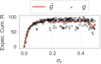
In our context, noise corresponds to the difference between the observation $y$ and the expected cumulative reward for a given setting ${\boldsymbol{\mathbf{x}}}$, i.e. $\nu({\boldsymbol{\mathbf{x}}}):=y-\hat{g}({\boldsymbol{\mathbf{x}}})$. Recalling Sec. III-C, $\nu({\boldsymbol{\mathbf{x}}})$ can be modelled as an independent zero-mean Gaussian process with covariance function $k_{\nu}$. We consider episodes to be executed independently, so that $k_{\nu}({\boldsymbol{\mathbf{x}}},{\boldsymbol{\mathbf{x}}}^{\prime})=0$ for ${\boldsymbol{\mathbf{x}}}\neq{\boldsymbol{\mathbf{x}}}^{\prime}$. Our concern is then modelling $k_{\nu}({\boldsymbol{\mathbf{x}}},{\boldsymbol{\mathbf{x}}})=\sigma_{\nu}^{2}({\boldsymbol{\mathbf{x}}})$.

In this paper, we assume a flexible parametric form for the noise model:

where ${\boldsymbol{\mathbf{\beta}}}\in\mathbb{{R}}^{m}$, $\zeta\geq 0$ and ${\boldsymbol{\mathbf{\phi}}}:{\mathcal{{X}}}\to\mathbb{{R}}^{m}$ is a feature map. A scalar factor $z$ is added to determine variations of the cumulative reward around its expected value. Small values of $z$ produce expected cumulative reward functions that are close to their mean, and larger values allow more variation. If $z$ is large, the modelled expected cumulative reward function will be able to account for more outliers. A smooth feature map $\phi$ allows the noise model to fit the gradually changing noise variance, as in Fig. 4, with no sharp changes across the search space, and the exponential function ensures the positive-definiteness of $k_{\nu}$.

The offset term $\zeta$ accounts for any homoscedastic component in the noise process, representing a minimum amount of noise to expect. The exponential term includes a generalised linear model ${\boldsymbol{\mathbf{\beta}}}^{\mathsf{T}}{\boldsymbol{\mathbf{\phi}}}({\boldsymbol{\mathbf{x}}})$ which allows us to vary the noise distribution as a function of the input. The choice of feature map ${\boldsymbol{\mathbf{\phi}}}$ is arbitrary. For instance, polynomial features allow us to capture general non-linear trends, while kernel-based features allow us to model localised behaviour.

Having a parametric form for $k_{\nu}$, there are multiple methods to learn a suitable noise model from data. In this paper, we deal with two of them. One can either directly maximise the log-marginal likelihood [20] of the GP representing $\hat{g}\sim\mathcal{GP}(m,k)$ alongside other GP hyper-parameters $\theta$ or learn noise parameters separately in a two-stage regression problem, which is described further below.

From a set of randomly sampled inputs ${\boldsymbol{\mathbf{x}}}_{i}\in{\mathcal{{S}}}$, we can approximate the expected reward $\hat{g}$ with the flexible generalised linear regression model based on the feature map ${\boldsymbol{\mathbf{\phi}}}:{\mathcal{{X}}}\to\mathbb{{R}}^{m}$ and learnt weights ${\boldsymbol{\mathbf{\alpha}}}\in\mathbb{{R}}^{m}$ as:

With this estimate $\hat{g}$ we then fit the residuals $q({\boldsymbol{\mathbf{x}}}):=|g({\boldsymbol{\mathbf{x}}})-\hat{g}({\boldsymbol{\mathbf{x}}})|$ with (9) as a regression problem.

We optimise the controller with BO, a global optimisation method, by maximising the episodic or cumulative reward $g$ dependent on controller hyper-parameters ${\boldsymbol{\mathbf{x}}}$ to solve ${\boldsymbol{\mathbf{x}}}^{*}=\operatornamewithlimits{argmax}g({\boldsymbol{\mathbf{x}}})$. Considering $g$ is stochastic, we maximise the expected cumulative reward $\hat{g}_{t}=\mathbb{E}\left[g({\boldsymbol{\mathbf{x}}}_{t})\right]$.

The controller hyper-parameters are optimised following Algorithm 2. At each BO iteration, we fit the GP model $\mathcal{M}$ with observations collected up to the current iteration $t$. Next, we select controller hyper-parameters ${\boldsymbol{\mathbf{x}}}_{t}$ by maximising the acquisition function $h$ with a global optimisation method. We then compute the expected cumulative reward $\hat{g}_{t}$ empirically by averaging the cumulative rewards obtained after $n_{r}$ episodes of $n_{e}$ time steps each. At each time-step $i$, an optimal action $a^{*}_{i}$ is returned by the MPC controller configured with ${\boldsymbol{\mathbf{x}}}$ and sent to the system actuators. This returns a reward $r_{i}$ that is accumulated in $g_{j}({\boldsymbol{\mathbf{x}}}_{t})$, where $j$ is the current repetition. Finally, the optimal controller hyper-parameters ${\boldsymbol{\mathbf{x}}}^{*}$ correspond to those with maximum expected cumulative after $n_{BO}$ optimisation iterations.

We conducted experiments on benchmark control problems from OpenAI Gym¹¹ 1 OpenAI Gym: https://gym.openai.com [27] and Mujoco [28]: Acrobot, Cartpole, Half-Cheetah, Pendulum, and Reacher.

Each control problem has a particular state reward function $r({\boldsymbol{\mathbf{s}}},\mathbf{a})$ shown in Table I. We made slight modifications in Reacher and Half-Cheetah. We reduced the effect of actions and gave more priority to the distance to the target in the case of the Reacher problem. For Half-Cheetah, we added more priority to the inclination, since Half-Cheetah would tend to turn upside down as its speed increases. The actuation is then set to finish when such inclination is greater than $\pi/2$ or lower than $-\pi/2$. These modifications make the rewards more informative for MPPI, enabling it to solve these two tasks. We can then focus the analysis on tuning the controller.

The expected cumulative reward represents the expected time the pendulum stays in an upright position in the Acrobot, Cartpole, and Pendulum. It represents the distance traversed in Half-Cheetah, and the speed to reach the target in Reacher. High expected cumulative rewards are the result of motions that increased the reward accordingly, e.g. Half-Cheetah would be expected to reach farther distances.

Now, to evaluate the expected cumulative rewards for each problem, we determined fixed values for time horizon $T$, number of trajectory rollouts $M$, and MPPI hyper-parameter intervals are shown in Table II. These were found by narrowing down large-enough intervals from near-zero values to 500, taking into account usual values for these hyper-parameters that tend to be close to 0. These are typical in several applications [18, 17]. The table also shows optimal values found within these narrowed intervals via grid search.

For better comparison, both BO variations were implemented using the same squared exponential kernel $k(x,x^{\prime})=\sigma_{n}^{2}\exp\left(-\frac{(x-x^{\prime})^{2}}{2\ell^{2}}\right)$ and UCB acquisition function from (7) with $\kappa=1.2$. For the optimisation of the acquisition function $h$ we used L-BFGS-B [30] with random starting points as a global optimisation method. We also maximised the marginal likelihood to find the GP hyper-parameters $\theta:=\{\sigma,\sigma_{n},\ell\}$ for BO_homo and $\theta:=\{z,\sigma_{n},\ell\}$ for BO_hetero also using L-BFGS-B. $\theta$ was kept fixed after it was optimised.

Both BO variations were optimised by maximising the GP marginal likelihood of previously observed sample points, which were generated from the defined hyper-parameter intervals from Table II for each problem.

A polynomial basis function ${\boldsymbol{\mathbf{\phi}}}$ was used for BO_hetero and evaluated for different degrees. A polynomial degree of 1 as in Fig. 6a and 5 as in Fig. 6b would result in a noise model ignoring small variances while a higher degree would not. We then set a 10-degree polynomial model Fig. 6c because it is the first high degree that correctly handles the increasing variance.

The noise model was computed using the regression model in (10). Something else to note about the GP hyper-parameters is that their values have to be proportional to the range of the expected cumulative reward function to model for standard comparison among functions, so the expected cumulative rewards were scaled to $[0,100]$.

In Fig. 5, we visualise and evaluate the varying noise behaviour of the expected cumulative reward for intervals of MPPI hyper-parameters. We can see that the noise around the mean increases with the $x$-axis hyper-parameter. The expected cumulative reward function for varying temperatures $\lambda$ can be seen only in the Acrobot example, as temperature variations were not significant in the rest of the problems.

The noise heteroscedasticity is evident in all the control problems, so we answer Q1. There is a gain over BO_homo as more noise is captured. However, in Half-Cheetah and Pendulum, the noise is quite skewed around the mean, which means that the expected cumulative reward may not be Gaussian in those cases. The framework still captures a Gaussian noise for the rest of the control problems.

To answer Q2, in Fig. 7, we compare BO_hetero, BO_homo, and covariance matrix adaptation evolution strategy (CMA-ES) [31], which is a non-BO baseline that does not take heteroscedasticity into account. To allow for proper comparison, each method started at a single defined point in the search space where there’s a minimum. We use CMA-ES with $\sigma_{0}=1$ and population size of $2$. CMA-ES has been used for hyper-parameter tuning and is considered to be a data-efficient black-box optimiser [32, 33].

As expected, BO_hetero overcomes BO_homo and CMA-ES. For BO_homo, the standard deviation reflects incorrect noise modelled in some regions as also shown in Fig. 5. BO_homo ends up with a higher standard deviation in most cases. In Acrobot and Reacher, we did not find much improvement due to mostly homoscedastic regions in the sample collected.

To assess long-term performance, we let the optimisation continue for 200 iterations for Half-Cheetah in Fig. 8. As BO_hetero describes the overall noise behaviour, it finds optimal regions faster than CMA-ES.

It is important to note that CMA-ES does not run inference from prior data. BO is able to apply prior knowledge encoded in the noise model to outperform CMA-ES in fewer iterations. BO approaches do more global search in fewer trials, which is the desired behaviour for a data-efficient solution.

We experimented optimising Half-Cheetah and Reacher with their unmodified reward functions in Fig. 9. The unmodified reward functions make the tasks difficult to all methods, which suggests MPPI has difficulties in solving these tasks. A possible reason is that the unmodified cost function is too uninformative for the MPPI controller.

To assess the effects of real heteroscedastic noise in a physical system, we performed experiments on tuning an MPPI controller for a physical robot. The four-wheel-drive skid-steer robot (Fig. 10a) was tasked with following a circular path at a set speed. The cost function was formulated as $c(s_{t})=\sqrt{d_{t}^{2}+(v_{r}-v_{t})^{2}}$, where $d_{t}$ represents the robot’s distance to the edge of the circle, $v_{r}=0.2$ m/s is a reference linear speed, and $v_{t}$ is the current speed. The robot was localised using a particle filter on a prebuilt map. Internally, MPPI employed a kinematic model of the robot [34] for trajectory rollouts which is challenging for MPC as the model does not simulate the dynamics of skid-steering platforms accurately. The controller was configured with $M=50$ rollouts and a time horizon $T=400$. Episodes lasted 20 seconds with the robot starting from a fixed initial position. The search space ${\mathcal{{S}}}$ for BO was set as the box defined by the intervals $\sigma_{\epsilon}\in[0.3,0.5]$ and $\lambda\in[0.01,0.21]$.

Fig. 10bpresents the learnt heteroscedastic noise model. Data from preliminary runs revealed that the noise in the episode rewards had a concentrated region of high-variance in roughly the middle of the search space. As previously discussed, both the temperature $\lambda$ and the control noise variance $\sigma_{\epsilon}^{2}$ influence MPPI’s exploration-exploitation trade-off. For this experiment, the bounds for $\sigma_{\epsilon}$ were chosen as settings that lead to acceptable performance in practice, but we allowed for a $\lambda$ range which could cause instability. High temperatures $\lambda$ cause excessive exploration in the action space of MPPI, which leads to an almost-sure failure in execution. Conversely, low temperatures force MPPI to take actions that are close to optimal, leading to mostly high rewards. The middle ground between temperature extremes, however, is the region where behaviour is unstable. MPPI’s control variance $\sigma_{\epsilon}^{2}$ contributes to this behaviour in a similar fashion by determining the spread of the exploration.

To appropriately model the aforementioned noise concentration behaviour, we set the GP noise model as a mixture of stationary kernels by defining (cf. (9)):

where the coefficients $\zeta\in\mathbb{{R}}$, the weights ${\boldsymbol{\mathbf{\beta}}}\in\mathbb{{R}}^{m}$ and the points ${\boldsymbol{\mathbf{x}}}_{i}\in{\mathcal{{S}}}$, alongside the other GP hyper-parameters, were tuned offline by maximum a posteriori estimation²² 2 As reasonable choices for the priors, we set log-Gaussian priors for positive GP hyper-parameters and Gaussian priors for the rest.. As kernel $k_{q}$, we used the rational quadratic kernel [20, p. 87].

Performance results are in Fig. 10c. We compared BO_hetero against BO_homo. Both algorithms are eventually able to find high reward regions. However, due to its uniform noise model, BO_homo is led to a more exploratory behaviour, instead of concentrating on promising regions, as evidenced by the query locations in Fig. 11. As a consequence, we observe a significant drop in performance during the optimisation, as shown in Fig. 10c. In contrast, BO_hetero maintains a steady high performance, which means lower tracking error with respect to the circular path specified by the cost function.

References

- [1] T. M. Howard, C. J. Green, and A. Kelly, “Receding Horizon Model-Predictive Control for Mobile Robot Navigation of Intricate Paths,” Field and Service Robotics, vol. 62, pp. 69–78, 2010.
- [2] B. Paden, M. Cap, S. Z. Yong, D. Yershov, and E. Frazzoli, “A Survey of Motion Planning and Control Techniques for Self-Driving Urban Vehicles,” IEEE Transactions on Intelligent Vehicles, vol. 1, no. 1, pp. 33–55, 2016.
- [3] G. Williams, N. Wagener, B. Goldfain, P. Drews, J. M. Rehg, B. Boots, and E. A. Theodorou, “Information theoretic MPC for model-based reinforcement learning,” in Proceedings of the IEEE International Conference on Robotics and Automation, 2017, pp. 1714–1721.
- [4] J. B. Rawlings, D. Q. Mayne, and M. M. Diehl, Model predictive control: Theory, Computation, and Design. Madison, WI, USA: Nob Hill Publishing, 2017, vol. 197.
- [5] G. Williams, A. Aldrich, and E. A. Theodorou, “Model predictive path integral control: From theory to parallel computation,” Journal of Guidance, Control, and Dynamics, vol. 40, no. 2, pp. 344–357, 2017.
- [6] B. Shahriari, K. Swersky, Z. Wang, R. P. Adams, and N. De Freitas, “Taking the human out of the loop: A review of Bayesian optimization,” Proceedings of the IEEE, vol. 104, no. 1, pp. 148–175, 2016.
- [7] S. Kuindersma, R. Grupen, and A. Barto, “Variational Bayesian Optimization for Runtime Risk-Sensitive Control,” in Robotics: Science and Systems (RSS), Sydney, Australia, 2012.
- [8] A. Wilson, A. Fern, and P. Tadepalli, “Using Trajectory Data to Improve Bayesian Optimization for Reinforcement Learning,” Journal of Machine Learning Research, vol. 15, pp. 253–282, 2014.
- [9] M. W. Spong, “The swing up control problem for the acrobot,” IEEE Control Systems Magazine, vol. 15, no. 1, pp. 49–55, Feb 1995.
- [10] T. Wilson and S. B. Williams, “Active sample selection in scalar fields exhibiting non-stationary noise with parametric heteroscedastic Gaussian process regression,” Proceedings of the IEEE International Conference on Robotics and Automation, pp. 6455–6462, 2017.
- [11] D. Görges, “Relations between Model Predictive Control and Reinforcement Learning,” IFAC-PapersOnLine, vol. 50, no. 1, pp. 4920–4928, 2017.
- [12] M. P. Deisenroth, “A Survey on Policy Search for Robotics,” Foundations and Trends in Robotics, vol. 2, no. 1-2, 2013.
- [13] K. Chua, R. Calandra, R. McAllister, and S. Levine, “Deep Reinforcement Learning in a Handful of Trials using Probabilistic Dynamics Models,” in Advances in Neural Information Processing Systems, 2018, pp. 4754–4765.
- [14] A. R. Mahmood, D. Korenkevych, G. Vasan, W. Ma, and J. Bergstra, “Benchmarking Reinforcement Learning Algorithms on Real-World Robots,” in 2nd Conference on Robot Learning (CoRL 2018), Zurich, Switzerland, 2018.
- [15] A. S. Polydoros and L. Nalpantidis, “Survey of Model-Based Reinforcement Learning: Applications on Robotics,” Journal of Intelligent and Robotic Systems: Theory and Applications, vol. 86, no. 2, pp. 153–173, 2017.
- [16] T. Wang, X. Bao, I. Clavera, J. Hoang, Y. Wen, E. Langlois, S. Zhang, G. Zhang, P. Abbeel, and J. Ba, “Benchmarking Model-Based Reinforcement Learning,” Arxiv, 2019.
- [17] G. Williams, P. Drews, B. Goldfain, J. M. Rehg, and E. A. Theodorou, “Aggressive driving with model predictive path integral control,” Proceedings of the IEEE International Conference on Robotics and Automation, vol. 2016-June, pp. 1433–1440, 2016.
- [18] C. Liang, W. Wang, Z. Liu, C. Lai, and B. Zhou, “Learning to Guide: Guidance Law Based on Deep Meta-Learning and Model Predictive Path Integral Control,” IEEE Access, vol. 7, pp. 47 353–47 365, 2019.
- [19] J. Snoek, H. Larochelle, and R. Adams, “Practical Bayesian Optimization of Machine Learning Algorithms,” in Advances in Neural Information Processing (NIPS), 2012.
- [20] C. E. Rasmussen and C. K. I. Williams., Gaussian Processes for Machine Learning. The MIT Press, 2006.
- [21] P. W. Goldberg, C. K. Williams, and C. M. Bishop, “Regression with input-dependent noise a Gaussian process treatment,” in Advances in Neural Information Processing Systems, 1998, pp. 493–499.
- [22] C. Andrieu, N. De Freitas, A. Doucet, and M. I. Jordan, “An introduction to MCMC for machine learning,” Machine Learning, vol. 50, no. 1-2, pp. 5–43, 2003.
- [23] K. Kersting, C. Plagemann, P. Pfaff, and W. Burgard, “Most likely heteroscedastic Gaussian process regression,” ACM International Conference Proceeding Series, vol. 227, pp. 393–400, 2007.
- [24] M. Lázaro-Gredilla and M. K. Titsias, “Variational heteroscedastic Gaussian process regression,” in Proceedings of the 28th International Conference on Machine Learning, ICML 2011, 2011, pp. 841–848.
- [25] G. Williams, P. Drews, B. Goldfain, J. M. Rehg, and I. A. Theodorou, “Information-Theoretic Model Predictive Control: Theory and Applications to Autonomous Driving,” IEEE Transactions on Robotics, vol. 34, no. 6, pp. 1603–1622, 2018.
- [26] D. D. Cox and S. John, “A statistical method for global optimization,” in Proceedings of the IEEE International Conference on Systems, Man and Cybernetics, vol. 1992-Janua, 1992, pp. 1241–1246.
- [27] G. Brockman, V. Cheung, L. Pettersson, J. Schneider, J. Schulman, J. Tang, and W. Zaremba, “OpenAI Gym,” Arxiv, 2016.
- [28] E. Todorov, T. Erez, and Y. Tassa, “MuJoCo: A physics engine for model-based control,” in IEEE International Conference on Intelligent Robots and Systems, 2012, pp. 5026–5033.
- [29] J. R. Gardner, C. Guo, K. Q. Weinberger, R. Garnett, and R. Grosse, “Discovering and exploiting additive structure for Bayesian optimization,” in Proceedings of the 20th International Conference on Artificial Intelligence and Statistics, AISTATS 2017, vol. 54, 2017.
- [30] R. H. Byrd, P. Lu, J. Nocedal, and C. Zhu, “A limited memory algorithm for bound constrained optimization,” SIAM Journal on scientific computing, vol. 16, no. 5, pp. 1190–1208, 1995.
- [31] D. V. Arnold and N. Hansen, “Active covariance matrix adaptation for the (1+1)-CMA-ES,” in Proceedings of the 12th annual conference on Genetic and evolutionary computation - GECCO ’10. Portland, OR: ACM, 2010, p. 385.
- [32] I. Loshchilov and F. Hutter, “Cma-es for hyperparameter optimization of deep neural networks,” arXiv preprint arXiv:1604.07269, 2016.
- [33] J. Karro, “Black Box Optimization via a Bayesian-Optimized Genetic Algorithm,” in Conference on Neural Information Processing Systems, 2017.
- [34] K. Kozlowski and D. Pazderski, “Modeling and control of a 4-wheel skid-steering mobile robot,” International Journal of Applied Mathematics and Computer Science, vol. 14, no. 4, pp. 477–496, 2004.