Truly Subquadratic Exact Distance Oracles with Constant Query Time for Planar Graphs
Abstract
Given an undirected, unweighted planar graph with vertices, we present a truly subquadratic size distance oracle for reporting exact shortest-path distances between any pair of vertices of in constant time. For any , our distance oracle takes up space and is capable of answering shortest-path distance queries exactly for any pair of vertices of in worst-case time . Previously no truly sub-quadratic size distance oracles with constant query time for answering exact all-pairs shortest paths distance queries existed.
1 Introduction
Efficiently answering shortest path distance queries between pairs of vertices in a graph is a fundamental algorithmic problem with numerous important applications. Given an -vertex graph a distance oracle is a compact data-structure capable of efficiently answering shortest path distance queries between pairs of vertices . Ideally one would like the data structure to be of linear size and the query time to be constant. However, it is well known that there are graphs for which no distance oracle with bits of space and query time exists. In fact, even resorting to approximation, Pǎtraşcu and Roditty [20] showed that there are sparse graphs on edges for which constant query-time distance oracles with stretch less than must be of size , assuming the set intersection conjecture. These impossibility results make it natural to consider the probelms in restricted classes of graphs.
In this paper we consider exact distance oracles for planar graphs. Distance oracles for planar graphs are well motivated by important real-world applications, notably in routing, navigation of road and sea maps as well as in the context of computational geometry. To the best of our knowledge there are no non-trivial lower bounds for (static) distance oracles for planar graphs, and thus achieving the “holy grail” of a linear-size distance oracle with constant query time may be possible. Indeed, there has been numerous works over at least three decades developing exact distance oracles for planar graph [10, 2, 3, 8, 11, 18, 19]. However, only recently Cohen-Addad et al. [9] gave the first oracle with truly subquadratic space and polylogarithmic query time. Their result was inspired by Cabello’s [4] breakthrough result, who gave the first truly sub-quadratic time algorithm for computing the diameter of planar graphs by a novel use of Voronoi diagrams. The approach of [9] was subsequently improved by [12, 7], who gave an elegant point-location mechanism for Voronoi diagrams in planar graphs, and combined it with a clever recursive scheme to obtain exact distance oracles for directed weighted planar graphs with space and query time for any small constant . We note that even though the oracle of [7] gets quite close to optimal, it remains wide open to support exact queries in constant time using truly subquadratic space, even in the most basic case of unweighted undirected planar graphs [25, 5, 24].
Allowing approximate answers does help in planar graphs. Many results reporting -approximate distances with various tradeoffs exist, all with (nearly) linear size and polylogarithmic, or even query-time [23, 15, 14, 26]. Gu and Xu[13] presented a size distance oracle capable of reporting -approximate distances in time . While their query time is a constant independent of , the preprocessing time and space are nearly linear, but with an exponential dependency on . This exponential dependency was recently improved to polynomial [6].
Thus, despite the large body of work on distance oracles for planar graphs, it has remained an open question to determine whether an exact distance oracle with of size with constant query-time can be constructed for some constant .
Our results and techniques.
We answer this question in the affirmative. Our result is presented in the following theorem:
Theorem 1.
Let be an undirected unweighted -vertex planar graph. For any there exists a data-structure requiring space that, for any , reports the shortest path distance between and in in time .
We remark that the simple distance oracle we present in Section 4 can be distributed into a distance labeling scheme with size per label, such that the distance between any two vertices can be computed in time given just the labels of and .
The main concept we use to obtain our result is that of a pattern capturing distances between a vertex and a cycle. This concept was used by [25] , and weas called “distance tuple” by and [17]. Consider a vector storing the distances from a vertex to the vertices of a cycle in their cyclic order. The pattern of w.r.t. is simply the discrete derivative of this vector. That is, the vector obtained by taking the difference between every pair of consecutive values. Li and Parter [17] observed that when the input graph is planar, the number of different patterns w.r.t. a face with vertices is regardless of the size of the graph. We next outline how this observation can be used to break the quadratic space barrier.
Roughly speaking, any planar graph can be decomposed into subgraphs, called regions, of size each, where the boundary of each region (i.e., the vertices that have neighbors outside the region) is a single cycle .11 1 In fact, a constant humber of cycles. To readers familiar with the concept, this is just an -division with a few holes, but without the important feature that each region has just boundary vertices. This is because one cannot triangulate unweighted graphs without changing the distances. Applying Li and Parter’s observation in this setting, the number of different patterns for the hole of each region is . Hence, we can represent the distances from any vertex to by just storing the distance from to an arbitrarily chosen canonical vertex of , and a pointer to the pattern of with respect to . This requires just space plus for storing all the patterns for . Summing over all regions, the space required is . We define the notion of distance from a pattern to a vertex (see Definition 2). While this definition is simple, it is somewhat unnatural because the distance from a pattern to a vertex does not necessarily correspond to the length of any specific path in the graph! However, the distance between and any vertex is just the sum of the distance between and the canonical vertex and the distance from the pattern of with respect to to .
We therefore store the distances from each of the possible patterns of to each vertex of . This requires space per region, so space overall. This way we can report the distance between and in constant time by (i) retrieving the pattern of w.r.t. , and (ii) adding the distance from to the canonical vertex of and the distance from the pattern to . These ideas alone already imply an oracle with space and constant query time. Combining these ideas with recursion yields the improved space bound of Theorem 1.
As we argued in the introduction, breaking the quadratic space barrier for constant query time is important and significant result in its own right. We highlight the following difference between the approach taken in our recursive oracle and the approaches used in all existing distance oracles we are aware of. To the best of our knowledge, all existing distance oracles, both exact and approximate, and both for general graphs and planar graphs, recover the distance from to by identifying a vertex or vertices on some (possibly approximate) shortest path between and , for which distances have been stored in the preprocessing stage. These vertices are usually referred to as landmarks, portals, hubs, beacons, seeds, or transit nodes [22]. Our oracle, on the other hand, reports the exact shortest path without identifying vertices on the shortest path from to . Instead, it ”zooms in” on by recovering distances to the canonical vertices of a sequence of subgraphs of decreasing size that terminates at a constant size graph containing . We emphasize that none of these canonical vertices necessarily lies on a shortest path from to . This property may be viewed as a disadvantage if we also want to report the shortest path, but when reporting multiple edges on long paths, constant query time is no longer relevant. On the other hand, it may be that just reporting the distance is easier than also reporting an internal vertex on a shortest path. Hence, it may be that developing oracles based on this new approach may lead to further advances on the way to linear size distance oracles for planar graphs with constant query time, and in other related problems.
2 Preliminaries
Let be a graph. We denote by and the vertex and edge-set of , and denote by the number of vertices of . For a subset of edges or vertices we denote by the subgraph of induced on . We denote by a shortest path from to in the subgraph , by the length of , and define .
The following definitions will be useful when talking about decompositions of . A region of is an edge-induced subgraph of , and its boundary is the vertices of that are adjacent to some vertex of in . Vertices of are called interior vertices of . Observe that for a region and for and , any path from to in must intersect .
It will be useful to assume some global strict order on a vertex set s.t. for any there is a minimum vertex w.r.t this order. We refer to this as the canonical vertex of .
Faces and holes:
We assume the reader is familiar with the the basic definitions of planarity and of planar embeddings. The edges of a plane graph induce maximal open portion of the plane that do not intersect any edges. A face of the graph is the closure of one such portion of the plane. We refer to the edges bounding a face as the boundary of that face. Given a face , is the set of vertices on the boundary of . We denote by the facial walk of which is the sequence of vertices encountered when walking along starting at and going in the clockwise direction. Note that may be non-simple, so some vertices may appear multiple times in .
A hole in a region of a graph is a face of which is not a face in . We say that a vertex is inside hole if lies in the region of the plane corresponding to the face of . We denote by all the vertices that are inside .
Decompositions of unweighted planar graphs.
An -division is a widely used decomposition of planar graphs into regions with small boundary. We use the -divisions with a few holes as studied in [16], which works for triangulated biconnected graphs:
Lemma 1.
(-division with few holes for triangulated graphs [16]) Let be a biconnected, triangulated -vertex planar embedded graph, and let . can be decomposed into connected regions, each of which with vertices and boundary vertices. Each region has a constant number of holes. Every boundary vertex lies on some hole, and each hole has vertices.
The fact that the boundaries of regions are small (only boundary vertices for a region with vertices) is the basis for many efficient algorithms and data structures for planar graphs. Unweighted planar graphs posses additional structure (in comparison to weighted planar graphs), which may also be useful algorithmically. See for example the unit-Monge property in [1], or the limited number of patterns [25, 17], which we use in this work. However, exploiting such additional structure in conjunction with a decomposition into regions with small boundaries has been elusive because of the seemingly technical requirement in Lemma 1 that the graph be triangulated and biconnected.
Any graph can be triangulated and biconnected by adding to each face an artificial vertex and infinitely weighted artificial edges from the artificial vertex to each vertex of . This transformation preserves planarity and shortest paths, and ensures that the graph consists only of simple faces of size 3. However, the graph is no longer unweighted. We refer to an artificial vertex (edge) of as a vertex (edge) which was added in the triangulation step, and a natural vertex (edge) of as a vertex (edge) which is not artificial. In order to exploit the structure of the unweighted input graph we will remove the artificial edges and vertices after computing the decomposition using Lemma 1. On the one hand the graph is again unweighted. On the other hand, while the number of boundary vertices in each region remains , the holes may now contain new non-boundary vertices, and the total size of the holes in each region may be . We note, however, that the deletion of artificial edges and vertices does not disconnect regions [16]. We therefore restate the decomposition lemma for unweighted graphs that are not necessarily triangulated or biconnected.
Lemma 2.
(-division with few holes for non-triangulated graphs) Let be a -vertex planar embedded graph , and let . can be decomposed into connected regions, each of which with vertices and boundary vertices. Each region has a constant number of holes, and each boundary vertex lies on some hole.
Recursive -divisions.
Our second construction relies on a recursive -division which is a recursive decomposition of into -divisions for varying values of . Specifically, for a decreasing sequence , where , we want -divisions for all , such that each region in the division is the union of regions in the -division on the next level. We associate with the recursive -division a decomposition tree, , which is a rooted tree whose nodes correspond to the regions of the recursive decomposition of . We will refer to nodes and their corresponding regions interchangeably. The root node corresponds to all of . A node of at depth corresponds to a region of the -division, and its children are the regions of the -division whose union is the region corresponding to . We denote by all the nodes at level . It was shown in [16] that recursive -divisions can be computed efficiently:
Lemma 3.
(Recursive -division) Given a biconnected, triangulated -vertex planar graph and an exponentially decreasing sequence , a decomposition tree, can be computed in linear time s.t corresponds to an -division of with few holes for each .
3 Patterns
Both [25] and [17] introduce a notion of a “distance tuple” which can be thought of as a vector of shortest-path distances from a vertex to consecutive vertices of some hole. We introduce the following similar notion of a pattern (See Figure 1 for an illustration):
Definition 1.
(Pattern) Let be a graph. Let be a subgraph of . Let be a vertex in , and let be a path in . The pattern of (w.r.t. in ) is a vector satisfying for . For a region in , a hole of , and a vertex , we write instead of .
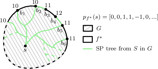
Definition 2.
(pattern to vertex distance) Let be a region in a graph . Let be a hole of . Let be the vertices of in their cyclic order. Let be some pattern w.r.t. (i.e., for some ). For a vertex we define the distance between and to be .
Lemma 4.
Let be a region of a graph . Let be a hole of . For every and every , .
Proof.
By definition of pattern and by a telescoping sum, for every , . Let be any vertex of on a shortest -to- path ( exists since and ). By choice of , . ∎
Bounding the number of patterns
As mentioned, In a recent paper, Li and Parter [17] achieve improved bounds for diameter computation for planar graphs by showing that in unweighted undirected planar graphs the number of patterns is quite small. More specifically, they show that the VC-dimension of a set corresponding to all patterns is at most 3. By the Sauer-Shelah lemma [21], this implies that the number of distinct patterns w.r.t. a face is in . Their result is stated in the following lemma:
Lemma 5.
(Pattern compression) [17] Let be an -vertex unweighted undirected planar graph, let be a face in , and let be a set of consecutive vertices on . Then the number of distinct patterns w.r.t. , , is bounded by .
We observe that the bound of Lemma 5 also holds for patterns w.r.t. the entire set of vertices on a hole of a region even when distances are defined in the entire graph .
Corollary 1.
Let be a region in an -vertex unweighted undirected planar graph , and let be a hole of . Then the number of distinct patterns w.r.t. , , is bounded by .
Proof.
Since is a hole of , is a face of . By Lemma 5, . The corollary follows since for every two vertices , implies . ∎
For the remainder of the paper we only deal with distances in and with patterns in , so we will omit the subscript , and write and instead of and .
4 space distance oracle
Before presenting our main result, we describe a simpler construction which yields a distance oracle with a larger space requirement of and query time:
Preprocessing.
The preprocessing consists of computing an -division of with a parameter to be determined later. For every vertex of and every region of , we store the hole of s.t. is in . This requires space.
For every region , for every hole of , we maintain the patterns of the vertices in w.r.t. as follows. Let denote the size of the boundary walk of . let be the canonical (i.e., first) vertex of . We maintain the patterns seen so far in a ternary tree whose edges are labeled by . The depth of is , and the labels along each root-to-leaf path correspond to a unique pattern, which we associate with that leaf. For every vertex , we compute the pattern and we make sure that is represented in the tree by adding the corresponding labeled edges that are not yet present in . After all the vertices in were handled, the tree has leaves. For each leaf of with an associated pattern , we compute and store (i) the distance from to each vertex of . This requires time and space for all leaves of , so a total of space for storing all this information over all regions.
For each vertex we store (ii) a pointer to (the leaf of that is associated with) the pattern , as well as (iii) the distance between and the canonical vertex of . The total space required to store all these pointers and distances is .
To complete the preprocessing we also store (iv) for each region , the distance for all pairs of vertices . This takes additional space, which is dominated by the above terms.
The total space required by the oracle is thus . This is minimized for , resulting in an -space data structure.
We note that once this information has been computed we no longer need to store the entire tree . Rather, it suffices to only store just the list of leaves of and the distances stored with each of them. In particular, we no longer need to remember what is the actual pattern associated with each leaf, we only need to know the distances from this pattern to the vertices of the region . In the current scheme this has no asymptotic effect on the size of the data structure, since each pattern is of size , and we anyway store the distances from each pattern to all vertices of . However, in the recursive scheme in the next section this observation will become useful.
Query.
To answer a query for the distance between vertices and we proceed as follows. If and are in the same regions, we simply return the distance stored in item (iv). Otherwise, let be the region containing , and let be the hole of such that . Let be the canonical vertex of . We return . The correctness is immediate from Lemma 4. We note that is stored in item (iii), a pointer to is stored in item (ii), and is stored in item (i). The query is illustrated in Figure 2.

As aforementioned this oracle can be distributed into a distance labeling of size per label such that the distance between any two vertices can be computed in time given just the labels of and .
5 space distance oracle
A bottleneck in the above approach comes from having to store, for each pattern of a hole of a region , the distances from to all vertices of . Instead, we use a recursive -division, in which we store for , only the distances to the canonical vertex of a hole of each child region of instead of all the vertices in the region. For this information to be useful we also store the pattern induced by on the hole , which is defined as follows.
Definition 3.
(Pattern induced by a pattern) Let be a region in a graph . Let be a hole of and be a pattern of (w.r.t. a vertex or another pattern). Let be a child region of . Let be the vertices of the boundary walk of a hole of of . The pattern induced by on is the vector satisfying for .
Lemma 6.
Consider the settings of Definition 3. If for some , then .
Proof.
By Lemma 4, for every , . Hence for all , , which is, by definition, . ∎
Preprocessing.
We first compute a -division of for to be determined later, and denote by the associated decomposition tree. For convenience, we let , and define . In the following we let denote the set . We store the following:
- 1.
For each we store a list of regions containing , where . (Recall that is the set of all nodes of at level ).
- 2.
For each , for each , for each region containing , for each child region at level-, let be the hole of such that . We associate with the pair (i) a pointer to , (ii) the canonical vertex , and (ii) the distance .
- 3.
For each , for each , for each hole in , for each and for each , let be the hole of such that . We associate with the pair (i) a pointer to the pattern induced by on , (ii) the canonical vertex , and (iii) the distance .
Space analysis.
Storing 1 requires space . To bound the space for item 2, we note that the number of regions at level to which a vertes belongs is bounded by the degree of . Since the average vertex degree in a planar graph is at most 6, the average number of regions at level to which belongs is at most 6. Each such region has subregions at level-, so storing 2 requires space . Storing 3 requires space . The total space is thus, .
Query.
Algorithm 1 show pseudocode describing the query procedure. To process a query the query procedure first determines the largest value for which and belong to the same region in . Note that such a region must always exists as the root of is all of . This level can be found in time by traversing , starting from a leaf region containing and a leaf region containing .
Let be the level- region stored for in item 1. Note that, , and, by choice of , . Hence, is in some hole of . We retrieve the pattern and the distance associated with in item 2. We then proceed iteratively ”zooming” into increasingly smaller regions containing .
We show that the algorithm maintains the invariant that, at the beginning of each iteration, we have a level- region containing , the variable stores , where is the hole of such that , and the variable stores (a pointer) to the pattern . Thus, when we reach the singleton region containing , the variable stores .
We have already established that the invariant is maintained just before the loop is entered for the first time. In each iteration of the loop we retrieve , a level- subregion or containing (available in item 1), and retrieve and (associated with the pair in item 3). By Lemma 4, . By Lemma 6, . Hence, after the assignements in Line 9, the invariant is restored.
The time complexity of the query is clearly .
Choosing parameters:
Recall that the space requirement is . Picking each s.t. results in when , and in a query time of . Choosing , the total space used becomes
for a suitable choice of .
One can decrease the sizes of regions more aggressively to get the query time of of Theorem 1. To this end we choose such that , and . Then the space requirement is . It is not hard to verify that one gets , so with .
References
- [1] A. Abboud, P. Gawrychowski, S. Mozes, and O. Weimann. Near-Optimal Compression for the Planar Graph Metric. In Proceedings of the Twenty-Ninth Annual ACM-SIAM Symposium on Discrete Algorithms, pages 530–549. Society for Industrial and Applied Mathematics, Philadelphia, PA, jan 2018.
- [2] S. Arikati, D. Z. Chen, L. P. Chew, G. Das, M. Smid, and C. D. Zaroliagis. Planar spanners and approximate shortest path queries among obstacles in the plane. In J. Diaz and M. Serna, editors, Algorithms — ESA ’96, pages 514–528, Berlin, Heidelberg, 1996. Springer Berlin Heidelberg.
- [3] S. Cabello. Many Distances in Planar Graphs. Algorithmica, 62(1-2):361–381, feb 2012.
- [4] S. Cabello. Subquadratic Algorithms for the Diameter and the Sum of Pairwise Distances in Planar Graphs. ACM Transactions on Algorithms, 15(2):1–38, dec 2018.
- [5] T. M. Chan. All-pairs shortest paths for unweighted undirected graphs in o(mn) time. ACM Trans. Algorithms, 8(4):34:1–34:17, 2012.
- [6] T. M. Chan and D. Skrepetos. Faster Approximate Diameter and Distance Oracles in Planar Graphs. Algorithmica, 81(8):3075–3098, aug 2019.
- [7] P. Charalampopoulos, P. Gawrychowski, S. Mozes, and O. Weimann. Almost optimal distance oracles for planar graphs. In Proceedings of the 51st Annual ACM SIGACT Symposium on Theory of Computing, STOC 2019, pages 138–151, New York, NY, USA, 2019. Association for Computing Machinery.
- [8] D. Z. Chen and J. Xu. Shortest path queries in planar graphs. In Proceedings of the Thirty-Second Annual ACM Symposium on Theory of Computing, STOC 2000, pages 469–478, New York, NY, USA, 2000. Association for Computing Machinery.
- [9] V. Cohen-Addad, S. Dahlgaard, and C. Wulff-Nilsen. Fast and Compact Exact Distance Oracle for Planar Graphs. In 2017 IEEE 58th Annual Symposium on Foundations of Computer Science (FOCS), pages 962–973. IEEE, oct 2017.
- [10] H. Djidjev. On-line algorithms for shortest path problems on planar digraphs. In Proceedings of the 22nd International Workshop on Graph-Theoretic Concepts in Computer Science, WG 1996, pages 151–165, Berlin, Heidelberg, 1996. Springer-Verlag.
- [11] J. Fakcharoenphol and S. Rao. Planar graphs, negative weight edges, shortest paths, and near linear time. Journal of Computer and System Sciences, 72(5):868–889, aug 2006.
- [12] P. Gawrychowski, S. Mozes, O. Weimann, and C. Wulff-Nilsen. Better tradeoffs for exact distance oracles in planar graphs. In Proceedings of the Twenty-Ninth Annual ACM-SIAM Symposium on Discrete Algorithms, SODA 2018, pages 515–529, USA, 2018. Society for Industrial and Applied Mathematics.
- [13] Q. Gu and G. Xu. Constant query time -approximate distance oracle for planar graphs. In 26th ISAAC, pages 625–636, 2015.
- [14] K.-i. Kawarabayashi, P. N. Klein, and C. Sommer. Linear-Space Approximate Distance Oracles for Planar, Bounded-Genus, and Minor-Free Graphs. apr 2011.
- [15] P. Klein. Preprocessing an undirected planar network to enable fast approximate distance queries. In Proceedings of the Thirteenth Annual ACM-SIAM Symposium on Discrete Algorithms, SODA ’02, pages 820–827, USA, 2002. Society for Industrial and Applied Mathematics.
- [16] P. N. Klein, S. Mozes, and C. Sommer. Structured recursive separator decompositions for planar graphs in linear time. In Proceedings of the 45th annual ACM symposium on Symposium on theory of computing - STOC ’13, page 505, New York, New York, USA, 2013. ACM Press.
- [17] J. Li and M. Parter. Planar diameter via metric compression. In Proceedings of the 51st Annual ACM SIGACT Symposium on Theory of Computing, STOC 2019, pages 152–163, New York, NY, USA, 2019. Association for Computing Machinery.
- [18] S. Mozes and C. Sommer. Exact distance oracles for planar graphs. In Proceedings of the Twenty-Third Annual ACM-SIAM Symposium on Discrete Algorithms, SODA 2012, pages 209–222, USA, 2012. Society for Industrial and Applied Mathematics.
- [19] Y. Nussbaum. Improved distance queries in planar graphs. In Proceedings of the 12th International Conference on Algorithms and Data Structures, WADS 2011, pages 642–653, Berlin, Heidelberg, 2011. Springer-Verlag.
- [20] M. Pǎtraşcu and L. Roditty. Distance Oracles beyond the Thorup–Zwick Bound. SIAM Journal on Computing, 43(1):300–311, jan 2014.
- [21] N. Sauer. On the density of families of sets. Journal of Combinatorial Theory, Series A, 13(1):145–147, jul 1972.
- [22] C. Sommer. Shortest-path queries in static networks. ACM Computing Surveys, 46(4):1–31, apr 2014.
- [23] M. Thorup. Compact oracles for reachability and approximate distances in planar digraphs. Journal of the ACM (JACM), 51(6):993–1024, nov 2004.
- [24] C. Wulff-Nilsen. Algorithms for Planar Graphs and Graphs in Metric Spaces. PhD thesis, 2010.
- [25] C. Wulff-Nilsen. Constant time distance queries in planar unweighted graphs with subquadratic preprocessing time. Computational Geometry, 46(7):831–838, oct 2013.
- [26] C. Wulff-Nilsen. Approximate distance oracles for planar graphs with improved query time-space tradeoff. In Proceedings of the Twenty-Seventh Annual ACM-SIAM Symposium on Discrete Algorithms, SODA ’16, pages 351–362, USA, 2016. Society for Industrial and Applied Mathematics.