Classical Density Functional Theory applied to the solid state

The fundamental quantity in cDFT is the local density $\rho\left(\mathbf{r}\right)$. It is important to emphasize that for an equilibrium system this is identical to the as the one-body probability distribution and as such is a microscopic quantity that involves no coarse-graining or other approximations and, as such, it gives a description of the equilibrium density distribution valid down to the smallest length scales. In cDFT, the local density of an equilibrium system is determined by minimizing a functional denoted here as $\Lambda\left[\rho\right]$. The formal theory underlying cDFT assures us that such a functional exists, that it is unique and that when evaluated at the equilibrium density, it is equal to the grand-canonical free energy of the system, $\Omega$. The ”standard” cDFT model is written as

$$\Lambda\left[\rho\right]=F^{\left(\text{id}\right)}\left[\rho\right]+F^{\left(\text{HS}\right)}\left[\rho\right]+\frac{1}{2}\int\rho\left(\mathbf{r}_{1}\right)\rho\left(\mathbf{r}_{2}\right)w_{att}\left(\mathbf{r}_{1},\mathbf{r}_{2}\right)d\mathbf{r}_{1}d\mathbf{r}_{2}+\int\rho\left(\mathbf{r}\right)\left(\phi\left(\mathbf{r}\right)-\widetilde{\mu}\right)d\mathbf{r}$$

(1)

where the terms are, in sequence, the ideal gas contribution, the hard-sphere contribution, the mean-field contribution and the external field contribution. The ideal-gas part is

$$F^{\left(\text{id}\right)}\left[\rho\right]=k_{B}T\int\left(\rho\left(\mathbf{r}\right)\ln l^{3}\rho\left(\mathbf{r}\right)-\rho\left(\mathbf{r}\right)\right)d\mathbf{r}$$

(2)

where $k_{B}$ is Boltzmann’s constant, $T$ is the temperature and $l$ is any convenient length scale. The next two terms depend on the intermolecular potential which we take to be a pair potential $v\left(r\right)$. This is separated into a repulsive part, $v_{0}\left(r\right)$ and an attractive part $w_{att}\left(r\right)=v\left(r\right)-v_{0}\left(r\right)$. We use the WCA prescription whereby $v_{0}\left(r\right)=v\left(r\right)-v\left(r_{0}\right)$ for $r<r_{0}$ and zero for $r\geq r_{0}$ where $r_{0}$ is the minimum of the potential. Then, an effective hard-sphere diameter $d$ is constructed using any convenient prescription: here, we use the Barker-Henderson recipe

$$d=\int_{0}^{r_{0}}\left(1-e^{-\beta v_{0}\left(r\right)}\right)dr$$

(3)

where $\beta\equiv 1/k_{B}T$. For the hard-sphere contribution, we use the FMT ansatz

$$F^{\left(\text{HS}\right)}\left[\rho\right]=k_{B}T\int\Phi\left(\eta\left(\mathbf{r}\right),s\left(\mathbf{r}\right),\mathbf{v}\left(\mathbf{r}\right)\right)d\mathbf{r}$$

(4)

where the fundamental measures are

$$n^{\left(\alpha\right)}\left(\mathbf{r}\right)=\int w^{\left(\alpha\right)}\left(\mathbf{r-r}^{\prime}\right)\rho\left(\mathbf{r}^{\prime}\right)d\mathbf{r}^{\prime}$$

(5)

with the hard-sphere radius $R=d/2$ and the weights $w^{\left(\eta\right)}\left(\mathbf{r}\right)=\Theta\left(R-r\right)$, $w^{\left(s\right)}\left(\mathbf{r}\right)=\delta\left(R-r\right)$ and $w^{\left(\mathbf{v}\right)}\left(\mathbf{r}\right)=\frac{\mathbf{r}}{r}\delta\left(R-r\right)$ where $\Theta\left(x\right)$ is the step function equal to $1$ if $x>0$ and zero otherwise. Different FMT models are distinguished by the form of the function $\Phi\left(\eta,s,\mathbf{v}\right)$ and here we use the modified RSLT function

$$\Phi\left(\eta,s,\mathbf{v}\right)=-\frac{1}{\pi\sigma^{2}}s\ln(1-\eta)+\frac{1}{2\pi\sigma}\frac{s^{2}-v^{2}}{1-\eta}+\frac{1}{24\pi}\frac{s^{3}\left(1-(v^{2}/s^{2})\right)^{3}}{(1-\eta)^{2}}\phi_{2}(\eta)$$

(6)

with

$$\phi_{2}(\eta)=1-\frac{-2\eta+3\eta^{2}-2(1-\eta)^{2}\ln(1-\eta)}{3\eta^{2}}$$

(7)

which is easily shown to be free of instabilitiesLutsko and Lam 2018. The mean-field term is already given explicitly and we just note that $w_{att}\left(\mathbf{r}_{1},\mathbf{r}_{2}\right)=w_{att}\left(\left|\mathbf{r}_{1}-\mathbf{r}_{2}\right|\right)$, the attractive part of the potential. Finally, $\phi\left(\mathbf{r}\right)$ represents any external one-body field (this plays no role in the present work) and $\widetilde{\mu}=\mu-\ln\left(\frac{\Lambda}{l}\right)^{3}$ where $\mu$ is the chemical potential and $\Lambda$ is the thermal wavelength. The model functional has been presented for a single component system but generalization to multiple components is straightforward.

We discretize the density on a cubic lattice of $N_{x}\times N_{y}\times N_{z}$ points with spacing $\Delta$ and our key approximation is that the density field is approximated by trilinear interpolation of the values of the density at the lattice positions. So, working in units of $\Delta=1$, and defining $\rho_{\mathbf{S}}=\rho\left(S_{x}\widehat{\mathbf{x}}+S_{y}\widehat{\mathbf{y}}+S_{z}\widehat{\mathbf{z}}\right)$ where $S_{x},S_{y},S_{z}$ are integers with $1\leq S_{x}\leq N_{x}$, etc. we write

$$\rho\left(\mathbf{r}\right)=\sum_{\mathbf{I}=0,1}A_{\mathbf{I}}\left(\mathbf{r-S}\left(\mathbf{r}\right)\right)\rho\left(\mathbf{S}\left(\mathbf{r}\right)+\mathbf{I}\right)$$

(8)

where $\mathbf{S}\left(\mathbf{r}\right)$ is the lattice point nearest the origin which is a corner of the computational cell containing the point $\mathbf{r}$, i.e. that for which $\left|S_{x}\right|\leq\left|r_{x}\right|<\left|S_{x}\right|+1$, etc and $\sum_{\mathbf{I}=0,1}$ is shorthand for $\sum_{I_{x}=0,1}\sum_{I_{y}=0,1}\sum_{I_{z}=0,1}$. The coefficients are

$$A_{\mathbf{I}}\left(\mathbf{r}\right)=\left(\delta_{I_{x}0}\left(1-2x\right)+x\right)\left(\delta_{I_{y}0}\left(1-2y\right)+y\right)\left(\delta_{I_{z}0}\left(1-2z\right)+z\right)$$

(9)

which just means that we interpolate the density linearly between the lattice positions forming the cell containing the point $\mathbf{r}$.

The thermodynamics of the bulk fluid phases of this model are simple to describe. When the local density is constant, $\rho\left(\mathbf{r}\right)=\rho$, the fundamental measures are as well and have the values $\eta\left(\mathbf{r}\right)=\frac{\pi}{6}\rho d^{3}$, $s\left(\mathbf{r}\right)=\pi\rho d^{2}$ and $\mathbf{v}\left(\mathbf{r}\right)=0$. The free energy functional becomes a simple function

$$\frac{1}{V}\beta\Lambda\left(\rho\right)=\rho\ln\rho l^{3}-\rho+\rho\frac{\eta\left(4-3\eta\right)}{\left(1-\eta\right)^{2}}+\frac{1}{2}\beta a_{\text{vdw}}\rho^{2}-\widetilde{\mu}\rho$$

(19)

where the Van der Waals constant is

$$a_{\text{vdw}}=4\pi\int_{0}^{\infty}r^{2}w\left(r\right)dr\rightarrow\Delta^{3}\sum_{\mathbf{S}}\widetilde{w}_{\mathbf{S}}.$$

(20)

The equilibrium state must minimize this so that the equilibrium density $\overline{\rho}$ satisfies

$$\ln\overline{\rho}l^{3}+\frac{\overline{\eta}\left(3\overline{\eta}^{2}-9\overline{\eta}+8\right)}{\left(1-\overline{\eta}\right)^{3}}+\beta a_{\text{vdw}}\overline{\rho}=\widetilde{\mu}$$

(21)

and the grand-canonical free energy is

$$\frac{1}{V}\beta\Omega=\frac{1}{V}\beta\Lambda\left(\overline{\rho}\right)=-\overline{\rho}\frac{\left(1+\overline{\eta}+\overline{\eta}^{2}-\overline{\eta}^{3}\right)}{\left(1-\overline{\eta}\right)^{3}}-\frac{1}{2}\beta a_{\text{vdw}}\overline{\rho}^{2}=-\beta p$$

(22)

where the last equality reminds us that this is just the negative of the pressure. This can be written as a virial expansion,

$$\frac{\beta p}{\rho}=\allowbreak 1+\left(\frac{2\pi d^{3}}{3}+\frac{1}{2}\beta a_{\text{vdw}}\right)\rho+10\left(\frac{\pi d^{3}}{6}\right)^{2}\rho^{2}+18\left(\frac{\pi d^{3}}{6}\right)^{3}\rho^{3}+...$$

(23)

so that in particular, the second virial coefficient is $B=\frac{2\pi d^{3}}{3}+\frac{1}{2}\beta a_{\text{vdw}}$.

Two phase coexistence is possible when there are two solutions, $\overline{\rho}_{1}$ and $\overline{\rho}_{2}$, which are both global minima of the free energy function and so give equal free energies,

	$\displaystyle\ln\overline{\rho}_{1}l^{3}+\frac{\overline{\eta}_{1}\left(3\overline{\eta}_{1}^{2}-9\overline{\eta}_{1}+8\right)}{\left(1-\overline{\eta}_{1}\right)^{3}}+\beta a_{\text{vdw}}\overline{\rho}_{1}$	$\displaystyle=\ln\overline{\rho}_{2}l^{3}+\frac{\overline{\eta}_{2}\left(3\overline{\eta}_{2}^{2}-9\overline{\eta}_{2}+8\right)}{\left(1-\overline{\eta}_{2}\right)^{3}}+\beta a_{\text{vdw}}\overline{\rho}_{2}$		(24)
	$\displaystyle-\overline{\rho}_{1}\frac{\left(1+\overline{\eta}_{1}+\overline{\eta}_{1}^{2}-\overline{\eta}_{1}^{3}\right)}{\left(1-\overline{\eta}_{1}\right)^{3}}-\frac{1}{2}\beta a_{\text{vdw}}\overline{\rho}_{1}^{2}$	$\displaystyle=-\overline{\rho}_{2}\frac{\left(1+\overline{\eta}_{2}+\overline{\eta}_{2}^{2}-\overline{\eta}_{2}^{3}\right)}{\left(1-\overline{\eta}_{2}\right)^{3}}-\frac{1}{2}\beta a_{\text{vdw}}\overline{\rho}_{2}^{2}$

The spinodals are the densities at which the derivative of the pressure vanishes,

$$\left.\frac{d\beta p}{d\rho}\right|_{s}=\frac{1+4\eta_{s}+4\eta_{s}^{2}-4\eta_{s}^{3}+\eta_{s}^{4}}{\left(1-\eta_{s}\right)^{4}}+\beta_{s}a_{\text{vdw}}\overline{\rho}_{s}=0$$

(25)

which, incidentally, just requires solving a quintic polynomial equation to determine the spinodal densities. The critical point occurs at the inflection point of the pressure and so is determined by the system

	$\displaystyle\left.\frac{d\beta p}{d\rho}\right|_{c}$	$\displaystyle=\frac{1+4\eta_{c}+4\eta_{c}^{2}-4\eta_{c}^{3}+\eta_{c}^{4}}{\left(1-\eta_{c}\right)^{4}}+\beta_{c}a_{\text{vdw}}\overline{\rho}_{c}=0$		(26)
	$\displaystyle\left.\frac{d^{2}\beta p}{d\rho^{2}}\right|_{c}$	$\displaystyle=\frac{\pi d^{3}}{6}\frac{4\left(2+5\eta_{c}-\eta_{c}^{2}\right)}{\left(1-\eta_{c}\right)^{5}}+\beta_{c}a_{\text{vdw}}=0$

Eliminating the mean-field term between these leaves an equation involving only the density and this has only a single physical solution that is easily determined numerically resulting in

	$\displaystyle\rho_{c}$	$\displaystyle=\frac{0.249\,}{d^{3}}$		(27)
	$\displaystyle k_{B}T_{c}$	$\displaystyle=-0.09\frac{a_{\text{vdw}}}{d^{3}}$
	$\displaystyle\frac{p_{c}}{\rho_{c}k_{B}T_{c}}$	$\displaystyle=0.357$

Note that the hard-sphere diameter is typically temperature-dependent so these must be solved self-consistently. Nevertheless, it is interesting to observe that the critical density is independent of the mean-field Van der Waals parameter $a_{\text{vdw}}$.

We have calculated results both by minimizing the discretized density field, which we refer to as “full” minimization. We have also, for comparison, performed calculations by modeling the solid as a sum of Gaussians at the lattice sites. For the latter, the density field is

$$\rho({\mathbf{r}})=(1-c)\left(\frac{\alpha}{\pi}\right)^{3/2}\sum_{i}\exp\left(-\alpha\left({\mathbf{r}}-{\mathbf{R}}_{i}\right)^{2}\right)$$

(28)

where the sum is over the four positions of the molecules in the unit cell ($(0,0,0)$, $(a/2,a/2,0)$, $(0,a/2,a/2)$, $(a/2,0,a/2)$ where $a$ is the lattice constant). The parameter $\alpha$ controls the width and $c$ is the vacancy concentration (number of vacancies per lattice site). Although this model can be implemented more efficiently, we have simply used it to determine the discretized density from which the density functional is evaluated as in the case of full minimization. The constrained, or Gaussian, minimization thus consists of minimizing with respect to the two parameters $c$ and $\alpha$. We carry out this minimization using the Nelder-Mead algorithmNelder and Mead 1965 as provided in the GSL libraryet al. Note that in any minimization of the FMT functional, it is possible that density fields are generated which cause the local packing fraction, $\eta({\bf r})$, to exceed one, which is outside the domain of the function. This simply indicates that the minimization routine has made too large of an adjustment to the density and in this case we return a large value for the free energy thus pushing the search back into the physical region.

For full minimization of the discretized density field we start with an initial guess (based e.g. on minimized Gaussian profiles or the density field minimized at some other thermodynamic parameters) and use the Fast Inertial Relaxation Engine (FIRE) algorithmGuénolé et al. 2020. This is a type of gradient descent with inertia and we find it reliably converges in typically a few thousand iterations for the case of the solid (and an order of magnitude faster for the fluid). Details concerning the parameters used are given in the Supplementary text and here we only note that as in the case of the Gaussian profiles, care must be taken to backtrack if an attempted adjustment of the density takes it outside the physical domain.

A difficulty of the solid phase is that one must take explicit account of the periodicity of the lattice, even when working directly with the density field. This is because a homogeneous system is necessarily modeled using a finite computational cell with periodic boundaries so that its size must be commensurate with the lattice. An FCC solid can be described using a non-primitive cubic simulation cell with lattice sites at each of the 8 corners as well as on the centers of each face. If the computational lattice spacing is $\Delta$ and if the length of the cell is $N$ computational nodes, then its physical length is $a=N\Delta$ which will then be the lattice spacing of the solid phase. Our procedure is to fix these quantities and then minimize the density profile at constant chemical potentials $\mu_{0}$ as explained in the previous subsection. The result is the free energy functional evaluated at these parameters, $\Omega(N,\mu_{0};T,\Delta)$ and the corresponding density field. We then change the chemical potential to $\mu_{0}+\Delta\mu$ and use the previously determined density field as the initial guess for full minimization at this chemical potential. This is repeated over a range of chemical potentials so that what we end up with is $\Omega(N,\mu_{0}+m\Delta\mu;T,\Delta)$ for different values of $N$ and $m$. Then, for each value of $m$, i.e. for each chemical potential in the grid, we locate the three values of $N$ which contain a minimum of the free energy and finally, estimate the the optimal (non-integer) value of $N$ by quadratic interpolation on these three values. This results in a list of free energies, $\Omega(\mu_{0}+m\Delta\mu;T,\Delta)$, and these are used to find coexistence with the vapor and/or liquid phases (i.e. the values of chemical potentials where the two phases have equal free energies). This is again refined using quadratic interpolation. All quantities are then determined by the same quadratic interpolation except the vacancy concentration which is sometimes determined via linear interpolation (because the quadratic interpolation fails for this quantity in some cases).

We note that an alternative would be to hold $N$ fixed and to vary the lattice spacing $\Delta$. We choose not to to do this for several reasons. First, the value of the VdW parameter, $a_{\text{VdW}}$ that determines the bulk thermodynamics of the liquid phase changes as we change $\Delta$ but not when we change $N$ so that this introduces some unphysical variation into the model. Furthermore, in this case, there are two ways to lower the density of the homogeneous phase: by keeping the local density fixed and changing $\Delta$ or by holding the spacing fixed and varying the local density. This makes the limit of the homogeneous liquid ambiguous.

One might also wonder about the relevance of reporting a minimum in the lattice spacing of fractional values of $N$ determined by interpolation. In fact, the limitation to the discrete values of lattice parameter is an artifact of trying to limit the cost of the calculations by using a minimal cubic cell. If, e.g., the computational cell were two lattice spacings in length, so that $2a=N\Delta$, then one could place one FCC lattice position at the origin, $(0,0,0)$, one at $(N/2\Delta,0,0)$ and one at $(N\Delta,0,0)$ so that the FCC lattice spacing would be $(N/2)\Delta$ allowing for half-integer lattice constants. So, in principle, any rational lattice spacing is possible, provided we use larger cells.

In addition to the solid phase computations using the FCC lattice, we performed calculations for the HCP (hexagonal close-packed) lattice, using the Gaussian profiles. The geometry of the HCP structure makes it more difficult to study than the FCC one. This is because our implementation of classical DFT computations uses rectangular cells with the same grid spacing $\Delta$ in all directions. It is possible to use a rectangular cell to construct the HCP lattice that is compatible with periodic boundary conditions (see Fig. 1) but the ratio between the side’s lengths are irrational numbers. That means we cannot construct the HCP lattice directly as our implementation requires all rectangular side’s length to be multiples of the same grid spacing $\Delta$. Therefore, instead of directly constructing the HCP lattice, we compute the solid properties for regular hexagonal lattices near close-packing and interpolate the results for the ideal close-packing (HCP) proportions. More precisely, we first compute the rectangle side’s lengths that are multiples of the grid spacing $\Delta$ and that are the closest to the ideal close-packing proportions. They define our reference cell. Then, we generate other rectangular cells by adding -1, 0 or 1 times the grid spacing to the side length of the reference cell, for two of the three axis x, y, z. We perform computations for all of these cells and then interpolate the results successively along each of the two selected axis, using quadratic interpolations.

We have calculated the liquid-vapor surface tension for our model systems using a cell consisting of a lattice of $1\times 1\times N$ points with $N=20,000$ and a spacing of $\Delta=0.010$. For a given temperature, we first determine the coexisting densities, $\rho_{\text{vap}}$ and $\rho_{\text{liq}}$ from the equation of state and the corresponding chemical potential. We then create an initial density in which the two phases each occupy half the computational cell with a sharp boundary between them. We minimize to get the equilibrium density distribution $\rho^{\ast}(\mathbf{r})$ and compute the surface tension as the excess surface free energy $\gamma=(\Omega[\rho^{\ast}]-\Omega(\rho_{\text{vap}}))/(2\Delta^{2})$. The results are shown in Fig. 2 along with simulation results for the LJ system with the same cutoffGrosfils and Lutsko 2009 and the results of Wang et alWang et al. 2020. The DFT model, which has no adjustable parameters, compares reasonably well with simulation, particularly for intermediate temperatures. Being a mean-field model, it is not expected to capture the behavior near the critical point while the fact that the mean-field contribution is motivated by the high-temperature limit in liquid state theoryHansen and McDonald 1986 may account for the systematic deviation at lower temperatures.

The vapor-liquid phase diagrams for our systems were already calculated in the course of evaluating the surface tension. We have also calculated the FCC-solid phase diagrams using a cubic cell with a fixed lattice spacing, $\Delta$. The cell represents a non-primitive unit cell of the solid so that its length is the lattice spacing of the FCC solid and in a perfect solid, the total number of molecules in such a cell would be $4$. However, when minimizing the free energy functional, the total number of molecules varies and in general is less than this in the equilibrium state: the difference is a measure of the equilibrium vacancy concentration in the solid phase which we calculate as $c=\frac{4-N[\rho^{\ast}]}{4}$ where $N[\rho]=\int_{C}\rho(\mathbf{r})d\mathbf{r}$ is the total number of molecules in the cell $C$.

The resulting phase diagram for a Lennard-Jones potential is shown in Fig.3. The mean-field model reproduces the correct qualitative behavior with vapor, liquid and solid binodals and a liquid-vapor spinodal. The Gaussian and full mininizations are in close agreement thus showing the close correspondence of the two. As seen in the Figure, the vapor-liquid critical point becomes lower as the cutoff of the potential is reduced but the quualitative behavior does not change. In contrast, the liquid-solid binodals show little sensitivity to the cutoff.

Figure 4 shows the computed phase diagram for the WHDF potential with a cutoff of $2\sigma$ which is quite similar to the Lennard-Jones phase diagram. Comparison to the simulation data of Wang et alWang et al. 2020 shows that, while qualitatively quite realistic, the mean-field model does not agree quantitatively with simulation. In particular, the fluid-solid binodals are displaced towards lower densities and higher temperatures than in the simulations. This is to be expected since no attempt is made in the mean-field model to reproduce even the fluid-phase thermodynamics quantitatively.

The results for the WHDF potential with a smaller cutoff, producing a colloid-like phase diagram, are shown in Fig.5 where the typical suppression of the liquid-vapor transition into the metastable region of the fluid-solid transition is evident. The cDFT again faithfully reproduces this qualitative behavior and, indeed, is in reasonable quantitative agreement with the simulations. In summary, while the cDFT is not reliably quantitatively accurate, it does a good job of tracking the qualitative behavior resulting from variations in the interaction potential.

The vacancy concentration determined by the DFT calculations is shown as a function of temperature in Fig. 6 for full minimization and in Fig. 7 in the Gaussian approximation. The results are qualitatively the same in the two cases and the numerical differences, while real, are modest overall. In Fig. 8 we compare both calculations to some simulation data for the LJ potential, but results are only available for higher temperatures. For the LJ system, the vacancy concentration is relatively insensitive to the cutoff and and is nearly constant for liquid-solid coexistence, at least in the range of temperatures reported here. This is qualitatively consistent with the simulation results and is much better than older calculations that used more primitive models of the hard-sphere free energy functionalMcRae et al. 1990; Singh and Das 2007. At lower temperatures, on the solid-vapor coexistence curve, it drops sharply with temperature as one would expect. The WHDF potential for simple fluids gives similar results near the triple point but drops as the temperature increases and actually becomes negative (indicating interstitials rather than vacancies). This may well be an unphysical artifact of the cDFT calculations - or due to inaccuracies in the interpolations - but there are no simulation results to compare to. We note that the Gaussian minimizations do not show this behavior. Finally, the results for the WHDF colloidal potential seem reasonable but there are again no independent results for comparison.

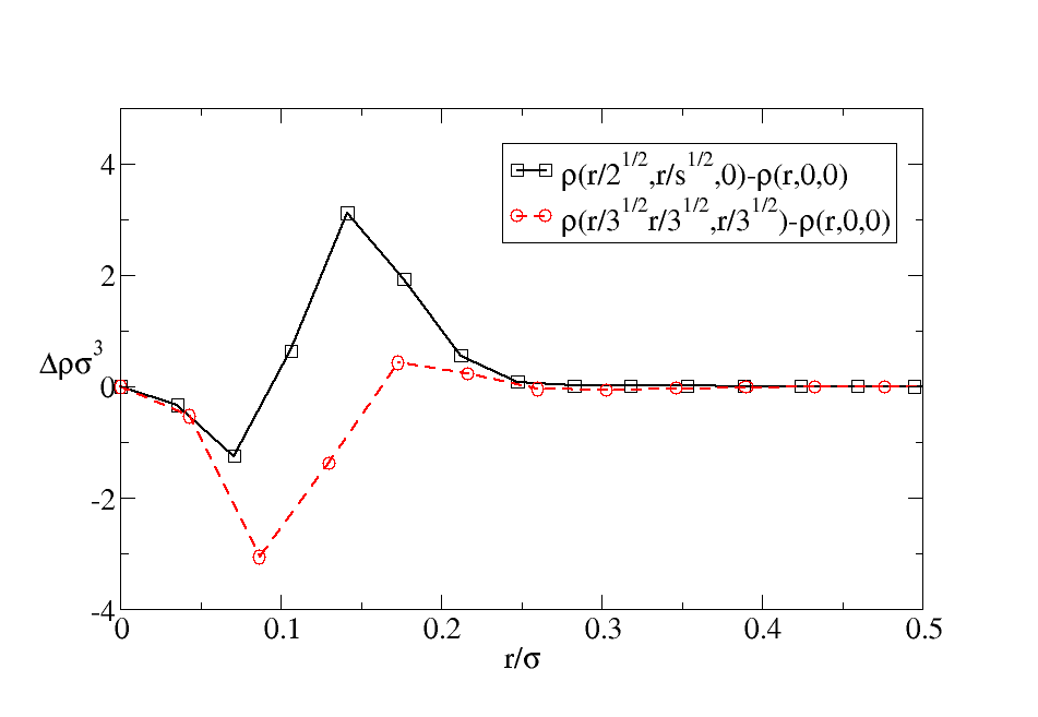
It has been seen that the use of Gaussian profiles produces results which are quantitatively very similar to the results of unconstrained minimization of the cDFT functional. Nevertheless, differences are expected due to the fact that the neighborhood of a lattice position in the solid is not spherically symmetric so that the Gaussian profiles, which force spherical symmetry of the contribution of each lattice site, can only be an approximation. In Fig. 9 we show the density profile for a LJ solid near the triple point ($k_{B}T=0.8$, $a=66\times 0.025\sigma=1.65\sigma$). The central region of the profile is well-fit by a Gaussian but away from the center, the distribution is much broader than a Gaussian. The difference is not due to contributions from the neighbors: the nearest neighbor distance is $a/\sqrt{2}$ and the best-fit Gaussian is $145e^{-95r^{2}}$ and a best fit normalized Gaussian has $\alpha=86$. Even taking the slightly broader latter function, the contribution at the half the nearest neighbor distance is $\left(\frac{86}{\pi}\right)^{1.5}e^{-86(0.5\times a/\sqrt{2})^{2}}\approx 3\times 10^{-11}$ which is much smaller than the excess in the tail of the density. Figure 10 shows the difference in density along lines running from a lattice position in the direction $(110)$ and $(111)$ relative to that along the $(100)$ direction and one sees that at intermediate distances, there is some asymmetry. This may be attributable to the fact that moving along the $(110)$ direction means towards a nearest neighbor and at this density, the nearest neighbor distance, $1.167\sigma$ is slightly more than the position of the minimum of the potential well, $1.12\sigma$, giving a small preference for adding density in that direction at the expense of the others.

The free energy difference between the FCC and HCP configurations is reported on Fig.11 as a function of the temperature. These DFT computations use the Gaussian profiles to parameterize the density field and have been performed for the WHDF potential with $r_{c}=1.2$ (colloid-like) and $r_{c}=2.0$ (simple fluid). For both potentials we get very similar free energies for the two configurations, about the order of magnitude of the expected interpolation error which is estimated to be $\Delta\beta\omega\sim 10^{-3}$ for the larger cutoff and an order of magnitude larger for the smaller cutoff. Such small differences are expected because these two structures only differ at the second neighbor. Wang et al. also state that simulations for the WHDF potential lead to very similar free energies for the FCC and HCP structures Wang et al. 2020. Our results indicate that the presented DFT model correctly reproduce this behavior and that using the FCC lattice gives a reasonable description of the solid free energies whether or not it is the most stable configuration.

References

- Evans (1979) R. Evans, “The nature of the liquid-vapour interface and other topics in the statistical mechanics of non-uniform, classical fluids,” Adv. Phys. 28, 143 (1979).
- Lutsko (2010) James F. Lutsko, “Recent developments in classical density functional theory,” Adv. Chem. Phys. 144, 1 (2010).
- Evans et al. (2019) Robert Evans, Maria C. Stewart, and Nigel B. Wilding, “A unified description of hydrophilic and superhydrophobic surfaces in terms of the wetting and drying transitions of liquids,” Proceedings of the National Academy of Sciences 116, 23901–23908 (2019), https://www.pnas.org/content/116/48/23901.full.pdf .
- Luukkonen et al. (2020) Sohvi Luukkonen, Maximilien Levesque, Luc Belloni, and Daniel Borgis, “Hydration free energies and solvation structures with molecular density functional theory in the hypernetted chain approximation,” The Journal of Chemical Physics 152, 064110 (2020), https://doi.org/10.1063/1.5142651 .
- Lutsko (2019) James F. Lutsko, “How crystals form: A theory of nucleation pathways,” Sci. Adv. 5, eaav7399 (2019).
- Rosenfeld (1989) Y. Rosenfeld, “Free-energy model for the inhomogeneous hard-sphere fluid mixture and density-functional theory of freezing,” Phys. Rev. Lett. 63, 980 (1989).
- Percus (1976) J. K. Percus, “Equilibrium state of a classical fluid of hard rods in an external field,” J. Stat. Phys. 15, 505–511 (1976).
- Percus (1981) J. K. Percus, “One-dimensional classical fluid with nearest-neighbor interaction in arbitrary external field,” J. Stat. Phys. 28, 67 (1981).
- Vanderlick et al. (1989) T. K. Vanderlick, H. T. Davis, and J. K. Percus, “The statistical mechanics of inhomogeneous hard rod mixtures,” J. Chem. Phys. 91, 7136 (1989).
- Roth (2010) Roland Roth, “Fundamental measure theory for hard-sphere mixtures: a review,” Journal of Physics: Condensed Matter 22, 063102 (2010).
- Oettel et al. (2010) M. Oettel, S. Görig, A. Härtel, H. Löwen, M. Radu, and T. Schilling, “Free energies, vacancy concentrations, and density distribution anisotropies in hard-sphere crystals: A combined density functional and simulation study,” Phys. Rev. E 82, 051404 (2010).
- Mortazavifar and Oettel (2016) Mostafa Mortazavifar and Martin Oettel, “A fundamental measure density functional for fluid and crystal phases of the asakura–oosawa model,” J. Phys.: Condens. Matter 28, 44018 (2016).
- Lutsko and Lam (2018) James F. Lutsko and Julien Lam, “Classical density functional theory, unconstrained crystallization, and polymorphic behavior,” Phys. Rev. E 98, 012604 (2018).
- (14) James F. Lutsko, “Explicitly stable fundamental measure theory models for classical density functional theory.” Http://arxiv.org/abs/2009.09390.
- Wang et al. (2020) Xipeng Wang, Simón Ramírez-Hinestrosa, Jure Dobnikar, and Daan Frenkel, “The lennard-jones potential: when (not) to use it,” Phys. Chem. Chem. Phys. 22, 10624–10633 (2020).
- Nelder and Mead (1965) J. A. Nelder and R. Mead, “A simplex method for function minimization,” The Computer Journal 7, 308–313 (1965).
- (17) M. Galassi et al, “Gnu scientific library,” http://www.gnu.org/software/gsl/, accessed: 2018-04-01.
- Guénolé et al. (2020) Julien Guénolé, Wolfram G. Nöhring, Aviral Vaid, Frédéric Houllé, Zhuocheng Xie, Aruna Prakash, and Erik Bitzek, “Assessment and optimization of the fast inertial relaxation engine (fire) for energy minimization in atomistic simulations and its implementation in lammps,” Computational Materials Science 175, 109584 (2020).
- Grosfils and Lutsko (2009) Patrick Grosfils and James F. Lutsko, “Dependence of the liquid-vapor surface tension on the range of interaction: A test of the law of corresponding states,” J. Chem. Phys. 130, 054703 (2009).
- Hansen and McDonald (1986) J.-P. Hansen and I.R. McDonald, Theory of Simple Liquids (Academic Press, San Diego, Ca, 1986).
- McRae et al. (1990) Robin McRae, John D. McCoy, and A. D. J. Haymet, “Density functional theory of vacancies,” Journal Chemical Physics 93, 4281 (1990).
- Singh and Das (2007) Sunil P. Singh and Shankar P. Das, “Perturbation theory for classical solids with vacancy defects,” Phys. Rev. B 75, 144113 (2007).
- Purohit et al. (2018) Apoorva Purohit, Andrew J. Schultz, Sabry G. Moustafa, Jeffrey R. Errington, and David A. Kofke, “Free energy and concentration of crystalline vacancies by molecular simulation,” Molecular Physics 116, 3027–3041 (2018).
Appendix A The FMT weights
In this Appendix, we give a somewhat simplified form for the analytic determination of the discrete FMT weights which is discussed in detail in the Supplementay material. For the local packing fraction, one needs to evaluate