Unification of variational multiscale analysis and Nitsche’s method,
and a resulting boundary layer fine-scale modelJournal: Computer Methods in Applied Mechanics and Engineering
Abstract
We show that in the variational multiscale framework, the weak enforcement of essential boundary conditions via Nitsche’s method corresponds directly to a particular choice of projection operator. The consistency, symmetry and penalty terms of Nitsche’s method all originate from the fine-scale closure dictated by the corresponding scale decomposition. As a result of this formalism, we are able to determine the exact fine-scale contributions in Nitsche-type formulations. In the context of the advection-diffusion equation, we develop a residual-based model that incorporates the non-vanishing fine scales at the Dirichlet boundaries. This results in an additional boundary term with a new model parameter. We then propose a parameter estimation strategy for all parameters involved that is also consistent for higher-order basis functions. We illustrate with numerical experiments that our new augmented model mitigates the overly diffusive behavior that the classical residual-based fine-scale model exhibits in boundary layers at boundaries with weakly enforced essential conditions.
Keywords:
Variational multiscale method , Nitsche’s method , weak boundary conditions , advection-diffusion equation , boundary layer accuracy , fine-scale Green’s function , higher-order basis functions1 Introduction
The variational multiscale (VMS) method was established in the 1990s by Hughes and coworkers as a universal framework for developing and classifying stabilized methods Hughes1995, Hughes1996, Hughes1998, Franca2006, Coley2018. It was hypothesized that the unresolved fine-scale nature of the solution of the partial differential equation is of key importance for the stability of finite-element schemes. The VMS methodology offers a means to ascertain the effect of the fine-scale solution onto the resolved finite element solution. As exact expressions for the fine scales are often not available, these fine-scale effects must be modeled. A particularly prevalent class of fine-scale models is that of the residual-based models Bazilevs2007. By assuming vanishing fine scales on element boundaries, the associated fine-scale problem can be solved on each element locally. The fine-scale solution is then approximated as the residual of the coarse-scale finite element solution, multiplied by the averaged Green’s function. It has been shown that the resulting stabilized formulation is closely related (and often equivalent) to classical stabilized methods Brezzi1997b, Hughes2004b. Typical examples include streamline-upwind Petrov-Galerkin (SUPG) Brooks1982, Brezzi1997b, Hughes2004b, tenEikelder2018, Galerkin least-squares (GLS) HUGHES1989173, Hughes2004b, tenEikelder2018, and pressure-stabilized Petrov-Galerkin (PSPG) methods Tezduyar1991. More recently, residual-based modeling of the fine scales has found its use as an effective turbulence model for finite element implementations of the Navier-Stokes equations Bazilevs2007, Codina2007, Masud2006, Chang2012, Wang2010, Gravemeier2011, Takizawa2014, tenEikelder2018ii. Since this turbulence model is mathematically inspired by the fine-scale equations, its parameters are clearly defined and it yields consistent formulations. Both these points are in contrast with typical eddy viscosity models, which are phenomenologically inspired and variationally inconsistent.
Another approach that has been shown to yield favorable results for fluid-mechanics applications is the use of weakly imposed Dirichlet boundary conditions Bazilevs2007weak_a, Bazilevs2007weak_b, bazilevs2010isogeometric. Typically, Nitsche’s method is the method of choice for weakly enforcing essential boundary conditions. While Nitsche’s method was initially proposed in relation to energy minimization functionals Nitsche1971, both its symmetric and nonsymmetric variants have since been studied extensively in fluid-mechanics applications Bazilevs2007weak_a, Bazilevs2007weak_b, bazilevs2010isogeometric, Burman2012. One of the main drivers for the significant recent interest in weakly enforced boundary conditions is their importance in immersed finite element methods. Notable references in the context of fluid mechanics include bazilevs2012isogeometric, xu2016tetrahedral, hsu2016direct, kamensky2015immersogeometric, wu2017optimizing, hsu2014fluid, hoang2019. For immersed finite element methods, the approximation space is no longer tailored to fit the domain boundary. The essential boundary conditions can thus not easily be satisfied strongly. Hence, there is a need for weakly enforcing the Dirichlet boundary condition in the weak formulation.
At first glance, the variational multiscale method and Nitsche’s method appear to be at conflict: the basis for a variational multiscale decomposition is a well-posed continuous weak formulation, but Nitsche’s method involves flexible spaces at Dirichlet boundaries and requires penalty terms that become unbounded in the continuous limit. Additionally, the fine-scale solution does, by design, not vanish on the Dirichlet boundary, which violates one of the key assumptions on which traditional residual-based fine-scale models are built. In previous work, we focused on discontinuous Galerkin methods, where the discontinuities between elements give rise to similar issues Stoter2017a, Stoter2017b, Stoter2019a. The goal of this article is to completely eliminate these issues for weak boundary imposition in Nitsche-type formulations.
The remainder of this article is structured as follows. In section 2, we derive a variational multiscale finite element formulation of the advection-diffusion equation and we show that Nitsche’s method arises from a particular choice of fine-scale closure. In section 3, we develop the fine-scale model that takes into account the non-vanishing fine scales at the Dirichlet boundary and provide estimates for the involved model parameters. The complete formulation is summarized in section 3.5. Next, in section 4, we show that the resulting bilinear form is coercive. In section 5, we verify the theory for a one-dimensional model problem, and in section 6 we computationally investigate the performance for a two-dimensional model problem that involves multiple boundary layers. In section 7, we present concluding remarks.
2 A variational multiscale derivation of the finite element formulation
The classical model problem for variational multiscale analysis is the steady advection-diffusion equation. Let denote the spatial domain with boundary . The governing equations in strong form read:
| in | (1a) | |||||||
| on | (1b) | |||||||
| on | (1c) | |||||||
| on | (1d) | |||||||
where the dependent variable maps into . The source function , the Dirichlet data and the Neumann (or Robin) data are exogenous functions that are assumed to be -integrable on their respective domains. The advective velocity is a given solenoidal vector field () and the diffusivity is strictly positive. The Dirichlet and Neumann (or Robin) boundaries and are complementary subsets of the boundary , i.e. , and the superscripts and indicate outflow () and inflow parts () respectively. On the boundary, the normal gradient is denoted . By convention, denotes the outward facing unit normal vector.
2.1 Variational multiscale weak formulation
To obtain the weak formulation we multiply by a test function and integrate by parts wherever suitable. Different from classical functional (and variational multiscale) analysis we keep the traces of our function spaces on the domain boundary variable. This requires the use of Lagrange multipliers for the enforcement of the Dirichlet boundary conditions. To ensure inf-sup stability of the resulting bilinear form, we substitute the known data on the inflow part of the Dirichlet boundary in the advective term. We then obtain the following weak formulation:
| (2a) | ||||
| (2b) | ||||
where denotes the -inner product on domain , and denotes the -inner product on a surface, which is to be interpreted in the sense of a duality pairing. In its current form, the suitable functional spaces may be identified as and . Equivalence of the strong and weak forms, eqs. 1 and 2, dictates that .
The variational multiscale approach splits the trial solution and test function spaces into coarse and fine scales. The coarse scales live on the finite element grid, whereas the fine scales are determined via a model equation. This decomposition may be written as:
| (3) |
where is the space spanned by the finite-dimensional discretization and the fine-scale space is an infinite-dimensional complement in . The components of the solutions and test functions decouple as
| (4a) | ||||
| (4b) | ||||
with coarse scales and fine scales . The direct sum decomposition in eq. 3 is associated with a projection operator:
| (5a) | ||||
| (5b) | ||||
where is the projector and is the identity operator. Formally, this projector is incorporated in the weak formulation through the definition of the fine-scale space . It follows from eq. 5b that . Then, the direct sum decomposition of eq. 3 ensures the unique decomposition that satisfies eqs. 4 and 5. Using this multiscale split we arrive at the following alternative – equivalent – weak statement:
| (6a) | ||||
| (6b) | ||||
| (6c) | ||||
Equation (6a) is the ‘coarse-scale problem’, and can be interpreted as a relation for for a given and . The Lagrange multiplier is taken care of by substituting the known value in the continuous case, viz. . Similarly, the ‘fine-scale problem’ of eq. 6b can be conceived as a relation for the fine-scale component . This space, however, is infinite-dimensional and is thus not amenable to discrete implementation. Hence, in eq. 6a a closure model will be substituted in place of the fine-scale solution.
2.2 Nitsche’s method as a partial fine-scale closure
Next, we show that a particular fine-scale closure condition leads to Nitsche’s classical formulation. Our goal is to illustrate that Nitsche’s method and the accompanying penalty terms are not in conflict with the VMS theory, but rather can be interpreted naturally in the VMS framework as a particular choice of fine-scale closure. Consider the following projection operator, which we will refer to as the Nitsche projector:
| (7) |
By taking the Gâteaux derivative and subsequently replacing by , we obtain the following associated optimality condition for the fine scales:
| (8) |
Note that eqs. 7 and 8 involve integrals of the normal derivative of functions in on the boundary of . In order for these integrals to be well-defined for all , we require a redefinition of . If we set with , then:
| (9) |
defines on the boundary for all . Given that we are considering data of the form , the true solution will automatically be an element of this new space.
Typically, in the variational multiscale framework, one would attempt to invert the fine-scale problem of eq. 6b while satisfying the requirement posed by eq. 8. However, the particular structures of the coarse-scale problem and the Nitsche projector allow for a more direct inversion of (part of) the fine scales in the coarse-scale equation Stoter2017b, Stoter2019a. First, we recognize that the fine-scale terms in eq. 8 on the Dirichlet boundary may be written in terms of the coarse-scale solution through the definition . Then, since eq. 8 holds for all , we may choose and add the obtained equality to the coarse-scale problem of eq. 6a. By following this procedure we are left with Nitsche’s formulation of the advection-diffusion problem:
| (10) | ||||
where only one fine-scale term remains. We emphasize that both the symmetric term of Nitsche’s method as well as its penalty term originate from the fine-scale inversion per eq. 8.
Remark 1: If we write the remaining fine-scale term as , then we observe that the appropriate fine-scale model (read: stabilization technique) in conjunction with Nitsche’s method involves the SUPG operator . Typically, in variational multiscale stabilized methods, the adjoint differential operator is proposed. However, since the diffusive part of the fine-scale terms has already been incorporated via the introduction of the Nitsche terms, the diffusive operator no longer occurs in the fine-scale term.
2.3 Analysis of the Nitsche projector
The projector defines the scale decomposition of eq. 3 via eq. 5. This means that it impacts the appropriate modeling choices in the development of the fine-scale model. Before continuing the fine-scale modeling, we thus first dedicate a short study on the Nitsche projector. The ensuing analysis will heavily rely on the work by Hughes and Sangalli in Hughes2007, who performed the same analysis using the and projectors.
A projector may be defined by a finite number of functional constraints; as many as the dimension of :
| (11) |
The functionals for the Nitsche projector may be inferred from the weak statement of eq. 8. By performing integration by parts on its first term while interpreting the resulting integral in the sense of distributions, the functional constraints follow from substituting the various candidates for . For a one-dimensional domain with a set of nodes and element domains and a typical nodal finite element construction of with polynomial order , we find:
| (12a) | ||||||
| (12b) | ||||||
| (12c) | ||||||
| (12d) | ||||||
The first requirement dictates nodal exactness of the finite element formulation, and together with the second requirement these define the projector Hughes2007. The last two originate from the extra degrees of freedom on the Dirichlet boundary.
Remark 2: The central role of the projector can be useful for the interpretation of the obtained finite element solution. For instance, for the current example of Nitsche’s method, a better approximation of the true diffusive flux on the Dirichlet boundary could be obtained by rewriting eqs. 12c and 12d:
| (13a) | ||||||
| (13b) | ||||||
The same expressions were also proposed in Bazilevs2007weak_a by Bazilevs et al., although motivated based on discrete conservation laws.
Remark 3: In Harari2018, Harari and Albocher perform a spectral analysis of Nitsche’s formulation. Their work shows that its spectrum consists of i) traditional modes that are independent of the Nitsche parameter and which vanish on Dirichlet boundaries, and ii) modes that depend on the Nitsche parameter and are locally supported in a layer along the Dirichlet boundaries. In eq. 12, we observe a similar split in the (functional) constraints imposed by the Nitsche projector.
3 A residual-based multiscale model with non-vanishing fine-scale boundary values
For our finite element scheme to yield solutions close to , the weighted integral of in formulation (10) needs to be accurately modeled. The model for the remaining fine-scale quantity originates from the inversion of the fine-scale problem of eq. 6b.
3.1 Inversion of the fine-scale problem
Consider the following general form of the fine-scale problem:
| (14) |
By performing the appropriate integration by parts steps we obtain the following integral relation, to be interpreted in the sense of distributions:
| (15) |
where we denote our spatial variable , for ease of notation later on. The operator is the adjoint of the differential operator , the coarse-scale residual is denoted , and is a bilinear form that represents the boundary terms.
Then, we hypothesize that one can find a function such that acts on any function in in the following way:
| (16) |
where we call this particular function the fine-scale Green’s function . The denotes the Dirac delta distribution at , and the functionals refer to the functional constraints from eq. 11. The sum provides a relaxation such that may be found in the constrained space . From eq. 15 we obtain:
| (17) |
where the summation vanishes due to eq. 11, and the term incorporates the fine-scale boundary conditions. This relation determines from a given .
3.2 Adoption of the fine-scale Green’s function
The fine-scale Green’s function in eqs. 16 and 17 corresponds to the Nitsche projector. However, most literature on the variational multiscale method focuses on a scale decomposition by means of the projector. To maintain the connection with existing fine-scale models, we reintroduce the fine-scale Green’s function as follows:
| (18) |
The newly added subscripts indicate the projector with which the fine-scale Green’s function is associated. The similarity between the projector and the Nitsche projector can be expressed in terms of their imposed functional constraints, from eq. 11. The set of functions corresponding to the projector is a subset of those of . If we order the set such that coinciding occurrences come first, then we may write for the fine-scale Green’s function:
| (19) |
which, after substitution in eq. 16, gives a result for :
| (20) |
Substitution of eq. 18 into eq. 17 while using gives:
| (21) |
where the last equality results from performing the integration by parts steps of eq. 15 in reverse.
By using eq. 20 in the last term of eq. 21, it follows from eq. 11 that this term vanishes when . The expression for becomes:
| (22) |
Remark 4: The inversion posed by eq. 22 is no longer unique; it is satisfied for solutions , but also for solutions . However, the partial fine-scale closure discussed in section 2.2 is not satisfied by . The formulation obtained after substitution of eq. 22 into Nitsche’s coarse-scale formulation of eq. 10 will hence be uniquely satisfied by .
Recall that the term enforces the fine-scale boundary conditions. The original residual-based model assumes that the fine-scale solution vanishes on element boundaries Bazilevs2007. Since we aim not to make this assumption, this will be the key term that we retain to obtain a more suitable fine-scale model. In eq. 22, this term simplifies since is zero on the boundary. We then restrict our analysis to partial differential equations for which we may write:
| (23) |
with being some differential operator. This includes the advection-diffusion operator, for which is:
| (24) |
The only term in the coarse-scale formulation of eq. 10 in which appears is the advective term. We thus finally obtain the fine-scale contribution to the coarse-scale equation as:
| (25) | ||||
The unknown data on the Neumann boundary, together with the double integration and the limited availability of Green’s functions, make the closure relation of eq. 25, albeit exact, unsuitable for computational use. Simplifications via approximations need to be introduced. The strategy that we will employ repeatedly in this article is to reformulate such that exactness is maintained in the case of constant physical parameters on a one-dimensional domain, while ease of implementation is established in the general case.
3.3 The classical one-dimensional case
In the one-dimensional case, the nodal exactness induced by the projector results in an element-local fine-scale Green’s function Hughes2007. The double integrals in eq. 25 can thus be split in contributions of individual elements. The newly added term only affects elements that lie adjacent to the Dirichlet boundary, where the precise value of the fine-scale solution is known as . On Neumann boundaries the new term vanishes due to eq. 12a. Let us consider the contribution of one element that shares a node with the Dirichlet boundary:
| (26) | ||||
To simplify, we use the polynomial representation of the test function and the residual . When is constructed with -order nodal elements and the source function is at most polynomial order , then:
| (27) |
We also have the following properties of the fine-scale Green’s function :
| (28a) | ||||||
| (28b) | ||||||
Property (28a) is shown in Hughes2007, and we prove (28b) in A.1. Substituting eq. 27 into eq. 26 while using eq. 28 yields:
| (29) | ||||
We assume to be constant in , and we extract and all other constants from the double integration. We then integrate the two right hand side terms over and respectively, and we divide them by and :
| (30) | ||||
where we can identify the following model parameters:
| (31a) | ||||||
| (31b) | ||||||
The multiplication and division by in eq. 30 ( being the element size) ensures that the parameters in eq. 31 remain dimensionally consistent with varying polynomial order.
3.4 Fine-scale closure generalization
Up until now, all derivations have been exact. To make use of the integral expressions in eq. 30 on multi-dimensional domains, we approximate them by the following inner products:
| (32a) | ||||||
| (32b) | ||||||
As eq. 32b indicates, we only make use of the newly proposed term at the outflow Dirichlet boundary . This is where the boundary layers occur, and where the weak enforcement of the Dirichlet conditions results in impactful fine-scale boundary values.
All the approximations involved in the final finite element formulation may be traced back to these two equations. Essentially, they shift the modeling effort onto the effective stabilization parameters and . We propose to design and such that these are approximations of and that take into account the change of (bi)linear forms, while being suitable for multi-dimensional computations for arbitrary order polynomial basis functions.
3.4.1 Estimation of operator impact
In the one-dimensional case, the bilinear forms of the left-hand and right-hand sides of eq. 32 may be written as:
| (33a) | ||||||
| (33b) | ||||||
| (33c) | ||||||
| (33d) | ||||||
The impact of these different bilinear forms may be quantified by considering their norms:
| (34) |
where we have chosen to define the norm of the bilinear forms with respect to the -seminorm of its arguments, as this seminorm is one of the terms in the optimality condition induced by the Nitsche projector according to eq. 7.
We choose and such that the impact of these bilinear forms equal: and . If we assume constant parameters in , and the advective dominant case such that may be approximated by , then we obtain:
| (35a) | ||||||
| (35b) | ||||||
The inverse inequalities in these expressions are computable by hand harari1992c. For linear, quadratic and cubic coarse-scale basis function, the relations between the parameters and , and and become:
| (36) |
3.4.2 -parameter approximation for
In literature, we find that the -parameter that is used with higher-order basis functions is often the same as that for (i.e., obtained from the element local Green’s function), sometimes with a -dependent mesh size scaling. In this section, we propose an approximation of for linear, quadratic and cubic elements based on the actual fine-scale Green’s functions. These are devised such that they limit to the exact expressions in the advection () or diffusion () dominated cases. Using the definition of from eq. 31a, together with the fine-scale Green’s functions from A, the following exact expressions for may be computed for and respectively Brooks1982, Hughes1995, Hughes2007:
| (37a) | ||||||
| (37b) | ||||||
| (37c) | ||||||
where is the element Péclet number and is the upwind function. From these equations we obtain the following advective and diffusive limits:
| (38a) | ||||||
| (38b) | ||||||
| (38c) | ||||||
The following approximation strategy for is used frequently in stabilized methods Hughes1986, Tezduyar1991, Shakib1991, Tezduyar2000, Bazilevs2007:
| (39) |
To determine the effectiveness of the scaling for the various polynomial orders, we substitute eq. 38 into (39). In all cases, we can rewrite the expression to obtain the effective approximate upwind function. For example, for linear elements:
| (40) |
Figure 1a illustrates how the approximate upwind functions relates to the exact upwind functions of eq. 37. The figure shows that the approximation of according to eq. 39 has the correct asymptotic limits, and converges to these limits at the correct rates. We observe that this holds for each polynomial order.
3.4.3 -parameter approximation for
In a similar sense, we wish to construct an approximate , based on generic (spatial dimension independent) parameters, that share the asymptotic scaling behavior of the exact one-dimensional expression. The exact expressions of may be computed from eq. 31b as:
| (41a) | ||||||
| (41b) | ||||||
| (41c) | ||||||
for and respectively. is a boundary type element Péclet number. Since we only make use of on the outflow boundary (), we exclusively consider in the following. The advective and diffusive limits of these expressions are:
| (42a) | ||||||
| (42b) | ||||||
| (42c) | ||||||
Since these limits do not depend on nor on , the approximation strategy of eq. 39 is not viable. Instead, we deduce the following scaling of based on its definition from eq. 31b:
| (43) |
where represents the scaling induced by as defined in eq. 24, and is a modified -like quantity that takes into account the difference in domain of integration between and in eq. 31. scales linearly with and inversely with length, such that we may choose . By adopting a similar approximation for as eq. 39, we obtain:
| (44) |
takes into account the shape effect of the element as the measure of the relevant boundary versus the measure of the element interior:
| (45) |
where the multiplication with ensures a mesh size independent scaling, and should be the representative element size that is used in the approximation of through and . In this article we use the longest element edge. In the one-dimensional case and , such that .
The coefficients and are introduced to capture the difference in scaling between and . They can be determined from eq. 44 by ensuring the correct limiting behavior of in the one-dimensional case. For example, for linear elements, substituting the limits of eq. 38a results in:
| (46) |
By ensuring that eq. 46 has the same asymptotic limits as eq. 41 and also has the same convergence rate towards zero, we obtain and . The same strategy results in and for and and for . Figure 1b shows the approximate and exact boundary functions and confirms that the approximation of displays the correct asymptotic scaling behavior for all polynomial orders.
3.5 Complete finite element formulation
With all the modeling terms included, the finite element formulation becomes:
| (47) | ||||
where the advection and diffusion parts of the bilinear form are:
| (48a) | ||||
| (48b) | ||||
and where the two variational multiscale components are:
| (49a) | ||||
| (49b) | ||||
with the sum of open element domains.
Expressions for the parameters and are collected in Table 1. These expressions take into account all the considerations discussed in sections 3.4.2, 3.4.3 and 3.4.1. As the table shows, we have formulated all model parameters such that they depend exclusively on and , i.e., those relating to linear elements. The exact approach for computing these limiting values remains flexible. For example, one could incorporate the Jacobian of the element mapping Bazilevs2007, Bazilevs2007weak_b, use element local length-scales and Péclet numbers Tezduyar2000, or use the analytical expressions of eq. 38a and the element diameter.
| : | ||||
|---|---|---|---|---|
| : | ||||
| Element: | ||||
| (eq. 45): | 1 | |||
4 Analysis of existence and uniqueness
As touched upon in Remark 4 in section 3.2, the uniqueness of the fine-scale inversion is not a trivial issue. Additionally, the required simplification and modeling steps discussed in section 3.4 may raise further questions regarding the existence of the approximate coarse-scale solution. In a finite-dimensional functional setting, existence and uniqueness follow directly from the coercivity of the bilinear form, which we analyze in this section.
In the analysis, we assume that and are constant in and that the grid is (quasi) uniform, such that also , and can be chosen as global constants. The derivations can trivially be modified for non-uniform grids or non-constant and and element-wise parameters , and . We further assume that the parameter satisfies:
| (50) |
The first inequality is satisfied due to the harmonic mean structure of , where the ’s follow directly from table 1 as 1, and for linear, quadratic and cubic basis functions respectively. On a one-dimensional mesh, this means that , and . In this one-dimensional case, the inverse estimate in eq. 50 may be explicitly computed, resulting in maxima of , and for polynomial orders of 1, 2 and 3. The condition of eq. 50 is thus satisfied. We expect similar results in multiple spatial dimensions for meshes with reasonable quality.
Finally, we require that satisfies:
| (51) |
with:
| (52a) | ||||
| (52b) | ||||
We carry out the coercivity proof for the different components of the bilinear forms separately, and then look at the formulation as a whole. We start with determining a relation between the model parameters and .
Lemma 4.1.
For , or , the expressions from table 1 are such that is bounded by according to:
| (53) |
Proof.
We write the and expressions from table 1 in the following general form:
| (54) | ||||
| (55) |
Dividing by and squaring gives:
| (56) |
After multiplying both sides by and using , we obtain:
| (57) |
The fraction may be bound from above as:
| (58) |
Equation 53 follows from the maximum of the three cases. ∎
Lemma 4.2.
The bilinear form in eq. 48a satisfies the following coercivity result:
| (59) |
where the norms are norms on the indicated domains.
Proof.
Lemma 4.3.
Proof.
Lemma 4.4.
Proof.
Direct substitution of results in:
| (66) |
With Young’s inequality we bound the second term from below:
| (67) |
Using the assumed bound of from eq. 50 completes the proof. ∎
Lemma 4.5.
The boundary variational multiscale term in eq. 49b satisfies the following coercivity result:
| (68) |
where the norms are norms on the indicated domains.
Proof.
After substitution of , we obtain:
| (69) | ||||
| (70) |
The first inequality follows from Young’s inequality with parameter , and the second inequality as well as the parameter originate from the inverse estimate of eq. 52b. Choosing the parameter and using the result of Lemma 4.1 to relate and completes the poof. ∎
Theorem 4.1.
The combined bilinear form of eq. 47 satisfies the following coercivity result:
| (71) |
where the norms are norms on the indicated domains.
Proof.
Remark 5: Note that both Nitsche’s method (Lemma 4.3) and the VMS method (Lemma 4.4) rely on the first term in eq. 63 for their stability. As a result, the combined use of VMS and weakly enforced boundary conditions requires a larger / ratio compared to the typical choice of for the standard Nitsche’s method Embar2010.
5 Numerical verification for a one-dimensional model problem
We present a number of numerical experiments to verify the derivation from sections 3.1, 3.2 and 3.3, and to investigate the accuracy improvement that may be achieved by using the new residual-based fine-scale model of sections 3.4 and 3.5.
5.1 Linear basis functions
Figure 2 shows the result for a simulation with , and on the domain , discretized with three linear elements. The solid green line shows the exact solution . With the current discretization, the boundary layer falls completely within a single element. We obtain the exact coarse-scale solution, indicated with the black line, by projecting the exact solution onto the finite element mesh with the Nitsche projector from Section 2.2. The blue dotted line is obtained by only using the classical VMS term, equivalent to , whereas the red dashed solution incorporates the exact augmented VMS model from eq. 30 with the exact parameter definitions from eq. 31. Finally, the line with the circular markers shows the result when the generalized model of sections 3.4 and 3.5.
It is a celebrated fact that for this model problem the VMS method with strongly enforced boundary conditions results in nodally exact solutions Hughes1998. The results of Figure 2a show that this property is lost when the boundary conditions are enforced weakly, and that the under-resolved boundary layer affects the approximation on a large part of the domain. Figure 2b shows that the magnitude of the fine-scale solution on the outflow boundary of the domain is considerable. Hence, the assumption of vanishing fine scales, which is critical in the derivation of the classical VMS model, is severely violated. In contrast, the augmented VMS model is exactly the Nitsche projection of the exact solution. As a result, the nodal exactness of the computational solution is retrieved and the adverse effect of the boundary layer is constrained to a single element. Due to the relative simplicity of this problem, solution obtained with the generalized model is only affected by the estimation of the model parameters. As it is nearly identical to the exact coarse-scale solution we conclude that, at least for this simple case, the estimation strategy is effective.
Remark 6: It is well known that for the current case the classical VMS term simplifies to a (consistent) diffusion term. Interestingly, in a similar sense the augmented term in the VMS formulation simplifies to a reduced diffusion in the symmetric part of Nitsche’s formulation. In this context, the solution obtained by using the classical VMS model may be interpreted as excessively diffusive in the boundary layer, which is (consistently) counteracted by the augmented VMS term.
5.2 Higher-order basis functions
We use the same problem formulation but discretize with three higher-order elements. With quadratic basis functions and we obtain the solutions from Figures 3a and 3b, and with cubic basis function and we obtain the solutions from Figures 3c and 3d. We can largely draw the same conclusions as for the linear basis functions: the fine-scale solution deviates significantly from zero at the outflow boundary. As a result, the solution quality of the classical VMS model is spoiled. By using the augmented VMS model we obtain the Nitsche projection of the exact solution. This gives a nodally exact solution, where the adverse effect of the boundary layer is contained within the boundary element. These points are all compliant with the theory of section 2.2.
Additionally, we observe that the solution for the approximate augmented VMS model is very close to the exact coarse-scale solution. For the linear basis functions we concluded that the estimations of the model parameters are effective. We can now also conclude that the approximation of the differential operator described section 3.4.1 is effective, at least for this one-dimensional case.
6 Numerical experiments for a two-dimensional model problem
Next, we present numerical experiments for a two-dimensional domain. All the model approximations become important, and their effectiveness can be assessed.
6.1 Linear basis functions, high and low advective dominance
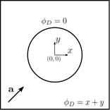
We consider a model problem of a unit square with a circular hole of radius 0.24 in the center. Dirichlet conditions are enforced on all boundaries; around the circular cut-out, and around the square. The advective field acts across the diagonal with a magnitude of , the diffusivity is or , and we use . Figure 4a schematically illustrates the model problem, and Figure 4b shows the solution for obtained with a highly refined mesh. The solution features multiple boundary layers at various orientations.
The performance of the models can most clearly be assessed by investigating the resulting fine-scale solutions. These are shown in Figures 5 and 6 for and respectively. In Figures 5a and 6a classical VMS stabilization is used (i.e. ), and Figures 5b and 6b show the results for the augmented model. Additionally, we project the overrefined solution onto the coarse-scale function space using the Nitsche projector, and show the resulting fine-scale solution in Figures 5c and 6c. This represents the ‘exact’ fine-scale solution.


The observations made for the one-dimensional case almost directly transfer to this two-dimensional problem. The Nitsche projector aims to constrain the impact of the high gradients to the boundary layer elements, without spoiling the results further into the domain. This is illustrated by large fine-scale solutions in only a single row of elements adjacent to the outflow boundary. When the classical VMS model is used, we observe a significant thickening of the range of nonzero fine scales; interpretable as excessive diffusion in the coarse-scale solution. When we add the additional modeling term this thickening is decreased, which leads to nearly the same solution quality as that obtained with the Nitsche projection. We observe these effects irrespective of the Péclet number.
To further illustrate the significance of the change, we show all three solutions on a cut-plane in Figure 7. Note, in particular, the similarity of Figure 7b and the corresponding figure for the one-dimensional case (Figure 2b). The fine-scale solution corresponding to a completely non-stabilized computation is also plotted to put the overall improvement of the solution quality into context.
Convergence in the or (semi)norms are not indicative of solution quality for the current case; projections of shocks lead to highly oscillatory solutions such that the non-stabilized solution often achieves the lowest error, and neither the classical nor the augmented VMS model aims to achieve optimality in the seminorm as the boundary conditions are not enforced strongly. Rather, the use of weakly enforced boundary conditions implies the optimality condition of eq. 8, satisfied by solutions that minimize eq. 7. The error of interest is thus the one with respect to the ‘optimal’ solution; the exact coarse-scale solution obtained with the Nitsche projector. This error indicates the performance of the fine-scale model. This error is plotted for different mesh densities in Figures 8a and 8b. Figures 5, 6 and 7 correspond to the third data point in these convergence graphs. Both graphs show a considerable reduction in error when the augmented VMS model is used, which persists throughout mesh refinement. We observe that the () error reduction from classical to augmented VMS is often of the same magnitude, if not larger, than from non-stabilized to classical VMS.
Remark 7: Analogous to the one-dimensional case, the augmented VMS term decreases the diffusivity in the symmetry part of the Nitsche formulation. Different from the one-dimensional case, this becomes vector-valued and the formulation becomes a streamline directed modified diffusion on the boundary. One could interpret this as a boundary equivalent of the streamline diffusion that the classical VMS terms revert to for the same case.
6.2 Higher-order basis functions
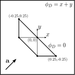
Next, we change the geometry to a square with a polygonal exclusion, as depicted in Figure 9. An exact geometry representation can be achieved, which, for these higher-order basis functions, is important for accurately computing the boundary integrals for the Nitsche projection . We focus on the advection dominated case of and , and we use .
Figures 10a, 10b and 10c show the fine-scale solutions for quadratic basis functions obtained with the classical VMS model, the augmented VMS model and the Nitsche projector respectively. We observe that the classical VMS model with the parameter estimation developed in sections 3.4.1 and 3.4.2 already performs remarkably well. The boundary layers are almost exclusively contained in a single row of elements.
When we add the augmented term in the VMS model, the obtained error field qualitatively more closely resembles the true fine-scale solution shown in Figure 10c. We do, however, also observe some small oscillations. This is consistent with the decreased diffusion interpretation proposed in Remarks 6 and 7. A more detailed analysis of the resulting error confirms that the solution obtained with the augmented VMS model more closely resembles the true coarse-scale solution defined by the Nitsche projector. This is shown in Figure 11a, where the resulting fine-scale solution is plotted along a cut-plane, as well as in Figure 11b, which plots the -error with respect to the true coarse-scale solution for various mesh densities.


Finally, if we use cubic basis functions, we obtain the results from Figures 12 and 13. Similar conclusions may be drawn as for the case of quadratic basis functions: the classical model with the parameters from Table 1 leads to a coarse-scale solution where the error is contained in the first row of elements. Adding the augmented term results in a solution that exhibits small oscillations, but nonetheless bears closer resemblance to the true coarse-scale solution, as measured qualitatively in Figure 13a and quantitatively in Figure 13b.
It should also be noted that the Dirichlet boundary conditions are more closely satisfied with these cubic basis functions, as shown in Figure 13a. This is, at least in part, due to the larger penalty parameter . The near-strong enforcement of the Dirichlet condition leaves a small fine-scale boundary value. The new term in the augmented model becomes almost inoperative, and the classical VMS model suffices. Indeed, the difference between the augmented and classical models is not as pronounced as it was in earlier simulations. These results convey that the augmented model provides fine-scale corrections in the pre-asymptotic regime, and vanishes (asymptotically) when such fine-scale corrections cease to be relevant.


7 Conclusion
In this article, we unify the theories of variational multiscale analysis and weakly enforced boundary conditions into one consistent framework. Individually, these elemental numerical methods have shown great value in the context of fluid mechanics. With their merger, we are in a position to develop a fine-scale model that is appropriate for use in combination with Nitsche’s method.
When the Dirichlet boundary conditions are enforced weakly, the standard projector is no longer applicable for the scale decomposition around which the variational multiscale method revolves. Instead, we propose a new projector, which we call the Nitsche projector. We show that adoption of this projector in the multiscale formulation naturally leads to Nitsche’s formulation. That is, both the penalty term and the symmetry term in Nitsche’s formulation automatically fall into place as part of the variational multiscale scale decomposition.
The model for the remaining fine-scale terms is based on the inversion of the fine-scale problem, which, in turn, is formally posed in the kernel space of the projector. We show that the functional constraints that define the projector are a subset of those corresponding to the Nitsche projector, such that we can largely base the inversion of the fine-scale problem on existing theory. An important difference in the context of weakly enforced boundary conditions is that the assumption of vanishing fine scales on element boundaries is no longer applicable for elements adjacent to the Dirichlet boundary. As a result, the fine-scale model that we obtain is the classical VMS model plus an additional boundary term. This ‘augmented’ term takes into account the non-vanishing fine scales on the Dirichlet boundary. It may be interpreted as a consistent streamline diffusion in the symmetry term of Nitsche’s formulation.
Additionally, we develop approximations for the modeling terms and based on the fine-scale Green’s functions. These expressions and approximation strategies are also suitable for discretization with higher-order elements.
With this new model, and these new parameter definitions, we retrieve nodally exact solutions on one-dimensional meshes for all polynomial orders. This is an important property of the classical VMS model, which is lost when the boundary conditions are enforced weakly. On two-dimensional domains, we observe that the augmented model more closely resembles the actual coarse-scale solution defined by the Nitsche projector, as measured in an sense. This holds for all polynomial orders. For quadratic and cubic basis functions, the model without the augmented term already performs very well with the newly developed approximations. The error due to the boundary layer is contained in a single row of elements. For linear basis functions, however, the classical VMS model leads to a too thick boundary layer. This is almost completely mitigated when the augmented model is added to the formulation.
Acknowledgments. D. Schillinger gratefully acknowledges support from the National Science Foundation via the NSF CAREER Award No. 1651577 and from the German Research Foundation (Deutsche Forschungsgemeinschaft DFG) via the Emmy Noether Award SCH 1249/2-1. M.F.P. ten Eikelder and I. Akkerman are grateful for the support of Delft University of Technology.
Appendix A Fine-scale Green’s functions and ’s vanishing moments
In this appendix we draw conclusions on the expression for the fine-scale Green’s functions corresponding to and polynomial basis functions. Recall the definition of :
| (74) |
where we now add the superscript to the fine-scale Green’s function to denotes the polynomial order of the coarse-scale basis functions on which projects.
The fine-scale Green’s function associated to the -projector has been studied extensively in Hughes2007. The authors prove the element local nature of in the one-dimensional case. They also show that in a single element, the fine-scale Green’s function can then be obtained from the element local classical Green’s function:
| (75) | ||||
Refer to Stoter2017a or Hughes2004b for the expression for . The resulting functions for and are plotted in Figure 14. For this particular case, the fine-scale Green’s function for is exactly the element local classical Green’s function .


The derivation in section 3.3 requires vanishing ‘moments’ of the fine-scale Green’s function, as stated in eq. 28b. We prove that this holds for in the following theorem.
Theorem A.1.
Define a -like parameter that depends on coarse-scale polynomial order and a th moment:
| (76) |
then from the definition of in eq. 75 it follows that:
| (77) |
Proof.
The equality for follows directly from the definition of . For we substitute the definition of the fine-scale Green’s function from eq. 75. After carrying out the integration in eq. 75, the first vector becomes independent of the -variable, and the last vector independent of the -variable. The center matrix is filled with constants. This means that the differential operator and integration from eq. 76 act on different vectors and they can thus be separated. After re-ordering of derivatives and integrals we obtain:
| (78) | ||||
For ease of notation we denote the involved vectors and matrix , and . By recognizing that is the th row of C we can write , where is a vector of zeros with a 1 at the th row. Substitution into the matrix-vector multiplication yields:
| (79) |
Note that this only holds for , since C has rows. ∎
References
- [1] T.J.R. Hughes. Multiscale phenomena: Green’s functions, the Dirichlet–to–Neumann formulation, subgrid scale models, bubbles and the origins of stabilized methods. Computer Methods in Applied Mechanics and Engineering, 127(1-4):387–401, 1995.
- [2] T.J.R. Hughes and J.R. Stewart. A space–time formulation for multiscale phenomena. Journal of Computational and Applied Mathematics, 74(1-2):217–229, 1996.
- [3] T.J.R. Hughes, G.R. Feijóo, L. Mazzei, and J.-B. Quincy. The variational multiscale method – a paradigm for computational mechanics. Computer Methods in Applied Mechanics and Engineering, 166(1-2):3–24, 1998.
- [4] L.P. Franca, G. Hauke, and A. Masud. Revisiting stabilized finite element methods for the advective–diffusive equation. Computer Methods in Applied Mechanics and Engineering, 195(13-16):1560–1572, 2006.
- [5] C. Coley and J.A. Evans. Variational multiscale modeling with discontinuous subscales: analysis and application to scalar transport. Meccanica, 53(6):1241–1269, 2018.
- [6] Y. Bazilevs, V.M. Calo, J.A. Cottrell, T.J.R. Hughes, A. Reali, and G. Scovazzi. Variational multiscale residual-based turbulence modeling for large eddy simulation of incompressible flows. Computer Methods in Applied Mechanics and Engineering, 197(1-4):173–201, 2007.
- [7] F. Brezzi, L.P. Franca, T.J.R. Hughes, and A. Russo. . Computer Methods in Applied Mechanics and Engineering, 145(3-4):329–339, 1997.
- [8] T.J.R. Hughes, G. Scovazzi, and L.P. Franca. Multiscale and stabilized methods. In E. Stein, R. De Borst, and T.J.R. Hughes, editors, Encyclopedia of computational mechanics, chapter 4. John Wiley & Sons, Ltd, 2004.
- [9] A.N. Brooks and T.J.R. Hughes. Streamline upwind/Petrov–Galerkin formulations for convection dominated flows with particular emphasis on the incompressible Navier–Stokes equations. Computer Methods in Applied Mechanics and Engineering, 32(1-3):199–259, 1982.
- [10] M.F.P. ten Eikelder and I. Akkerman. Correct energy evolution of stabilized formulations: The relation between VMS, SUPG and GLS via dynamic orthogonal small-scales and isogeometric analysis. I: The convective–diffusive context. Computer Methods in Applied Mechanics and Engineering, 331:259–280, 2018.
- [11] T.J.R. Hughes, L.P. Franca, and G.M. Hulbert. A new finite element formulation for computational fluid dynamics: VIII. The Galerkin/least–squares method for advective–diffusive equations. Computer Methods in Applied Mechanics and Engineering, 73(2):173–189, 1989.
- [12] T.E. Tezduyar. Stabilized finite element formulations for incompressible flow computations. Advances in Applied Mechanics, 28(C):1–44, 1991.
- [13] R. Codina, J. Principe, O. Guasch, and S. Badia. Time dependent subscales in the stabilized finite element approximation of incompressible flow problems. Computer Methods in Applied Mechanics and Engineering, 196(21):2413–2430, 2007.
- [14] A. Masud and R.A. Khurram. A multiscale finite element method for the incompressible Navier–Stokes equations. Computer Methods in Applied Mechanics and Engineering, 195(13-16):1750–1777, 2006.
- [15] K. Chang, T.J.R. Hughes, and V.M. Calo. Isogeometric variational multiscale large-eddy simulation of fully-developed turbulent flow over a wavy wall. Computers & Fluids, 68:94–104, 2012.
- [16] Z. Wang and A.A. Oberai. A mixed large eddy simulation model based on the residual-based variational multiscale formulation. Physics of Fluids, 22(7):075107, 2010.
- [17] V. Gravemeier and W.A. Wall. Residual-based variational multiscale methods for laminar, transitional and turbulent variable-density flow at low mach number. International Journal for Numerical Methods in Fluids, 65(10):1260–1278, 2011.
- [18] K. Takizawa, T.E. Tezduyar, S. McIntyre, N. Kostov, R. Kolesar, and C. Habluetzel. Space–time VMS computation of wind-turbine rotor and tower aerodynamics. Computational Mechanics, 53(1):1–15, 2014.
- [19] M.F.P. ten Eikelder and I. Akkerman. Correct energy evolution of stabilized formulations: The relation between VMS, SUPG and GLS via dynamic orthogonal small-scales and isogeometric analysis. II: The incompressible Navier-Stokes equations. Computer Methods in Applied Mechanics and Engineering, 340:1135–1154, 2018.
- [20] Y. Bazilevs and T.J.R. Hughes. Weak imposition of Dirichlet boundary conditions in fluid mechanics. Computers & Fluids, 36(1):12–26, 2007.
- [21] Y. Bazilevs, C. Michler, V.M. Calo, and T.J.R. Hughes. Weak Dirichlet boundary conditions for wall-bounded turbulent flows. Computer Methods in Applied Mechanics and Engineering, 196(49-52):4853–4862, 2007.
- [22] Y. Bazilevs, C. Michler, V.M. Calo, and T.J.R. Hughes. Isogeometric variational multiscale modeling of wall-bounded turbulent flows with weakly enforced boundary conditions on unstretched meshes. Computer Methods in Applied Mechanics and Engineering, 199(13-16):780–790, 2010.
- [23] J. Nitsche. Über ein Variationsprinzip zur Lösung von Dirichlet-Problemen bei Verwendung von Teilräumen, die keinen Randbedingungen unterworfen sind. In Abhandlungen aus dem mathematischen Seminar der Universität Hamburg, volume 36, pages 9–15. Springer, 1971.
- [24] E. Burman. A penalty-free nonsymmetric Nitsche-type method for the weak imposition of boundary conditions. SIAM Journal on Numerical Analysis, 50(4):1959–1981, 2012.
- [25] Y. Bazilevs, M.-C. Hsu, and M.A. Scott. Isogeometric fluid–structure interaction analysis with emphasis on non-matching discretizations, and with application to wind turbines. Computer Methods in Applied Mechanics and Engineering, 249:28–41, 2012.
- [26] F. Xu, D. Schillinger, D. Kamensky, V. Varduhn, C. Wang, and M.-C. Hsu. The tetrahedral finite cell method for fluids: Immersogeometric analysis of turbulent flow around complex geometries. Computers & Fluids, 141:135–154, 2016.
- [27] M.-C. Hsu, C. Wang, F. Xu, A.J. Herrema, and A. Krishnamurthy. Direct immersogeometric fluid flow analysis using B-rep CAD models. Computer Aided Geometric Design, 43:143–158, 2016.
- [28] D. Kamensky, M.-C. Hsu, D. Schillinger, J.A. Evans, A. Aggarwal, Y. Bazilevs, M.S. Sacks, and T.J.R. Hughes. An immersogeometric variational framework for fluid–structure interaction: Application to bioprosthetic heart valves. Computer methods in applied mechanics and engineering, 284:1005–1053, 2015.
- [29] M.C.H. Wu, D. Kamensky, C. Wang, A.J. Herrema, F. Xu, M.S. Pigazzini, A. Verma, A.L. Marsden, Y. Bazilevs, and M.-C. Hsu. Optimizing fluid–structure interaction systems with immersogeometric analysis and surrogate modeling: Application to a hydraulic arresting gear. Computer Methods in Applied Mechanics and Engineering, 316:668–693, 2017.
- [30] M.-C. Hsu, D. Kamensky, Y. Bazilevs, M.S. Sacks, and T.J.R. Hughes. Fluid–structure interaction analysis of bioprosthetic heart valves: significance of arterial wall deformation. Computational mechanics, 54(4):1055–1071, 2014.
- [31] T. Hoang, C.V. Verhoosel, C.-Z. Qin, F. Auricchio, A. Reali, and E.H. van Brummelen. Skeleton-stabilized immersogeometric analysis for incompressible viscous flow problems. Computer Methods in Applied Mechanics and Engineering, 344:421–450, 2019.
- [32] S.K.F. Stoter, S.R. Turteltaub, S.J. Hulshoff, and D. Schillinger. Residual-based variational multiscale modeling in a discontinuous Galerkin framework. Multiscale Modeling and Simulation: A SIAM Interdisciplinary Journal, 16(3):1333–1364, 2018.
- [33] S.K.F. Stoter, S.R. Turteltaub, S.J. Hulshoff, and D. Schillinger. A discontinuous Galerkin residual-based variational multiscale method for modeling subgrid-scale behavior of the viscous Burgers equation. International Journal for Numerical Methods in Fluids, 88(5):217–238, 2018.
- [34] S.K.F. Stoter, B. Cockburn, and D. Schillinger. Mixed and discontinuous Galerkin methods through the lens of variational multiscale analysis. Submitted to: Computer Methods in Applied Mechanics and Engineering, 2018.
- [35] T.J.R. Hughes and G. Sangalli. Variational multiscale analysis: The fine-scale Green’s function, projection, optimization, localization, and stabilized methods. Society for Industrial and Applied Mathematics, 45(2):539–557, 2007.
- [36] I. Harari and U. Albocher. Spectral investigations of Nitsche’s method. Finite Elements in Analysis and Design, 145:20–31, 2018.
- [37] I. Harari and T.J.R. Hughes. What are C and h?: Inequalities for the analysis and design of finite element methods. Computer Methods in Applied Mechanics and Engineering, 97(2):157–192, 1992.
- [38] T.J.R. Hughes and M. Mallet. A new finite element formulation for computational fluid dynamics: III. The generalized streamline operator for multidimensional advective-diffusive systems. Computer Methods in Applied Mechanics and Engineering, 58(3):305–328, 1986.
- [39] F. Shakib, T.J.R. Hughes, and Z. Johan. A new finite element formulation for computational fluid dynamics: X. The compressible Euler and Navier-Stokes equations. Computer Methods in Applied Mechanics and Engineering, 89(1-3):141–219, 1991.
- [40] T.E. Tezduyar and Y. Osawa. Finite element stabilization parameters computed from element matrices and vectors. Computer Methods in Applied Mechanics and Engineering, 190(3-4):411–430, 1999.
- [41] A. Embar, J. Dolbow, and I. Harari. Imposing Dirichlet boundary conditions with Nitsche’s method and spline based finite elements. International Journal for Numerical Methods in Engineering, 83(7):877–898, 2010.