跳到论文正文
W Papers独立论文阅读器 arXiv:2009.14500 论文正文 计算阅读时间 · 0%
引用这篇论文根据当前论文元数据生成,正式投稿前建议核对。


License: arXiv.org perpetual non-exclusive license
arXiv:2009.14500v1 [cs.IT] 30 Sep 2020

Physical Layer Security Enhancement Using Artificial Noise in Cellular Vehicle-to-Everything (C-V2X) Networks

Chao Wang    Zan Li       Xiang-Gen Xia       Jia Shi       Jiangbo Si       Yulong Zou    Thanks: C. Wang, Z. Li, J. Shi, and J. Si are with the Integrated Service Networks Lab, Xidian University, Xi’an 710071, China (e-mail: drchaowang@126.com). Thanks: X.-G. Xia is with the College of Communications Engineering, Xidian University, Xi’an 710071, China, and also with the Department of Electrical and Computer Engineering, University of Delaware, Newark, DE 19716, USA(e-mail: xianggen@udel.edu). Thanks:  Y. Zou is with the School of Telecommunications and Information Engineering, Nanjing University of Posts and Telecommunications, Nanjing 210003, China (e-mail: yulong.zou@njupt.edu.cn).
Abstract

The secure transmission of confidential information in cellular vehicle-to-everything (C-V2X) communication networks is vitally important for user’s personal safety. However, for C-V2X there have not been much studies on the physical layer security (PLS). Since artificial noise (AN) and secure beamforming are popular PLS techniques for cellular communications, in this paper we investigate the potential of these PLS techniques for enhancing the security of C-V2X networks. In particular, leveraging stochastic geometry, we study the PLS of an AN assisted C-V2X network, where the locations of legitimate vehicular nodes, malicious vehicular nodes and road side units (RSUs) are modeled by Cox processes driven by a common Poisson line process (PLP), and the locations of cellular base stations (BSs) are modeled by a two-dimensional (2D) Poisson point process (PPP). Based on the maximum signal-to-interference-ratio (SIR) association scheme, we calculate the coverage probability of the network. We also derive bounds on the secrecy probability, which are validated by simulation results. Moreover, we obtain an analytical result of the effective secrecy throughput for characterizing the reliability and security of wiretap channels. Simulation results are given to validate the analytical result, and provide interesting insights into the impact of network parameters on the achievable secrecy performance. Simulation results show that a larger array antenna can provide a better robustness of the secure transmission strategy, and the optimal power allocation ratio between confidential information and AN remains almost unchanged for different numbers of antennas.

Index Terms: 
Vehicle-to-everything, physical layer security, secrecy beamforming, artificial noise, stochastic geometry.

I Introduction

Vehicle-to-everything (V2X) communication, including vehicle-to-vehicle (V2V), vehicle-to-infrastructure (V2I), vehicle-to-network (V2N), and vehicle-to-pedestrians (V2P), is a key technology for pushing intelligent transportation systems (ITS) forward and improving road traffic safety. In general, there are two key radio access technologies (RATs) for V2X, including dedicated short range communications (DSRC) and cellular-V2X (C-V2X). It is known that, C-V2X has been developed by 3GPP in its Rel. 14 [1], operating in the cellular operators’ licensed spectrum under the existing LTE system architectures. Nevertheless, C-V2X communications have faced huge secrecy challenges, i.e., not only incurring the confidential information leakage, but also endangering the personal safety of users, since the information about identifications, positions, and trajectories of users could be exposed to track vehicles easier [2]. However, as pointed out by [2], 3GPP specifications provide few mechanisms for securing C-V2X communications. Thus, more research efforts should be devoted to a new C-V2X security arrangement [3].

I-A Related Works

For C-V2X communications, there are two widely-used secure transmission strategies [4]: key-based cryptography technologies [5] and physical layer security (PLS) techniques [6, 7, 8, 9]. Key-based cryptography technologies guarantee communication security at upper layers, which introduce much communication overhead due to the key distribution. For asymmetric cryptographic algorithms, the computational and network resources for carrying out the key negotiation are high. These issues make the key management of cryptography technologies become more challenging for delay-sensitive C-V2X applications [7]. In addition, with the development of powerful computers, especially quantum computers, traditional cryptography technologies will be vulnerable to brute-force attacks in the near future, which may lead to security vulnerability in future C-V2X systems [10]. Different from cryptography technologies, PLS technologies exploit characteristics of wireless medium to design transmission strategies at the physical layer for improving the communication security [8], which do not rely on the computational complexity and do not need trusted authority and tamper-proof devices [9, 6]. Therefore, compared with cryptography technologies, the implementation complexity and network overhead of PLS technologies are both much lower, which makes the PLS technology be an effective measure for improving the security of delay-sensitive C-V2X applications [9, 11]. A comprehensive overview on PLS assisted vehicle networks was given in [9]. The secrecy rate maximization of underlaying V2V communications has been studied in [11]. But, until now, there has been no study investigating the aggregate network performance of C-V2X secure communications [12].

Generally, there are two popular approaches for investigating the aggregate network performance, including system-level simulations and stochastic geometry. In [13], a system-level simulation based approach has been adopted for studying the performance of C-V2X, which, however, is time-consuming and lacks of analytical expressions. In contrast, stochastic geometry based approaches can give an elegant analytical result, thereby facilitating the analysis of the effect of network parameters on the network performance. Thus, it has been widely used for evaluating the performance of a heterogeneous cellular network [14]. Recently, the stochastic geometry-based approach for evaluating the network performance of C-V2X communications is gaining the attention. For example, in [15], the Poisson line process (PLP) was used to model the spatial distributions of roads, and a one-dimensional (1D) Poisson point process (PPP) was adopted for modeling the spatial distribution of the network nodes on each road, e.g., vehicular nodes and road side units (RSUs). A tractable framework for characterizing the downlink coverage performance of urban millimeter wave vehicular networks has been given in [16]. Employing the Poisson Cox point process model, a tractable analytical framework for analyzing the downlink communication of cellular networks leveraging vehicles has been given in [17].

All of the works mentioned above have not addressed the security of C-V2X networks. Using stochastic geometry, the PLS of wireless communications has been widely studied from the viewpoint of the network, but most of the works focused on cellular communications. Moreover, the PLS of the artificial noise (AN) aided ad hoc network has been studied in [18], where the secrecy throughput of sectoring and beamforming strategies was investigated. The work [19] has analyzed the secure connectivity probability and secrecy throughput of the AN-assisted millimeter wave network.

I-B Motivations and Contributions

To our knowledge, there are no published references that study the PLS of multi-antenna C-V2X communications from the viewpoint of the network. In this paper, we aim to provide an analytical framework to study the PLS of multi-antenna C-V2X networks using the stochastic geometry approach. It is to study the potential of the AN aided multi-antenna secure transmission strategy for improving the PLS of C-V2X networks. Our contributions are summarized as follows.

1) We build an analytical model for analyzing the PLS of the multi-antenna C-V2X network, where the spatial distributions of legitimate vehicular nodes, RSUs and malicious vehicular eavesdroppers (Eves) on roads are modeled by Cox processes with a common PLP, and the spatial distributions of cellular base stations (BSs) and cellular users are modeled by independent two-dimensional (2D) PPPs. With such models, we study the potential of the multi-antenna technique for enhancing the PLS of C-V2X networks, where AN is adopted for disturbing randomly located Eves.

2) We analyze the coverage probability of the multi-antenna C-V2X network. Different from cellular networks, the characteristics of future C-V2X services can be summarized as extremely high data rates, high reliability, and low latency, due to the requirements of self-driving autonomous cars. Therefore, the max signal-to-interference-ratio (SIR) association policy is adopted in this paper. Although the exact analytical result is difficult to obtain due to the coupling interference at the receiver, an approximate analytical result of the coverage probability is obtained by employing the bound on the distribution of gamma random variable. Furthermore, asymptotic analytical results show that the Laplace transform of the interference power converges to a 2D PPP model.

3) We analyze the secrecy probability of the multi-antenna C-V2X network, which is defined as the probability that the maximum SIR of multiple Eves is below a threshold. Although it is challenging to obtain the exact analytical result, we derive lower and upper bounds on the secrecy probability. In addition, asymptotic analytical results show that the probability distribution function (pdf) of the minimum distance from multiple Eves to the typical transmitter converges to a 2D PPP model. Simulation results show that the lower bound is very tight. Meanwhile, we introduce a secrecy performance metric, namely effective secrecy throughput for quantifying the average data rate of the confidential information that is securely transmitted, which characterizes the tradeoff between reliable transmission (coverage probability) and secure transmission (secrecy probability).

4) We evaluate the impact of the key parameters on the effective secrecy throughput of the network, including the number of transmit antennas, the power allocation coefficient between AN and confidential signals, and the intensity of network nodes, etc. We observe that increasing the number of antennas not only improves the effective secrecy throughput, but also increases the robustness of the AN-assisted secure transmission strategy. Simulation results show that the effective secrecy throughput may be a concave/quasi-concave function of the power allocation ratio, and the optimal power allocation ratio remains almost unchanged with different numbers of antennas.

Notation: x∼gamma​(k,m)x\sim\textrm{gamma}(k,m) denotes the gamma-distributed random variable with shape kk and scale mm. x∼exp​(b)x\sim\textrm{exp}(b) denotes that xx is an exponential random variable whose mean is bb. 𝐱∼𝒞​𝒩​(𝚲,𝚫)\mathbf{x}\sim\mathcal{CN}\left(\mathbf{\Lambda},\mathbf{\Delta}\right) denotes the circularly symmetric complex Gaussian vector with the mean vector 𝚲\mathbf{\Lambda} and covariance matrix 𝚫\mathbf{\Delta}. The factorial of a non-negative integer nn is denoted by n!n!. Γ⁡(x)\Gamma(x) is the gamma function. (nk)=n!(n−k)!​k!\binom{n}{k}=\frac{n!}{\left(n-k\right)!k!}. ||⋅||F||\cdot||_{F} denotes the Frobenius norm. ℒX​(s)\mathcal{L}_{X}(s) denotes the Laplace transform of XX, i.e., 𝔼⁡(e−s​X)\mathbb{E}\left(e^{-sX}\right), ℂn×n\mathbb{C}^{n\times n} stands for a n×nn\times n complex matrix. Besides the notations mentioned above, some important notations are summarized in Table I.

TABLE I: List of some important notations
Symbols Description
Φb,Φu,Φe{\Phi}_{b},{\Phi}_{u},{\Phi}_{e} Planar transmitters, planar receivers, and planar Eves
Ψb,Ψu,Ψe{\Psi}_{b},{\Psi}_{u},{\Psi}_{e} Vehicular transmitters, vehicular receivers, and vehicular Eves
Φl{\Phi}_{l} Poisson line process
ψb​(l){\psi}_{b}(l) Vehicular transmitters on the road ll
ψu​(l){\psi}_{u}(l) Vehicular receivers on the road ll
ψe​(l){\psi}_{e}(l) Vehicular eavesdroppers on the road ll
λb,λu,λe,λl\lambda_{b},\lambda_{u},\lambda_{e},\lambda_{l} Intensities of Φb,Φu,Φe,Φl{\Phi}_{b},{\Phi}_{u},{\Phi}_{e},{\Phi}_{l}
ub,uu,ueu_{b},u_{u},u_{e} Intensities of ψb​(l),ψu​(l),ψe​(l){\psi}_{b}(l),{\psi}_{u}(l),{\psi}_{e}(l)
ϕ\phi Power allocation ratio between confidential information and artificial noise.

II System Model

We consider the multi-antenna C-V2X communication network, which consists of vehicular nodes, RSUs, macro base stations (MBSs), cellular users, and passive Eves. In the network, there are different types of transmissions, including V2V, V2N, V2P, and V2I, etc. Without loss of generality, malicious vehicular nodes or malicious cellular users could play as Eves for wiretapping the privacy-sensitive information. As we know, for C-V2X communications, the vehicular safety applications require high-reliable and high-capacity communications. In addition, with the increasing amount of automation in vehicles, the requirements of the C-V2X communications become increasingly high. Therefore, compared with the cellular communications, the C-V2X communications need higher wireless link quality [2], which is dominated by the received SIR. Therefore, we employ the max-SIR association policy suggested by [20], for characterizing the maximum secrecy performance, where the user is associated with the BS that provides the maximum SIR. Note that, we only consider the case that the SIR threshold above 0 dB for studying the coverage probability in order to meet the requirements of vehicular communications and we ignore other trivial cases.

II-A Spatial Modeling

Refer to caption
Fig. 1: Stochastic geometry-based model of the C-V2X secure transmission in a circular simulation window with radius 3km, road (blue line), vehicular transmitters (green triangles), planar transmitters (cyan squares), planar Eves (pink pentagrams), and vehicular Eves (black squares) with intensity λl=10−3/m\lambda_{l}=10^{-3}/\mathrm{m}, λb=10−6/m2\lambda_{b}=10^{-6}/\mathrm{m}^{2},λe=10−6/m2\lambda_{e}=10^{-6}/\mathrm{m}^{2}, ub=10−3/mu_{b}=10^{-3}/\mathrm{m},ue=10−3/mu_{e}=10^{-3}/\mathrm{m}.

Fig. 1 gives a realization of the stochastic geometry model for secure transmissions in C-V2X networks. We assume that each transmitter is equipped with NN antennas, and all of the receivers and Eves are all equipped with a single antenna. All the cellular MBSs, legitimate cellular users and malicious cellular users are termed as planar transmitters, planar receivers, and planar Eves, which are, respectively, modeled by three independent PPPs, Φb\Phi_{b}, Φu\Phi_{u}, Φe\Phi_{e} with intensities λb\lambda_{b}, λu\lambda_{u}, λe\lambda_{e}. Further, all the legitimate vehicular nodes, malicious vehicular nodes, and RSUs are modeled by Cox point processes driven by a common PLP. The spatial distribution of roads is modeled by a motion-invariant PLP Φl\Phi_{l} with line intensity λl\lambda_{l}, which is produced by a 2D PPP Ξl\Xi_{l} with intensity ul=λlπu_{l}=\frac{\lambda_{l}}{\pi}, on the representation space. The mathematical preliminary about the PLP can be found in [15, 17]. The road lr,θl_{r,\theta} is uniquely parameterized by a point (r,θ)\left(r,\theta\right) of Ξl\Xi_{l}. As shown by Fig. 1, rr denotes the perpendicular distance of the road from the origin, while θ\theta denotes the angle between the positive x-axis and the perpendicular line from the origin to the road in the counter clockwise direction. In this case, the distance ρ\rho from the vehicular Eve on the road to the origin is ρ=r2+t2\rho=\sqrt{r^{2}+t^{2}}. On the other hand, all the transmitters, including vehicular nodes and RSUs, on each road l∈Φll\in\Phi_{l} are termed as vehicular transmitters, which are modeled by a homogeneous 1D PPPs ψb​(l)\psi_{b}(l) with the intensity ubu_{b}. All the legitimate and malicious receivers, including vehicular nodes and RSUs, on each road are termed as vehicular receivers and vehicular Eves, which are modeled by independent homogeneous 1D PPPs ψu​(l)\psi_{u}(l), ψe​(l)\psi_{e}(l) with intensities uuu_{u}, ueu_{e}, respectively. We denote the set of the vehicular Eves, vehicular users, and vehicular transmitters by Ψe={ψe​(l)}l∈Φl\Psi_{e}=\left\{\psi_{e}(l)\right\}_{l\in\Phi_{l}}, Ψu={ψu​(l)}l∈Φl\Psi_{u}=\left\{\psi_{u}(l)\right\}_{l\in\Phi_{l}}, and Ψb={ψb​(l)}l∈Φl\Psi_{b}=\left\{\psi_{b}(l)\right\}_{l\in\Phi_{l}}, respectively.

II-B AN Assisted Secure Transmission

Employing the PLS technique, each transmitter sends AN along with the confidential information for confusing the potential Eves [21]. Assume that the perfect CSI of the intended receiver is available at each transmitter, which adopts the maximum ratio transmission (MRT) strategy for transmitting the confidential information while sending AN uniformly in the null-space of the intended channel [18].

Specially, let us denote the intended channel of the transmitter at x∈ℝ2x\in\mathbb{R}^{2} as 𝐟x∈ℂN×1\mathbf{f}_{x}\in\mathbb{C}^{N\times 1} which is a complex Gaussian random vector obeying 𝒞​𝒩​(𝟎,𝐈N)\mathcal{CN}\left(\mathbf{0},\mathbf{I}_{N}\right). Its null-space is 𝐖x∈ℂN×(N−1)\mathbf{W}_{x}\in\mathbb{C}^{N\times(N-1)}. Hence, the signal vector 𝐲x\mathbf{y}_{x} transmitted from the transmitter located at xx is

𝐲x=ϕ​Pt​𝐟x‖𝐟x‖F​s+(1−ϕ)​Pt(N−1)​𝐖x​𝐧a,\displaystyle\mathbf{y}_{x}=\sqrt{\phi P_{t}}\frac{\mathbf{f}_{x}}{||\mathbf{f}_{x}||_{F}}s+\sqrt{\frac{(1-\phi)P_{t}}{\left(N-1\right)}}\mathbf{W}_{x}\mathbf{n}_{a}, (1)

where ss is the confidential signal. In addition, we have the following notations: 𝐧a∈ℂ(N−1)×1\mathbf{n}_{a}\in\mathbb{C}^{(N-1)\times 1} is the AN vector, which is a complex Gaussian random vector obeying 𝒞​𝒩​(𝟎,𝐈N−1)\mathcal{CN}\left(\mathbf{0},\mathbf{I}_{N-1}\right), PtP_{t} is the total transmit power at the transmitter, ϕ\phi is the power allocation ratio. In this paper, we consider the interference-limited scenario, where the thermal noise is ignored due to the aggregate interference, which is a common assumption adopted by the existing works on the cellular network analysis using stochastic geometry [18]. For brevity, we set Pt=1P_{t}=1.

II-C Wiretap Coding and Secrecy Performance Metric

Prior to the transmission, the confidential information is encoded with Wyner code [22], and we adopt the nonadaptive encoder with the fixed codeword rate RbR_{b}, and the confidential information rate RsR_{s} [23]. Hence, the rate redundancy Re≜Rb−RsR_{e}\triangleq R_{b}-R_{s} is added intentionally for protecting the confidential information against malicious eavesdropping. We focus on the slow-fading scenario, where the coherence time of the channel is much longer than the symbol duration11 1 Such assumption holds in low-mobility scenarios, such as C-V2X communications in an urban setting. Suggested by [18, 19, 24], we employ a probabilistic secrecy performance measure, namely the effective secrecy throughput, which quantifies the average confidential data rate transmitted securely from each transmitter to its intended user. Before proceeding, the following definitions are introduced.

  • •

    Coverage probability: When the capacity of the legitimate link can support the code rate RbR_{b}, the coverage can be guaranteed, and the legitimate receiver can decode the signals with negligible errors. The coverage probability is defined as pc≜Pr⁡(SIRu≥γ)p_{c}\triangleq\mathrm{Pr}\left(\mathrm{SIR}_{u}\geq\gamma\right), where SIRu\mathrm{SIR}_{u} is the SIR received at the typical user and Rb=log⁡(1+γ)R_{b}=\mathrm{log}\left(1+\gamma\right). Compared with traditional cellular users, C-V2X terminals will demand a higher link quality to ensure the vehicular safety, such as the control information transmission for automatic driving, etc. Hence, we only consider the SIR threshold γ>0\gamma>0 dB, which fits into most cases of the future C-V2X networks.

  • •

    Secrecy probability: When the capacity of the eavesdropping link is below the code rate ReR_{e}, the security of the confidential information can be guaranteed, and Eve can not decode the confidential information. The secrecy probability is defined as ps​e​c≜Pr⁡(maxe⁡SIRe≤β)p_{sec}\triangleq\mathrm{Pr}\left(\max_{e}\mathrm{SIR}_{e}\leq\beta\right), where maxe⁡SIRe\max_{e}\mathrm{SIR}_{e} is the maximal SIR received at multiple Eves and Re=log⁡(1+β)R_{e}=\mathrm{log}\left(1+\beta\right).

We adopt the effective secrecy throughput given in [24, Definition 1] for characterizing the network security. For the self-containedness, its definition is given as follows:

Definition 1

The effective secrecy throughput is defined as

η≜Rs​pc​ps​e​c=(log⁡(1+γ)−log⁡(1+β))​pc​ps​e​c.\displaystyle\eta\triangleq R_{s}p_{c}p_{sec}=\left(\mathrm{log}\left(1+\gamma\right)-\mathrm{log}\left(1+\beta\right)\right)p_{c}p_{sec}. (2)

II-D Some Important Laplace Transforms

In order to carry out the coverage probability and secrecy probability analysis, one should have the knowledge about the Laplace transforms of the interference power originating from different types of transmitters.

Lemma 1

Denoting ζx\zeta_{x} as the equivalent channel gain from the transmitter at xx to the typical receiver at the origin and α>2\alpha>2 as the path loss exponent, the Laplace transforms of the interference power received by the typical receiver located at the origin, originating from the set of vehicular transmitters Ψb\Psi_{b}, from the set of planar transmitters Φb\Phi_{b}, and from the set of the vehicular transmitters on the road at a distance rr, i.e., ψb​(lr)\psi_{b}(l_{r}), are, respectively, given by

ℒΨb(s)≜𝔼(exp(−∑x∈ΨbsζxDx​o−α))\displaystyle\mathcal{L}_{\Psi_{b}}(s)\triangleq\mathbb{E}\left(\mathrm{exp}\left(-\sum_{x\in\Psi_{b}}{s\zeta_{x}D_{xo}^{-\alpha}}\right)\right)
=e−2λl∫+∞0(1−e−2ub∫+∞0(1−ℒζx(s(rb2+tb2)−α2))dtb)drb,\displaystyle{=}\mathrm{e}^{-2\lambda_{l}\int^{+\infty}_{0}\left(1-e^{-2u_{b}\int^{+\infty}_{0}\left(1-\mathcal{L}_{\zeta_{x}}\left(s\left(r_{b}^{2}+t_{b}^{2}\right)^{-\frac{\alpha}{2}}\right)\right)dt_{b}}\right)dr_{b}}, (3)
ℒΦb(s)≜𝔼(exp(−∑x∈ΦbsζxDx​o−α))\displaystyle\mathcal{L}_{\Phi_{b}}(s)\triangleq\mathbb{E}\left(\mathrm{exp}\left(-\sum_{x\in\Phi_{b}}{s\zeta_{x}D_{xo}^{-\alpha}}\right)\right)
=exp⁡(−λb​π​𝔼​(ζxδ)​Γ​(1−δ)​sδ),\displaystyle{=}\mathrm{exp}\left(-\lambda_{b}\pi\mathbb{E}\left(\zeta_{x}^{\delta}\right)\Gamma(1-\delta)s^{\delta}\right), (4)
ℒψ⁡(lr)(s)≜𝔼(exp(−∑x∈ψb​(lr)sζxDx​e−α))\displaystyle\mathcal{L}_{\psi(l_{r})}(s)\!\triangleq\!\mathbb{E}\left(\mathrm{exp}\left(-\sum_{x\in\psi_{b}(l_{r})}{s\zeta_{x}}{D_{xe}^{-\alpha}}\right)\right)
=exp(−2ub∫0+∞(1−ℒζx(s(r2+tb2)−α2))dtb).\displaystyle\!\!=\!\!\mathrm{exp}\left(-2u_{b}\int^{+\infty}_{0}\left(1-{\mathcal{L}_{\zeta_{x}}\left(s\left(r^{2}+t_{b}^{2}\right)^{-\frac{\alpha}{2}}\right)}\right)dt_{b}\right). (5)
Proof:

The proof of the Laplace transform (3) is given as

𝔼(exp(−∑x∈ΨbsζxDx​o−α))\displaystyle\mathbb{E}\left(\mathrm{exp}\left(-\sum_{x\in\Psi_{b}}{s\zeta_{x}D_{xo}^{-\alpha}}\right)\right)
=𝔼⁡(∏(rb,θb)∈Ξl𝔼⁡(∏tb∈ψ⁡(lr,θ)exp⁡(−s​ζx​(rb2+tb2)−α2)))\displaystyle{=}\mathbb{E}\left(\prod_{(r_{b},\theta_{b})\in\Xi_{l}}\mathbb{E}\left(\prod_{t_{b}\in\psi(l_{r,\theta})}\mathrm{exp}\left(-{s\zeta_{x}}{\left({r_{b}^{2}+t_{b}^{2}}\right)^{-\frac{\alpha}{2}}}\right)\right)\right)
=(a)e−2λl∫+∞0(1−e−2ub∫+∞0(1−Eζx(exp(−sζx(rb2+tb2)−α2)))dtb)drb\displaystyle\overset{(a)}{=}\mathrm{e}^{-2\lambda_{l}\int^{+\infty}_{0}\left(1-e^{-2u_{b}\int^{+\infty}_{0}\left(1-\mathrm{E}_{\zeta_{x}}\left(\mathrm{exp}\left(-s\zeta_{x}\left(r_{b}^{2}+t_{b}^{2}\right)^{-\frac{\alpha}{2}}\right)\right)\right)dt_{b}}\right)dr_{b}}
=e−2λl∫+∞0(1−e−2ub∫+∞0(1−ℒζx(s(rb2+tb2)−α2))dtb)drb,\displaystyle{=}\mathrm{e}^{-2\lambda_{l}\int^{+\infty}_{0}\left(1-e^{-2u_{b}\int^{+\infty}_{0}\left(1-{\mathcal{L}_{\zeta_{x}}\left(s\left(r_{b}^{2}+t_{b}^{2}\right)^{-\frac{\alpha}{2}}\right)}\right)dt_{b}}\right)dr_{b}}, (6)

where, step (a)(a) is obtained by using the PGFL of ψ⁡(lr,θ)\psi(l_{r,\theta}) and the PGFL of Ξl\Xi_{l} [25, Theorem 4.9]. The Laplace transform (4) can be obtained with [14, eq. (8)]. The Laplace transform (5) can be obtained with the PGFL of the point process ψb​(lr,θ)\psi_{b}(l_{r,\theta}) ∎The following lemma gives asymptotic analytical results of Laplace transforms in Lemma 1 under the assumption that λl→+∞\lambda_{l}\rightarrow+\infty, ub→0u_{b}\rightarrow 0, and the product λl​ub\lambda_{l}u_{b} remains constant.

Lemma 2

With λl→+∞\lambda_{l}\rightarrow+\infty, ub→0u_{b}\rightarrow 0, and λl​ub=λ¯\lambda_{l}u_{b}=\bar{\lambda}, we have the following asymptotic results

limλl→+∞,ub→0ℒΨb​(s)\displaystyle\lim_{{\lambda_{l}\rightarrow+\infty,u_{b}\rightarrow 0}}\mathcal{L}_{\Psi_{b}}(s) =e−2πλ¯∫+∞0(−ℒζx(sr−α2))rdr,\displaystyle=\mathrm{e}^{-2\pi\bar{\lambda}\int^{+\infty}_{0}{\left(1\!-\!\mathcal{L}_{\zeta_{x}}(sr^{-\frac{\alpha}{2}})\right)rdr}}, (7)
limub→0ℒψ⁡(lr)​(s)\displaystyle\lim_{u_{b}\rightarrow 0}\mathcal{L}_{\psi(l_{r})}(s) =1.\displaystyle=1. (8)
Proof:

Denoting the inner integral term in (3) as Q⁡(rb)=∫0+∞(1−ℒζx​(s​(rb2+tb2)−α2))​d​tb>0Q(r_{b})=\int^{+\infty}_{0}\left(1-\mathcal{L}_{\zeta_{x}}\left(s\left(r_{b}^{2}+t_{b}^{2}\right)^{-\frac{\alpha}{2}}\right)\right)dt_{b}>0 and employing the inequality 1+x<ex1+x<e^{x}, we have

0<2​λl​(1−exp⁡(−2​λ¯λl​Q​(rb)))<2​λ¯​Q​(rb).\displaystyle 0<2\lambda_{l}\left(1-\mathrm{exp}\left(-2\frac{\bar{\lambda}}{\lambda_{l}}Q(r_{b})\right)\right)<{2\bar{\lambda}}Q(r_{b}). (9)

It can be proved that ∫0+∞2​λ¯​Q​(rb)​d​rb=𝔼⁡((s​ζx)2α)​Γ​(1−2α)<+∞\int^{+\infty}_{0}{2\bar{\lambda}}Q(r_{b})dr_{b}=\mathbb{E}\left(\left(s\zeta_{x}\right)^{\frac{2}{\alpha}}\right)\Gamma\left(1-\frac{2}{\alpha}\right)<+\infty. Therefore, we can claim that 2​λl​(1−exp⁡(−2​λ¯λl​Q​(rb)))2\lambda_{l}\left(1-\mathrm{exp}\left(-2\frac{\bar{\lambda}}{\lambda_{l}}Q(r_{b})\right)\right) is dominated by the integrable function 2​λ¯​Q​(rb){2\bar{\lambda}}Q(r_{b}). Using the Lebesgue’s dominated convergence theorem [26], we can obtain (10) at the top of the next page.

limλl→+∞,ub→0ℒΨb(s)=exp(−∫0+∞limλl→+∞2​λl​(1−exp⁡(−2​λ¯λl​Q​(rb)))⏟​d​rbϖ)\displaystyle\lim_{\lambda_{l}\rightarrow+\infty,u_{b}\rightarrow 0}\mathcal{L}_{\Psi_{b}}(s){=}\mathrm{exp}\left(-\int^{+\infty}_{0}\underset{\varpi}{\underbrace{\lim_{\lambda_{l}\rightarrow+\infty}2\lambda_{l}\left(1-\mathrm{exp}\left(-2\frac{\bar{\lambda}}{\lambda_{l}}Q(r_{b})\right)\right)}dr_{b}}\right) (10)


Then, employing the L’Hospital’s rule, ϖ\varpi in (10) can be derived as ϖ=4​λ¯​Q​(rb)\varpi=4\bar{\lambda}Q(r_{b}). Then, the asymptotic analytical result of ℒΨb​(s)\mathcal{L}_{\Psi_{b}}(s) can be further derived as

limλl→+∞,ub→0ℒΨb(s)=exp(−4λ¯∫0+∞Q(rb)drb)\displaystyle\lim_{\lambda_{l}\rightarrow+\infty,u_{b}\rightarrow 0}\mathcal{L}_{\Psi_{b}}(s)=\mathrm{exp}\left(-4\bar{\lambda}\int^{+\infty}_{0}{Q(r_{b})dr_{b}}\right)
=(a)exp(−4λ¯∫0π2dθ∫0+∞(1−ℒζx(sr−α2))rdr)\displaystyle\overset{(a)}{=}\mathrm{exp}\left(-4\bar{\lambda}\int^{\frac{\pi}{2}}_{0}d\theta\int^{+\infty}_{0}{\left(1-\mathcal{L}_{\zeta_{x}}(sr^{-\frac{\alpha}{2}})\right)rdr}\right)
=exp(−2πλ¯∫0+∞(1−ℒζx(sr−α2))rdr),\displaystyle=\mathrm{exp}\left(-2\pi\bar{\lambda}\int^{+\infty}_{0}{\left(1-\mathcal{L}_{\zeta_{x}}(sr^{-\frac{\alpha}{2}})\right)rdr}\right), (11)

where step (a)(a) is obtained due to the polar coordinate transformation and the fact that the integral interval is [0,+∞]×[0,+∞][0,+\infty]\times[0,+\infty].

Applying ub→0u_{b}\rightarrow 0 on the expression of ℒψ⁡(lr)​(s)\mathcal{L}_{\psi(l_{r})}(s) given in (5), we have limub→0ℒψ⁡(lr)​(s)=1.\lim_{u_{b}\rightarrow 0}\mathcal{L}_{\psi(l_{r})}(s)=1. ∎

Remark 1

From Lemma 2, the asymptotic result of the Laplace transform of the total interference power originating from vehicular networks is

exp(−2λ¯π∫0+∞(1−ℒζx(sr−α2))rdr)\displaystyle\mathrm{exp}\left(-2\bar{\lambda}\pi\int^{+\infty}_{0}{\left(1-\mathcal{L}_{\zeta_{x}}(sr^{-\frac{\alpha}{2}})\right)rdr}\right) (12)

Comparing (12) with [27, eq. (8)], we can conclude that the Laplace transform of the interference power originating from vehicular networks converges to the one of the network modeled by a 2D PPP with intensity λ¯\bar{\lambda}.

With the Slivnyak’s theory [25], we put a node at the origin, called the typical node to evaluate the coverage probability and secrecy probability. In such case, the typical node can be, either a vehicular node or a planar node. For the vehicular nodes, the road and the vehicular node are coupled, since every vehicular node should be on a road. The typical road is the one where the typical vehicular node locates at. When selecting a typical vehicular node, with Palm probability, the coverage and secrecy probability analysis should be performed over the conditional point process distribution given that a road exists at a specific location. By contrast, when selecting a typical planar node, we only need to consider an unconditional point process. Therefore, the coverage probability and secrecy probability of a typical vehicular node are different from the ones of a typical planar node, which will be analyzed in more detail in the forthcoming sections.

III Coverage Probability Analyses

In this section, we analyze the coverage probability of the C-V2X network. Without loss of generality, we shift the coordinate system to put the typical user at the origin. Since each transmitter adopts MRT, the SIR received by the typical user from the transmitter located at xx is

SIRx=ϕ​‖𝐟x‖F2​Dx​o−α∑y∈Σb/x​Py​Dy​o−α,\displaystyle\mathrm{SIR}_{x}=\frac{\phi||\mathbf{f}_{x}||_{F}^{2}D_{xo}^{-\alpha}}{\underset{{y\in\Sigma_{b/x}}}{\sum}{P_{y}}D^{-\alpha}_{yo}}, (13)

where Σb\Sigma_{b} is the set of interfering transmitters, and Dy​oD_{yo} is the distance from the transmitter at yy to the typical user. In (13), Py≜𝐟yH​(ϕ​𝐟x​𝐟xH‖𝐟x‖F2+(1−ϕ)​𝐖x​𝐖xHN−1)​𝐟yP_{y}\triangleq\mathbf{f}_{y}^{H}\left(\frac{\phi\mathbf{f}_{x}\mathbf{f}_{x}^{H}}{||\mathbf{f}_{x}||^{2}_{F}}+\frac{(1-\phi)\mathbf{W}_{x}\mathbf{W}_{x}^{H}}{N-1}\right)\mathbf{f}_{y} denotes the interference power received at the typical user from the interfering transmitter at y∈ℝ2y\in\mathbb{R}^{2}. Since 𝐟x∼𝒞​𝒩​(𝟎,𝐈N)\mathbf{f}_{x}\sim\mathcal{CN}\left(\mathbf{0},\mathbf{I}_{N}\right), ‖𝐟x‖F2∼Gamma⁡(N,1)||\mathbf{f}_{x}||_{F}^{2}\sim\mathrm{Gamma}\left(N,1\right), and the pdf of PyP_{y} has been given in [18, Lemma 1].

The coverage probability under the max-SIR connectivity model can be expressed as

pc=Pr⁡(maxx∈Σb⁡SIRx≥γ).\displaystyle p_{c}=\mathrm{Pr}\left(\max_{x\in\Sigma_{b}}\mathrm{SIR}_{x}\geq\gamma\right). (14)

Before commencing the coverage probability analysis, let us give the following corollary referring to the Laplace transforms of the interference power from three types of transmitters.

Corollary 1

The Laplace transforms of the interference power received by the typical user at the origin, originating from the set of vehicular transmitters Ψb\Psi_{b}, from the set of planar transmitters Φb\Phi_{b}, and from the set of vehicular transmitters ψb​(lr)\psi_{b}(l_{r}) on the road with the perpendicular distance rr, are, respectively, given as

ℒΨbc(s)=e−2λl∫+∞0(1−Υu(rb))drb,\displaystyle\mathcal{L}^{c}_{\Psi_{b}}(s)=\mathrm{e}^{-2\lambda_{l}\int^{+\infty}_{0}\left(1-\Upsilon_{u}(r_{b})\right)dr_{b}}, (15)
ℒΦbc​(s)=exp⁡(−λb​π​ω​(ϕ)​Γ​(1−δ)​sδ),\displaystyle\mathcal{L}^{c}_{\Phi_{b}}(s)=\mathrm{exp}\left(-\lambda_{b}\pi\omega(\phi)\Gamma(1-\delta)s^{\delta}\right), (16)
ℒψ⁡(lr)c(s)=e−2ub∫+∞0(1−1Π⁡(r2+tb2))dtb,\displaystyle\mathcal{L}^{c}_{\psi(l_{r})}(s)=\mathrm{e}^{-2u_{b}\int^{+\infty}_{0}\left(1-\frac{1}{\Pi\left(r^{2}+t_{b}^{2}\right)}\right)dt_{b}}, (17)

where

Υu(rb)≜exp(−2ub∫0+∞(1−1Π⁡(rb2+tb2))dtb),\displaystyle\Upsilon_{u}(r_{b})\triangleq\mathrm{exp}\left(-2u_{b}\int^{+\infty}_{0}\left(1-\frac{1}{\Pi\left(r_{b}^{2}+t_{b}^{2}\right)}\right)dt_{b}\right), (18)
Π⁡(x)=((+(1−ϕ)​s​(x)−α2N−1)N−1)​(+ϕ​s​(x)−α2),\displaystyle\Pi\left(x\right)\!\!=\!\!{\left(\left(1\!\!+\!\!\frac{(1-\phi)s\left(x\right)^{-\frac{\alpha}{2}}}{N-1}\right)^{N-1}\right)\left(1\!\!+\!\!\phi s\left(x\right)^{-\frac{\alpha}{2}}\right)}, (19)
ω⁡(ϕ)={ω1​(ϕ),ifϕ=1N,ω2​(ϕ),Otherwise.\displaystyle\omega(\phi)=\left\{\begin{array}[]{ll}\omega_{1}(\phi),&\mathrm{if}\quad\phi=\frac{1}{N},\\ \omega_{2}(\phi),&\textrm{Otherwise}.\end{array}\right.

where ω1​(ϕ)=ϕ2α​Γ​(N+2α)Γ⁡(N),\omega_{1}(\phi)=\frac{\phi^{\frac{2}{\alpha}}\Gamma\left(N+\frac{2}{\alpha}\right)}{\Gamma\left(N\right)}, and

ω2​(ϕ)=1ϕ​(N−ϕ−1N−1)1−N​(ϕ1+2α​Γ​(1+2α)−CLOSE\displaystyle\omega_{2}(\phi)=\frac{1}{\phi}\left(\frac{N-\phi^{-1}}{N-1}\right)^{1-N}\left(\phi^{1+\frac{2}{\alpha}}\Gamma\left(1+\frac{2}{\alpha}\right)-\right.
OPEN(1−ϕN−1)1+2α​∑k=0N−2(N−ϕ−1N−1)k​Γ⁡(k+1+2α)Γ⁡(k+1)).\displaystyle\left.\left(\frac{1-\phi}{N-1}\right)^{1+\frac{2}{\alpha}}\sum^{N-2}_{k=0}\left(\frac{N-\phi^{-1}}{N-1}\right)^{k}\frac{\Gamma\left(k+1+\frac{2}{\alpha}\right)}{\Gamma\left(k+1\right)}\right). (22)
Proof:

Since 𝐟yH​𝐟x​𝐟xH​𝐟y‖𝐟x‖F2∼exp⁡(1)\frac{\mathbf{f}_{y}^{H}\mathbf{f}_{x}\mathbf{f}_{x}^{H}\mathbf{f}_{y}}{||\mathbf{f}_{x}||^{2}_{F}}\sim\mathrm{exp}(1) and 𝐟yH​𝐖x​𝐖xH​𝐟yN−1∼gamma⁡(N−1,1)\frac{\mathbf{f}_{y}^{H}\mathbf{W}_{x}\mathbf{W}_{x}^{H}\mathbf{f}_{y}}{N-1}\sim\mathrm{gamma}\left(N-1,1\right) [28], using the Laplace transforms of exponential and gamma random variables, the proof of (15) and (17) can be achieved directly by employing the equations (3) and (5) in Lemma 1, which is omitted for brevity.

For proving (16), with the equation (4) in Lemma 1, we have ℒΦbc​(s)=exp⁡(−λb​π​𝔼​(Pyδ)​Γ​(1−δ)​sδ),\mathcal{L}^{c}_{\Phi_{b}}(s){=}\mathrm{exp}\left(-\lambda_{b}\pi\mathbb{E}\left(P_{y}^{\delta}\right)\Gamma(1-\delta)s^{\delta}\right), and with [18, Lemma 1], 𝔼⁡(Pyδ)\mathbb{E}\left(P_{y}^{\delta}\right) can be obtained as ω⁡(ϕ)\omega(\phi) given in (1). ∎

In the following subsections, we consider the typical user as a planar node and vehicular node, respectively, to derive the analytical result of the coverage probability in (14).

III-A Coverage Probability of the Typical Planar Receiver

In this subsection, we consider the scenario where a planar node seating at the origin, plays as the typical user. Further, the types of serving transmitters being independent with each other can be classified into: a) the set of planar transmitters denoted as Φb\Phi_{b}, and b) the set of vehicular transmitters denoted as Ψb\Psi_{b}. In this case, the coverage probability of the typical planar receiver is given in the following theorem.

Theorem 1

Under the max-SIR connectivity model and γ>1\gamma>1, the coverage probability of the typical planar receiver, p^c,p\hat{p}_{c,p} is given by (23) at the top of the next page.

p^c,p\displaystyle\hat{p}_{c,p} =𝔼Φb,Ψb​(∑x∈Φb+ΨbPr⁡(SIRx≥γ))=2​π​λb​∫0+∞r​𝑑r​∑n=0N−1[(−sp)nn!​dnd​spn​(ℒΨbc​(sp)​ℒΦbc​(sp))]sp=γ​rα​ϕ−1\displaystyle=\mathbb{E}_{\Phi_{b},\Psi_{b}}\left(\sum_{x\in\Phi_{b}+\Psi_{b}}\mathrm{Pr}\left(\mathrm{SIR}_{x}\geq\gamma\right)\right)\!\!=\!\!2\pi\lambda_{b}\int^{+\infty}_{0}rdr\sum^{N-1}_{n=0}\left[\frac{\left(-s_{p}\right)^{n}}{n!}\frac{d^{n}}{ds_{p}^{n}}\left(\mathcal{L}^{c}_{\Psi_{b}}(s_{p})\mathcal{L}^{c}_{\Phi_{b}}(s_{p})\right)\right]_{s_{p}=\gamma r^{\alpha}\phi^{-1}}
+4λlub∫0+∞drb∫+∞dtb[∑k=0N−1(−sv)pp!dpd​svp(ℒΦbc(sv)ℒψ⁡(lr=rb)c(sv)(sv)ℒΨbc(sv))]sv=ϕ−1​(rb2+tb2)α2​γ.\displaystyle+4\lambda_{l}u_{b}\int^{+\infty}_{0}dr_{b}\int^{+\infty}dt_{b}\left[\sum^{N-1}_{k=0}\frac{\left(-s_{v}\right)^{p}}{p!}\frac{d^{p}}{ds_{v}^{p}}\left(\mathcal{L}^{c}_{\Phi_{b}}(s_{v})\mathcal{L}^{c}_{\psi(l_{r=r_{b}})}(s_{v})(s_{v})\mathcal{L}^{c}_{\Psi_{b}}(s_{v})\right)\right]_{s_{v}={\phi^{-1}\left(r_{b}^{2}+t_{b}^{2}\right)^{\frac{\alpha}{2}}\gamma}}. (23)


Proof:

The proof is given in Appendix A. ∎

Although the analytical result given in Theorem 1 is exact, it is not easy for the numerical calculation, which motivates us to derive a more easy-to-use expression in the following theorem.

Theorem 2

Under the max-SIR connectivity model and γ>1\gamma>1, the coverage probability of the typical planar receiver, p^c,p\hat{p}_{c,p} can be approximated as pc,pp_{c,p} in (24) at the top of the next page,

p^c,p⪅pc,p=2​π​λb​∑n=1N(Nn)​(−1)n+1​∫0+∞r​𝑑r​ℒΨbc​(n​κ​sp)​ℒΦbc​(n​κ​sp)|sp=γ​rα​ϕ−1\displaystyle\hat{p}_{c,p}\lessapprox p_{c,p}=2\pi\lambda_{b}\sum^{N}_{n=1}\binom{N}{n}(-1)^{n+1}\int^{+\infty}_{0}rdr\left.\mathcal{L}^{c}_{\Psi_{b}}(n\kappa s_{p})\mathcal{L}^{c}_{\Phi_{b}}(n\kappa s_{p})\right|_{s_{p}=\gamma r^{\alpha}\phi^{-1}}
+4λlub∑n=1N(Nn)(−1)n+1∫0+∞drb∫+∞dtbℒΦbc(κnsv)ℒψ⁡(lr=rb)c(κnsv)ℒΨbc(κnsv)|sv=ϕ−1​(rb2+tb2)α2​γ,\displaystyle+4\lambda_{l}u_{b}\sum^{N}_{n=1}\binom{N}{n}(-1)^{n+1}\int^{+\infty}_{0}dr_{b}\int^{+\infty}dt_{b}\left.\mathcal{L}^{c}_{\Phi_{b}}\left(\kappa ns_{v}\right)\mathcal{L}^{c}_{\psi(l_{r=r_{b}})}(\kappa ns_{v})\mathcal{L}^{c}_{\Psi_{b}}\left(\kappa ns_{v}\right)\right|_{s_{v}={\phi^{-1}\left(r_{b}^{2}+t_{b}^{2}\right)^{\frac{\alpha}{2}}\gamma}}, (24)


where κ=(N!)−1N\kappa=\left(N!\right)^{-\frac{1}{N}}.

Proof:

The result in (24) can be obtained directly by using the tight lower bound on the cdf of the gamma random variable xx with the scale parameter 1 and shape parameter NN, i..e., Pr⁡(x≤y)⪆(1−e−κ​y)N\mathrm{Pr}\left(x\leq y\right)\gtrapprox\left(1-e^{-\kappa y}\right)^{N} [29]. ∎

III-B Coverage Probability of the Typical Vehicular Receiver

In this subsection, we consider the scenario where a vehicular node seating at the origin, plays as the typical user, and the road passes through the origin with r=0r=0 and θ=0\theta=0, since the PLP is rotation-invariant. Further, the types of serving transmitters being independent with each other can be classified into: a) the planar transmitters denoted as Φb\Phi_{b}; b) the vehicular transmitters denoted as Ψb\Psi_{b}, and c) the vehicular transmitters on the road lol_{o} denoted as ψ⁡(lo)\psi(l_{o}). The coverage probability of the typical planar receiver is given in the following theorem. Compared with the typical planar receiver case, the additional road lol_{o} increases the set of serving transmitters by ψb​(lo)\psi_{b}(l_{o}), due to the Palm distributions.

Theorem 3

Under the max-SIR connectivity model and γ>1\gamma>1, the coverage probability of the typical vehicular receiver, p^c,v\hat{p}_{c,v} can be approximated by pc,v{p}_{c,v} in (25) at the top of the next page.

p^c,v⪅pc,v=2​π​λb​∑n=1N(Nn)​(−1)n+1​∫0+∞r​𝑑r​ℒΨbc​(n​κ​sp)​ℒΦbc​(n​κ​sp)​ℒψ⁡(lr=0)c​(κ​n​sp)|sp=γ​rα​ϕ−1\displaystyle\hat{p}_{c,v}\!\lessapprox\!{p}_{c,v}=2\pi\lambda_{b}\sum^{N}_{n=1}\binom{N}{n}(-1)^{n+1}\int^{+\infty}_{0}rdr\left.\mathcal{L}^{c}_{\Psi_{b}}(n\kappa s_{p})\mathcal{L}^{c}_{\Phi_{b}}(n\kappa s_{p})\mathcal{L}^{c}_{\psi\left(l_{r=0}\right)}\left(\kappa ns_{p}\right)\right|_{s_{p}=\gamma r^{\alpha}\phi^{-1}}
+4λlub∑n=1N(Nn)(−1)n+1∫0+∞drb∫+∞dtbℒΦbc(κnsv)ℒΨbc(κnsv)ℒψ⁡(lr=rb)c(κnsv)ℒψ⁡(lr=0)c(κnsv)|sv=ϕ−1​(rb2+tb2)α2​γ\displaystyle+4\lambda_{l}u_{b}\sum^{N}_{n=1}\binom{N}{n}(\!-\!1)^{n+1}\int^{+\infty}_{0}dr_{b}\int^{+\infty}dt_{b}\left.\mathcal{L}^{c}_{\Phi_{b}}\left(\kappa ns_{v}\right)\mathcal{L}^{c}_{\Psi_{b}}\left(\kappa ns_{v}\right)\mathcal{L}^{c}_{\psi\left(l_{r\!=\!r_{b}}\right)}\left(\kappa ns_{v}\right)\mathcal{L}^{c}_{\psi\left(l_{r\!=\!0}\right)}\left(\kappa ns_{v}\right)\right|_{s_{v}={\phi^{-1}\left(r_{b}^{2}+t_{b}^{2}\right)^{\frac{\alpha}{2}}\gamma}}
+2ub∑n=1N(Nn)(−1)n+1∫0+∞dtbℒΨbc(nκslo)ℒΦbc(nκslo)ℒψ⁡(lr=0)c(κnslo)|slo=ϕ−1​tbα​γ.\displaystyle+2u_{b}\sum^{N}_{n=1}\binom{N}{n}(-1)^{n+1}\int^{+\infty}_{0}dt_{b}\left.\mathcal{L}^{c}_{\Psi_{b}}(n\kappa s_{l_{o}})\mathcal{L}^{c}_{\Phi_{b}}(n\kappa s_{l_{o}})\mathcal{L}^{c}_{\psi\left(l_{r=0}\right)}\left(\kappa ns_{l_{o}}\right)\right|_{s_{l_{o}}={\phi^{-1}t_{b}^{\alpha}\gamma}}. (25)


Proof:

The proof is given in Appendix B. ∎

Finally, with Theorem 2 and Theorem 3, the coverage probability of the typical user is obtained by employing the total probability law and Palm probability [25], which is given as follows.

Corollary 2

With γ>1\gamma>1, the coverage probability of the typical user can be approximated as

pc≈κp​pc,p+κv​pc,v,\displaystyle p_{c}\thickapprox\kappa_{p}p_{c,p}+\kappa_{v}p_{c,v}, (26)

where κp≜λuλu+uu​λl\kappa_{p}\triangleq\frac{\lambda_{u}}{\lambda_{u}+u_{u}\lambda_{l}} denotes the probability that the typical user is a planar node, and κv≜uu​λlλu+uu​λl\kappa_{v}\triangleq\frac{u_{u}\lambda_{l}}{\lambda_{u}+u_{u}\lambda_{l}} denotes the probability that the typical user is a vehicular node.

IV Secrecy Probability Analyses

In this section, we investigate the secrecy probability of a typical transmitter and receiver pair. We consider the non-colluding Eve case, and the secrecy probability is defined as the probability that the maximal SIR received by Eves is below β\beta, which is the SIR threshold for the secrecy outage.

We denote the channel vector between the transmitter located at xx and the Eve located at ee as 𝐡x​e∈ℂN×1\mathbf{h}_{xe}\in\mathbb{C}^{N\times 1}, which is a complex Gaussian random vector obeying 𝒞​𝒩​(𝟎,𝐈N)\mathcal{CN}\left(\mathbf{0},\mathbf{I}_{N}\right). Since the N×NN\times N matrix 𝐔x≜[𝐟x‖𝐟x‖F,𝐖x]\mathbf{U}_{x}\triangleq\left[\frac{\mathbf{f}_{x}}{||\mathbf{f}_{x}||_{F}},\mathbf{W}_{x}\right] is unitary, the 1×N1\times N vector 𝐡x​eH​𝐔x=[qe,𝐠x​eH]\mathbf{h}_{xe}^{H}\mathbf{U}_{x}=\left[q_{e},\mathbf{g}^{H}_{xe}\right] where the scalar qe≜𝐡x​eH​𝐟x‖𝐟x‖Fq_{e}\triangleq\frac{\mathbf{h}^{H}_{xe}\mathbf{f}_{x}}{||\mathbf{f}_{x}||_{F}} and the 1×(N−1)1\times(N-1) vector 𝐠x​eH≜𝐡x​eH​𝐖x\mathbf{g}^{H}_{xe}\triangleq\mathbf{h}^{H}_{xe}\mathbf{W}_{x}, have independent identically distributed (i.i.d.) complex Gaussian entries each with variance 1. Therefore, we have |qe|2∼exp⁡(1)|q_{e}|^{2}\sim\mathrm{exp}(1) and ‖𝐠x​e‖F2∼gamma⁡(N−1,1)||\mathbf{g}_{xe}||^{2}_{F}\sim\mathrm{gamma}\left(N-1,1\right) [28]. As done in [18, 19], we consider the worst case by overestimating the multiuser decodability of the spatially-distributed Eves. In particular, each Eve can estimate the CSI of the cascaded channel 𝐡x​e​𝐟x‖𝐟x‖F\frac{\mathbf{h}_{xe}\mathbf{f}_{x}}{||\mathbf{f}_{x}||_{F}} perfectly from the pilots transmitted from each legitimate transmitter, and adopt the successive interference cancellation (SIC) technique to subtract other users’ information signals from the aggregate received signal, for reducing the received interference power and improving its wiretapping capability. Hence, when Eves try to wiretap the confidential information from the typical user, Eves only suffer the interference from the AN under the worst-case assumption.

Without loss of generality, we shift the coordinate system to put the typical transmitter at the origin. Since the symbol duration is much smaller than the coherence time of the channel, similar to [18, 19], the SIR received by the Eve at ee is given by SIRe≜ϕ​|qe|2​Do​e−α(1−ϕ)N−1​‖𝐠o​e‖F2​Do​e−α+Ie,\mathrm{SIR}_{e}\triangleq\frac{\phi|q_{e}|^{2}D_{oe}^{-\alpha}}{\frac{(1-\phi)}{N-1}||\mathbf{g}_{oe}||_{F}^{2}D_{oe}^{-\alpha}+{I}_{e}}, where, (1−ϕ)N−1​‖𝐠o​e‖F2​Do​e−α\frac{(1-\phi)}{N-1}||\mathbf{g}_{oe}||_{F}^{2}D_{oe}^{-\alpha} denotes the interference power originating from the typical transmitter, and Ie=∑x∈Σb​(1−ϕ)N−1​‖𝐠x​e‖F2​Dx​e−α{I}_{e}=\underset{{{x\in\Sigma_{b}}}}{\sum}\frac{(1-\phi)}{N-1}||\mathbf{g}_{xe}||_{F}^{2}D_{xe}^{-\alpha} is the interference power received at the Eve from the set of transmitters, Σb\Sigma_{b}. The mathematical definition of the secrecy probability ps​e​cp_{sec} is given as

ps​e​c≜Pr⁡(maxe∈Σe⁡SIRe≤β),\displaystyle p_{sec}\triangleq\mathrm{Pr}\left(\max_{e\in\Sigma_{e}}\mathrm{SIR}_{e}\leq\beta\right), (27)

where Σe\Sigma_{e} denotes the set of Eves. Before proceeding, the Laplace transforms of the interference from three types of transmitters are given in the following corollary.

Corollary 3

The Laplace transforms of the interference power received at the Eve from multiple vehicular transmitters, from planar transmitters and from vehicular transmitters on the road with the perpendicular distance rr from the Eve, are given, respectively, as follows

ℒΦbs​(s)=e−λb​π​Γ​(N−1+δ)​Γ​(1−δ)​(Γ⁡(N−1))−1​sδ,\displaystyle\mathcal{L}^{s}_{\Phi_{b}}(s){=}\mathrm{e}^{-\lambda_{b}\pi{\Gamma(N-1+\delta)\Gamma(1-\delta)}{\left(\Gamma(N-1)\right)^{-1}}s^{\delta}}, (28)
ℒΨbs(s)=e−2λl∫+∞0(−Υe(rb))drb,\displaystyle\mathcal{L}^{s}_{\Psi_{b}}(s){=}\mathrm{e}^{-2\lambda_{l}\int^{+\infty}_{0}\left(1\!-\!\Upsilon_{e}(r_{b})\right)dr_{b}}, (29)
ℒψ⁡(lr)s(s)=e−2ub∫+∞0(1−(1+s(r2+tb2)−α2)1−N)dtb.\displaystyle\mathcal{L}^{s}_{\psi(l_{r})}(s)=\mathrm{e}^{-2u_{b}\int^{+\infty}_{0}\left(1-{\left(1+s\left(r^{2}+t_{b}^{2}\right)^{-\frac{\alpha}{2}}\right)^{1-N}}\right)dt_{b}}. (30)

where

Υe(rb)≜exp(−2ub∫0+∞(−(+s(rb2+tb2)α2)−N)dtb)\displaystyle\Upsilon_{e}(r_{b})\triangleq\mathrm{exp}\left(\!-\!2u_{b}\int^{+\infty}_{0}\left(1\!-\!{\left(1\!+\!\frac{s}{\left(r_{b}^{2}\!+\!t_{b}^{2}\right)^{\frac{\alpha}{2}}}\right)^{1\!-\!N}}\right)dt_{b}\right)
Proof:

Since ‖𝐠x​e‖F2∼gamma⁡(N−1,1)||\mathbf{g}_{xe}||^{2}_{F}\sim\mathrm{gamma}\left(N-1,1\right), the proof can be achieved by employing Lemma 1 and using the Laplace transform of the gamma random variable, which is omitted. ∎

IV-A The Typical Planar Transmitter Case

In this subsection, we consider the scenario where a planar node seating at the origin, plays as the typical transmitter. Further, the types of Eves being independent with each other can be classified into: a) the planar Eves denoted as Φe\Phi_{e}, and b) the vehicular Eves denoted as Ψe\Psi_{e}. A lower bound on the secrecy probability is given as follows.

Theorem 4

A lower bound on the secrecy probability achieved by the typical planar transmitter is

ps​e​c,pL=\displaystyle p^{L}_{sec,p}= exp(−2λl∫0+∞dree−2ue∫+∞0Λ1(re,te)dte)×\displaystyle\mathrm{exp}\left(-2{\lambda_{l}}\int^{+\infty}_{0}dr_{e}\mathrm{e}^{-2u_{e}\int^{+\infty}_{0}\Lambda_{1}\left(r_{e},t_{e}\right)dt_{e}}\right)\times
exp(−2πλe∫0+∞Λ2(re)redre),\displaystyle\mathrm{exp}\left(-2\pi\lambda_{e}\int^{+\infty}_{0}\Lambda_{2}(r_{e})r_{e}dr_{e}\right), (31)

where s≜(ϕ−1−1)​βN−1s\triangleq\frac{(\phi^{-1}-1)\beta}{N-1}, 𝑂𝑃𝐸𝑁Λ2​(re)≜(1+s)1−N​ℒΦbs​(s​reα)​ℒΨbs​(s​reα))\Lambda_{2}\left(r_{e}\right)\triangleq\left(1+s\right)^{1-N}\mathcal{L}^{s}_{\Phi_{b}}\left(sr_{e}^{\alpha}\right)\mathcal{L}^{s}_{\Psi_{b}}\left(sr_{e}^{\alpha})\right), and Λ1​(re,te)≜ℒΦbs​(s​(re2+te2)α2)​ℒΨbs​(s​(re2+te2)α2)​ℒψb​(lr=0)s​(s​(re2+te2)α2)(1+s)N−1.\Lambda_{1}\left(r_{e},t_{e}\right)\triangleq\frac{\mathcal{L}^{s}_{\Phi_{b}}\left(s(r_{e}^{2}+t_{e}^{2})^{\frac{\alpha}{2}}\right)\mathcal{L}^{s}_{\Psi_{b}}\left(s(r_{e}^{2}+t_{e}^{2})^{\frac{\alpha}{2}}\right)\mathcal{L}^{s}_{\psi_{b}\left(l_{r=0}\right)}\left(s(r_{e}^{2}+t_{e}^{2})^{\frac{\alpha}{2}}\right)}{\left(1+s\right)^{N-1}}.

Proof:

The proof is given in Appendix C. ∎

In the following, we consider the nearest Eve only to get an upper bound on the secrecy probability. Before this, the pdf of the minimum distance from multiple Eves to the typical planar transmitter, is given in the following lemma.

Lemma 3

When the nearest Eve is a vehicular node or a planar node, the pdf of the minimum distance de∗d^{*}_{e} from multiple Eves to the typical planar transmitter is, given by

fde∗,ε0,p(τ)=4λlueexp(−2λl∫0τ(1−e−2​ue​τ2−re2)dre)\displaystyle f_{d^{*}_{e},\varepsilon_{0,p}}(\tau)=4\lambda_{l}u_{e}\mathrm{exp}\left(-2\lambda_{l}\int^{\tau}_{0}\left(1-e^{-2u_{e}\sqrt{\tau^{2}-r_{e}^{2}}}\right)\mathrm{d}r_{e}\right)
×∫0ττ​exp​(−2​ue​τ2−re2)τ2−re2​d​re​e−λe​π​τ2,\displaystyle\times\int^{\tau}_{0}\frac{\tau\mathrm{exp}\left(-2u_{e}\sqrt{\tau^{2}-r_{e}^{2}}\right)}{\sqrt{\tau^{2}-r_{e}^{2}}}\mathrm{d}r_{e}\mathrm{e}^{-\lambda_{e}\pi\tau^{2}}, (32)
fde∗,ε1,p(τ)=exp(−2λl∫0τ(1−e−2​ue​τ2−re2)dre)×\displaystyle f_{d^{*}_{e},\varepsilon_{1,p}}(\tau){=}\mathrm{exp}\left(-2\lambda_{l}\int^{\tau}_{0}\left(1-e^{-2u_{e}\sqrt{\tau^{2}-r_{e}^{2}}}\right)\mathrm{d}r_{e}\right)\times
2​λe​π​τ​exp​(−λe​π​τ2).\displaystyle 2\lambda_{e}\pi\tau\mathrm{exp}\left(-\lambda_{e}\pi\tau^{2}\right). (33)

In the above, ε0,p\varepsilon_{0,p} and ε1,p\varepsilon_{1,p} denote the events that the nearest Eve is a vehicular node and planar node, respectively, when the typical transmitter is a planar node.

Proof:

On the condition that the typical transmitter is a planar node, the distribution of de∗d^{*}_{e} when the nearest Eve is a vehicular node, is given by

Pr⁡(de∗≥τ,ε0,p)=𝔼Φe​(∫τ+∞∏e∈Φe𝕝‖e‖2>r​fde∗|e∈Ψe​(r)​𝑑r),\displaystyle\mathrm{Pr}\left(d^{*}_{e}\geq\tau,\varepsilon_{0,p}\right)\!\!=\!\!\mathbb{E}_{\Phi_{e}}\left(\int^{+\infty}_{\tau}\prod_{e\in\Phi_{e}}\mathbbm{l}_{||e||_{2}>r}f_{d^{*}_{e}|e\in\Psi_{e}}(r)\mathrm{d}r\right), (34)

where fde∗|e∈Ψe​(r)f_{d^{*}_{e}|e\in\Psi_{e}}(r) is the conditional pdf of the minimum distance. Using Re´\acute{\mathrm{e}}nyi’s theorem [25, Theorem 2.24] and the Leibniz¡¯ Rule, fde∗|e∈Ψe​(r)f_{d^{*}_{e}|e\in\Psi_{e}}(r) can be derived as

fde∗|e∈Ψe(r)=4λlueexp(−2λl∫0r(1−e−2​ue​r2−re2)dre)\displaystyle f_{d^{*}_{e}|e\in\Psi_{e}}(r)=4\lambda_{l}u_{e}\mathrm{exp}\left(-2\lambda_{l}\int^{r}_{0}\left(1-e^{-2u_{e}\sqrt{r^{2}-r_{e}^{2}}}\right)\mathrm{d}r_{e}\right)
×∫0rr​exp​(−2​ue​r2−re2)r2−re2​d​re.\displaystyle\times\int^{r}_{0}\frac{r\mathrm{exp}\left(-2u_{e}\sqrt{r^{2}-r_{e}^{2}}\right)}{\sqrt{r^{2}-r_{e}^{2}}}\mathrm{d}r_{e}. (35)

Then, substituting (35) into (34), we have

fde∗,ε0,p​(τ)=−dPr⁡(de∗≥τ,ε0,p)d​τ=−𝔼Φe​(∏e∈Φe𝕝‖e‖2>τ)\displaystyle f_{d^{*}_{e},\varepsilon_{0,p}}(\tau)=-\frac{\mathrm{d}\mathrm{Pr}\left(d^{*}_{e}\geq\tau,\varepsilon_{0,p}\right)}{\mathrm{d}\tau}{=}-\mathbb{E}_{\Phi_{e}}\left(\prod_{e\in\Phi_{e}}\mathbbm{l}_{||e||_{2}>\tau}\right)
×fde∗|e∈Ψe​(τ)​=(a)​exp​(−λe​π​τ2)​fde∗|e∈Ψe​(τ),\displaystyle\times f_{d^{*}_{e}|e\in\Psi_{e}}(\tau)\overset{(a)}{=}\mathrm{exp}\left(-\lambda_{e}\pi\tau^{2}\right)f_{d^{*}_{e}|e\in\Psi_{e}}(\tau), (36)

where step (a)(a) is due to the PGFL of the point processes Φe\Phi_{e}.

The derivation of (33) can be achieved with a similar procedure, which is omitted for brevity. ∎

The following lemma gives asymptotic analytical results of the minimum distance de∗d^{*}_{e} in Lemma 3 under the assumption that λl→+∞\lambda_{l}\rightarrow+\infty, ue→0u_{e}\rightarrow 0, and the product λl​ue\lambda_{l}u_{e} remains constant.

Lemma 4

With λl→+∞\lambda_{l}\rightarrow+\infty, ue→0u_{e}\rightarrow 0, and λl​ue\lambda_{l}u_{e} remains constant, we have the following asymptotic results

limλl→+∞,ue→0fde∗,ε0,p​(τ)=2​λl​ue​π​τ​exp​(−(λl​ue+λe)​π​τ2),\displaystyle\lim_{\lambda_{l}\rightarrow+\infty,u_{e}\rightarrow 0}f_{d^{*}_{e},\varepsilon_{0,p}}(\tau)\!=\!2\lambda_{l}u_{e}\pi\tau\mathrm{exp}\left(\!-\!\left(\lambda_{l}u_{e}+\lambda_{e}\right)\pi\tau^{2}\right), (37)
limλl→+∞,ue→0fde∗,ε1,p​(τ)=2​λe​π​τ​exp​(−(λl​ue+λe)​π​τ2)\displaystyle\lim_{\lambda_{l}\rightarrow+\infty,u_{e}\rightarrow 0}f_{d^{*}_{e},\varepsilon_{1,p}}(\tau)\!\!=\!\!2\lambda_{e}\pi\tau\mathrm{exp}\left(\!-\!\left(\lambda_{l}u_{e}\!\!+\!\!\lambda_{e}\right)\pi\tau^{2}\right) (38)
Proof:

Following the proof of Lemma 2, the asymptotic result of fde∗,ε0,p​(d)f_{d^{*}_{e},\varepsilon_{0,p}}(d) can be derived as

limλl→+∞,ue→0fde∗,ε0,p​(τ)\displaystyle\lim_{\lambda_{l}\rightarrow+\infty,u_{e}\rightarrow 0}f_{d^{*}_{e},\varepsilon_{0,p}}(\tau) =4λlueexp(−4λlue∫0ττ2−re2dre)\displaystyle\!\!=\!\!4\lambda_{l}u_{e}\mathrm{exp}\left(\!-\!4\lambda_{l}u_{e}\int^{\tau}_{0}\sqrt{\tau^{2}\!\!-\!\!r_{e}^{2}}dr_{e}\right)
×e−λe​π​τ2​∫0τττ2−re2​d​re\displaystyle\times\mathrm{e}^{-\lambda_{e}\pi\tau^{2}}\int^{\tau}_{0}\frac{\tau}{\sqrt{\tau^{2}-r_{e}^{2}}}\mathrm{d}r_{e} (39)

Employing [30, eq. (3.249.2) and eq. (3.248.3)], we can obtain (37).

The derivation of (38) can be achieved with a similar procedure which is omitted for brevity. ∎

Remark 2

Lemma 4 shows that the pdf of the minimum distance from multiple Eves to the typical planar transmitter converges to the one of the network modeled by a 2D PPP with intensity λl​ue+λe\lambda_{l}u_{e}+\lambda_{e}, under the assumption that λl→+∞\lambda_{l}\rightarrow+\infty, ue→0u_{e}\rightarrow 0, and λl​ue\lambda_{l}u_{e} remains constant.

With Lemma 3, an upper bound on the secrecy probability is given in the following theorem.

Theorem 5

On the condition that the typical transmitter is a planar node, by considering the nearest Eve only, an upper bound on the secrecy probability is given by

ps​e​c,pU=1−∫0+∞ℒΨbs​(s​τα)​ℒΦbs​(s​τα)​fde∗,ε1,p​(τ)​𝑑τ(1+s)N−1−\displaystyle p_{sec,p}^{U}=1-\frac{\int^{+\infty}_{0}\mathcal{L}^{s}_{\Psi_{b}}\left({s\tau^{\alpha}}\right)\mathcal{L}^{s}_{\Phi_{b}}\left({s\tau^{\alpha}}\right)f_{d^{*}_{e},\varepsilon_{1,p}}(\tau)\mathrm{d}\tau}{\left(1+s\right)^{N-1}}-
∫0+∞ℒΨbs​(s​τα)​ℒΦbs​(s​τα)​ℒψb​(lr=0)s​(s​τα)​fde∗,ε0,p​(τ)​𝑑τ(1+s)N−1,\displaystyle\frac{\int^{+\infty}_{0}\mathcal{L}^{s}_{\Psi_{b}}\left({s\tau^{\alpha}}\right)\mathcal{L}^{s}_{\Phi_{b}}\left({s\tau^{\alpha}}\right)\mathcal{L}^{s}_{\psi_{b}(l_{r=0})}\left({s\tau^{\alpha}}\right)f_{d^{*}_{e},\varepsilon_{0,p}}(\tau)\mathrm{d}\tau}{\left(1+s\right)^{N-1}}, (40)

where s≜(ϕ−1−1)​βN−1s\triangleq\frac{(\phi^{-1}-1)\beta}{N-1}, fde∗,ε0,p​(τ)f_{d^{*}_{e},\varepsilon_{0,p}}(\tau) and fde∗,ε1,p​(τ)f_{d^{*}_{e},\varepsilon_{1,p}}(\tau) are given in (32) and (33), respectively.

Proof:

The proof is given in Appendix D. ∎

IV-B The Typical Vehicular Transmitter Case

In this subsection, we consider the scenario where a vehicular node seating at the origin, plays as the typical transmitter. The typical road lol_{o} passes through the origin with r=0r=0 and θ=0\theta=0, since the PLP is rotation-invariant. Under the Palm distribution, the additional road lol_{o} increases the set of Eves by ψe​(lo)\psi_{e}(l_{o}) , due to the Palm distributions, which would make the secrecy probability analysis more complicated, compared with the typical planar transmitter case. Furthermore, the types of Eves being independent with each other can be classified into: a) the planar Eves denoted as Φe\Phi_{e}; b) the vehicular Eves on the road lol_{o} denoted as ψe​(lo)\psi_{e}(l_{o}); c) the vehicular Eves on other roads denoted as Ψe\Psi_{e}. A lower bound on the secrecy probability is given as follows.

Theorem 6

A lower bound ps​e​c,vLp^{L}_{sec,v} on the secrecy probability achieved by the typical vehicular transmitter, is given by

ps​e​c,vL=\displaystyle p^{L}_{sec,v}= exp(−λlπ∫02​πdθe∫0+∞dree−ue∫+∞−∞Λ1(re,te,θe)dte)\displaystyle\mathrm{exp}\left(-\frac{\lambda_{l}}{\pi}\int^{2\pi}_{0}d\theta_{e}\int^{+\infty}_{0}dr_{e}\mathrm{e}^{-u_{e}\int^{+\infty}_{-\infty}\Lambda_{1}\left(r_{e},t_{e},\theta_{e}\right)dt_{e}}\right)
×exp(−λe∫02​π∫0+∞Λ2(re,θe)redredθe)\displaystyle\times\mathrm{exp}\left(-\lambda_{e}\int^{2\pi}_{0}\int^{+\infty}_{0}\Lambda_{2}(r_{e},\theta_{e})r_{e}dr_{e}d\theta_{e}\right)
×exp(−2ue∫0+∞Λ3(te)dte),\displaystyle\times\mathrm{exp}\left(-2u_{e}\int^{+\infty}_{0}\Lambda_{3}(t_{e})dt_{e}\right), (41)

where s≜(ϕ−1−1)​βN−1s\triangleq\frac{(\phi^{-1}-1)\beta}{N-1}, h⁡(θe)≜re​sin​(θe)−te​cos​(θe)h(\theta_{e})\triangleq r_{e}\mathrm{sin}(\theta_{e})-t_{e}\mathrm{cos}\left(\theta_{e}\right), and

Λ1(re,te,θe)≜ℒΦbs​(s​(re2+te2)α2)​ℒΨbs​(s​(re2+te2)α2)(1+s)N−1×\displaystyle\Lambda_{1}\left(r_{e},t_{e},\theta_{e}\right)\triangleq\frac{\mathcal{L}^{s}_{\Phi_{b}}\left(s(r_{e}^{2}+t_{e}^{2})^{\frac{\alpha}{2}}\right)\mathcal{L}^{s}_{\Psi_{b}}\left(s(r_{e}^{2}+t_{e}^{2})^{\frac{\alpha}{2}}\right)}{\left(1+s\right)^{N-1}}\times
ℒψb​(lr=0)s​(s​(re2+te2)α2)​ℒψb​(lr=h⁡(θe))s​(s​(re2+te2)α2),\displaystyle\mathcal{L}^{s}_{\psi_{b}\left(l_{r=0}\right)}\left(s(r_{e}^{2}+t_{e}^{2})^{\frac{\alpha}{2}}\right)\mathcal{L}^{s}_{\psi_{b}\left(l_{r={h(\theta_{e})}}\right)}\left(s(r_{e}^{2}+t_{e}^{2})^{\frac{\alpha}{2}}\right), (42)
Λ2​(re,θe)≜ℒΦbs​(s​reα)​ℒΨbs​(s​reα)​ℒψb​(lr=re​sin​(θe))s​(s​reα)(1+s)N−1,\displaystyle\Lambda_{2}\left(r_{e},\theta_{e}\right)\triangleq\frac{\mathcal{L}^{s}_{\Phi_{b}}\left(sr_{e}^{\alpha}\right)\mathcal{L}^{s}_{\Psi_{b}}\left(sr_{e}^{\alpha}\right)\mathcal{L}^{s}_{\psi_{b}\left(l_{r=r_{e}\mathrm{sin}(\theta_{e})}\right)}\left(sr_{e}^{\alpha}\right)}{\left(1+s\right)^{N-1}},
Λ3​(te)≜ℒΦbs​(s​teα)​ℒΨbs​(s​teα)​ℒψb​(lr=0)s​(s​teα)(1+s)N−1.\displaystyle\Lambda_{3}\left(t_{e}\right)\triangleq\frac{\mathcal{L}^{s}_{\Phi_{b}}\left(st_{e}^{\alpha}\right)\mathcal{L}^{s}_{\Psi_{b}}\left(st_{e}^{\alpha}\right)\mathcal{L}^{s}_{\psi_{b}\left(l_{r=0}\right)}\left(st_{e}^{\alpha}\right)}{\left(1+s\right)^{N-1}}. (43)
Proof:

The proof is given in Appendix E. ∎

Due to the multiple integration, the lower bound given in Theorem 6 is computationally expensive. For alleviating the computational complexity, we simplify the terms Λ1​(re,te,θe)\Lambda_{1}\left(r_{e},t_{e},\theta_{e}\right) and Λ2​(re,θe)\Lambda_{2}\left(r_{e},\theta_{e}\right) by removing ℒψb​(lr=h⁡(θe))s​(s​(re2+te2)α2)\mathcal{L}^{s}_{\psi_{b}\left(l_{r={h(\theta_{e})}}\right)}\left(s(r_{e}^{2}+t_{e}^{2})^{\frac{\alpha}{2}}\right) and ℒψb​(lr=re​sin​(θe))s​(s​reα)\mathcal{L}^{s}_{\psi_{b}\left(l_{r=r_{e}\mathrm{sin}(\theta_{e})}\right)}\left(sr_{e}^{\alpha}\right), thereby obtain the following corollary.

Corollary 4

An easy-to-compute lower bound pˇs​e​c,vL\check{p}^{L}_{sec,v} on the secrecy probability achieved by the typical vehicular transmitter, is given by

pˇs​e​c,vL=exp(−2λl∫0+∞dree−ue∫+∞−∞Λˇ1(re,te)dte)×\displaystyle\check{p}^{L}_{sec,v}=\mathrm{exp}\left(-2{\lambda_{l}}\int^{+\infty}_{0}dr_{e}\mathrm{e}^{-u_{e}\int^{+\infty}_{-\infty}{\check{\Lambda}_{1}\left(r_{e},t_{e}\right)}dt_{e}}\right)\times
exp(−2πλe∫0+∞Λˇ2(re)redre−2ue∫0+∞Λ3(te)dte),\displaystyle\mathrm{exp}\left(-2\pi\lambda_{e}\int^{+\infty}_{0}\check{\Lambda}_{2}(r_{e})r_{e}dr_{e}-2u_{e}\int^{+\infty}_{0}\Lambda_{3}(t_{e})dt_{e}\right), (44)

where s≜(ϕ−1−1)​βN−1s\triangleq\frac{(\phi^{-1}-1)\beta}{N-1}, Λ3​(te)\Lambda_{3}(t_{e}) is given in (43), and

Λˇ1(re,te)≜(1+s)1−NℒΦbs(s(re2+te2)α2)×\displaystyle\check{\Lambda}_{1}\left(r_{e},t_{e}\right)\triangleq\left(1+s\right)^{1-N}\mathcal{L}^{s}_{\Phi_{b}}\left(s(r_{e}^{2}+t_{e}^{2})^{\frac{\alpha}{2}}\right)\times
ℒΨbs​(s​(re2+te2)α2)​ℒψb​(lr=0)s​(s​(re2+te2)α2),\displaystyle\mathcal{L}^{s}_{\Psi_{b}}\left(s(r_{e}^{2}+t_{e}^{2})^{\frac{\alpha}{2}}\right)\mathcal{L}^{s}_{\psi_{b}\left(l_{r=0}\right)}\left(s(r_{e}^{2}+t_{e}^{2})^{\frac{\alpha}{2}}\right),
Λˇ2​(re)≜(1+s)1−N​ℒΦbs​(s​reα)​ℒΨbs​(s​reα).\displaystyle\check{\Lambda}_{2}\left(r_{e}\right)\triangleq\left(1+s\right)^{1-N}\mathcal{L}^{s}_{\Phi_{b}}\left(sr_{e}^{\alpha}\right)\mathcal{L}^{s}_{\Psi_{b}}\left(sr_{e}^{\alpha}\right). (45)

Similar to Theorem 5, we derive an upper bound on the secrecy probability, when considering the nearest Eve only. As a preliminary, the pdf of the minimum distance from multiple Eves to the typical vehicular transmitter is given in the following lemma.

Lemma 5

When the nearest Eve is a vehicular node but is not on the road lol_{o}, is a vehicular node on the road lol_{o}, or is a planar node, the pdf of the minimum distance de∗d^{*}_{e} from multiple Eves to the typical vehicular transmitter is given by

fde∗,ε0,v(τ)=4λluee−2λl∫τ0(1−e−2​ue​τ2−re2)dre×\displaystyle f_{d^{*}_{e},\varepsilon_{0,v}}(\tau)=4\lambda_{l}u_{e}\mathrm{e}^{-2\lambda_{l}\int^{\tau}_{0}\left(1-e^{-2u_{e}\sqrt{\tau^{2}-r_{e}^{2}}}\right)\mathrm{d}r_{e}}\times
∫0ττ​exp​(−2​ue​τ2−re2)τ2−re2​d​re​e−λe​π​τ2−2​ue​τ,\displaystyle\int^{\tau}_{0}\frac{\tau\mathrm{exp}\left(-2u_{e}\sqrt{\tau^{2}-r_{e}^{2}}\right)}{\sqrt{\tau^{2}-r_{e}^{2}}}\mathrm{d}r_{e}\mathrm{e}^{-\lambda_{e}\pi\tau^{2}-2u_{e}\tau}, (46)
fde∗,ε1,v(τ)=2ueexp(−2ueτ−λeπτ2)×\displaystyle f_{d^{*}_{e},\varepsilon_{1,v}}(\tau){=}2u_{e}\mathrm{exp}\left(-2u_{e}\tau-\lambda_{e}\pi\tau^{2}\right)\times
exp(−2λl∫0τ(1−e−2​ue​τ2−re2)dre),\displaystyle\mathrm{exp}\left(-2\lambda_{l}\int^{\tau}_{0}\left(1-e^{-2u_{e}\sqrt{\tau^{2}-r_{e}^{2}}}\right)\mathrm{d}r_{e}\right), (47)
fde∗,ε2,v(τ)=exp(−2λl∫0τ(1−e−2​ue​τ2−re2)dre−2ueτ)\displaystyle f_{d^{*}_{e},\varepsilon_{2,v}}(\tau){=}\mathrm{exp}\left(-2\lambda_{l}\int^{\tau}_{0}\left(1-e^{-2u_{e}\sqrt{\tau^{2}-r_{e}^{2}}}\right)\mathrm{d}r_{e}-2u_{e}\tau\right)
×2​λe​π​τ​exp​(−λe​π​τ2).\displaystyle\times 2\lambda_{e}\pi\tau\mathrm{exp}\left(-\lambda_{e}\pi\tau^{2}\right). (48)

Note that ε0,v\varepsilon_{0,v}, ε1,v\varepsilon_{1,v}, and ε2,v\varepsilon_{2,v}, respectively, denote the event that the nearest Eve is a vehicular node but is not on the road lol_{o}, is a vehicular node on the road lol_{o}, or is a planar node.

Proof:

The proof can be achieved by following the proof of Lemma 3, which is omitted. ∎

Theorem 7

On the condition that the typical transmitter is a vehicular node, considering the nearest Eve only, an upper bound ps​e​c,vUp_{sec,v}^{U} on the secrecy probability, is given by (49) at the top of the next page,

ps​e​c,vU=\displaystyle p_{sec,v}^{U}\!=\! −(1+s)1−N∫02​πd​θe∗2​π∫0+∞ℒΨbs(sτα)ℒΦbs(sτα)ℒψb​(lr=0)s(sτα)ℒψb​(lr=h^​(θe∗))s(sτα)fde∗,ε0,v(τ)dτ\displaystyle 1\!-\!\left(1+s\right)^{1-N}\int^{2\pi}_{0}\frac{\mathrm{d}\theta_{e}^{*}}{2\pi}\int^{+\infty}_{0}\mathcal{L}^{s}_{\Psi_{b}}\left({s\tau^{\alpha}}\right)\mathcal{L}^{s}_{\Phi_{b}}\left({s\tau^{\alpha}}\right)\mathcal{L}^{s}_{\psi_{b}(l_{r=0})}\left({s\tau^{\alpha}}\right)\mathcal{L}^{s}_{\psi_{b}(l_{r=\hat{h}(\theta_{e}^{*})})}\left({s\tau^{\alpha}}\right)f_{d^{*}_{e},\varepsilon_{0,v}}(\tau)\mathrm{d}\tau
−\displaystyle- (1+s)1−N​∫0+∞(ℒΨbs​(s​τα)​ℒΦbs​(s​τα)​ℒψb​(lr=0)s​(s​τα))​fde∗,ε1,v​(τ)​𝑑τ\displaystyle\left(1+s\right)^{1-N}\int^{+\infty}_{0}\left(\mathcal{L}^{s}_{\Psi_{b}}\left({s\tau^{\alpha}}\right)\mathcal{L}^{s}_{\Phi_{b}}\left({s\tau^{\alpha}}\right)\mathcal{L}^{s}_{\psi_{b}(l_{r=0})}\left({s\tau^{\alpha}}\right)\right)f_{d^{*}_{e},\varepsilon_{1,v}}(\tau)\mathrm{d}\tau
−\displaystyle- (1+s)1−N​∫02​πd​θe∗2​π​∫0+∞(ℒΨbs​(s​τα)​ℒΦbs​(s​τα)​ℒψb​(lr=h^​(θe∗))s​(s​τα))​fde∗,ε2,v​(τ)​𝑑τ,\displaystyle\left(1+s\right)^{1-N}\int^{2\pi}_{0}\frac{\mathrm{d}\theta_{e}^{*}}{2\pi}\int^{+\infty}_{0}\left(\mathcal{L}^{s}_{\Psi_{b}}\left({s\tau^{\alpha}}\right)\mathcal{L}^{s}_{\Phi_{b}}\left({s\tau^{\alpha}}\right)\mathcal{L}^{s}_{\psi_{b}(l_{r=\hat{h}(\theta_{e}^{*})})}\left({s\tau^{\alpha}}\right)\right)f_{d^{*}_{e},\varepsilon_{2,v}}(\tau)\mathrm{d}\tau, (49)


where s≜(ϕ−1−1)​βN−1s\triangleq\frac{(\phi^{-1}-1)\beta}{N-1}, h^​(θe∗)≜τ​sin​(θe∗)\hat{h}(\theta_{e}^{*})\triangleq\tau\mathrm{sin}(\theta_{e}^{*}), fde∗,ε0,v​(τ)f_{d^{*}_{e},\varepsilon_{0,v}}(\tau), fde∗,ε1,v​(τ)f_{d^{*}_{e},\varepsilon_{1,v}}(\tau), and fde∗,ε2,v​(τ)f_{d^{*}_{e},\varepsilon_{2,v}}(\tau) are given in Lemma 5.

Proof:

The proof can be achieved by following the proof of Theorem 5. Details are omitted for brevity. ∎

It is evident that ℒψb​(lr=h^​(θe∗))s​(s​τα)>ℒψb​(lr=0)s​(s​τα)\mathcal{L}^{s}_{\psi_{b}(l_{r={\hat{h}\left(\theta_{e}^{*}\right)}})}\left({s\tau^{\alpha}}\right)>\mathcal{L}^{s}_{\psi_{b}(l_{r={0}})}\left({s\tau^{\alpha}}\right), then, an upper bound on ps​e​c,vUp_{sec,v}^{U} i.e., pˇs​e​c,vU\check{p}_{sec,v}^{U}, can be obtained by replacing ℒψb​(lr=h^​(θe∗))s​(s​τα)\mathcal{L}^{s}_{\psi_{b}(l_{r={\hat{h}\left(\theta_{e}^{*}\right)}})}\left({s\tau^{\alpha}}\right) with ℒψb​(lr=0)s​(s​τα)\mathcal{L}^{s}_{\psi_{b}(l_{r=0})}\left({s\tau^{\alpha}}\right) in (49). Inspired by this, we build a computationally efficient upper bound, which is given in the following corollary.

Corollary 5

An easy to compute upper bound on the secrecy probability achieved by the typical vehicular transmitter is given by (50) at the top of the next page.

pˇs​e​c,vU=\displaystyle\check{p}_{sec,v}^{U}= −∫0+∞ℒΨb​(s​τα)​ℒΦb​(s​τα)​(ℒψb​(lr=0)​(s​τα))2​fde∗,ε0,v​(τ)​𝑑τ(1+s)N−1−∫0+∞ℒΨbs​(s​τα)​ℒΦbs​(s​τα)​ℒψb​(lr=0)s​(s​τα)​fde∗,ε1,v​(τ)​𝑑τ(1+s)N−1\displaystyle 1\!\!-\!\!\frac{\int^{+\infty}_{0}\mathcal{L}_{\Psi_{b}}\left({s\tau^{\alpha}}\right)\mathcal{L}_{\Phi_{b}}\left({s\tau^{\alpha}}\right)\left(\mathcal{L}_{\psi_{b}(l_{r=0})}\left({s\tau^{\alpha}}\right)\right)^{2}f_{d^{*}_{e},\varepsilon_{0,v}}(\tau)\mathrm{d}\tau}{\left(1+s\right)^{N-1}}\!\!-\!\!\frac{\int^{+\infty}_{0}\mathcal{L}^{s}_{\Psi_{b}}\left({s\tau^{\alpha}}\right)\mathcal{L}^{s}_{\Phi_{b}}\left({s\tau^{\alpha}}\right)\mathcal{L}^{s}_{\psi_{b}(l_{r=0})}\left({s\tau^{\alpha}}\right)f_{d^{*}_{e},\varepsilon_{1,v}}(\tau)\mathrm{d}\tau}{\left(1+s\right)^{N-1}}
−\displaystyle- ∫0+∞ℒΨb​(s​τα)​ℒΦbs​(s​τα)​ℒψb​(lr=0)s​(s​τα)​fde∗,ε2,v​(τ)​𝑑τ(1+s)N−1.\displaystyle\frac{\int^{+\infty}_{0}\mathcal{L}_{\Psi_{b}}\left({s\tau^{\alpha}}\right)\mathcal{L}^{s}_{\Phi_{b}}\left({s\tau^{\alpha}}\right)\mathcal{L}^{s}_{\psi_{b}(l_{r=0})}\left({s\tau^{\alpha}}\right)f_{d^{*}_{e},\varepsilon_{2,v}}(\tau)\mathrm{d}\tau}{\left(1+s\right)^{N-1}}. (50)


By using total probability law [25], the bounds on the secrecy probability are given as follows.

Corollary 6

The secrecy probability can be bounded by

pˇs​e​cL≜ϱp​pˇs​e​c,pL+ϱv​pˇs​e​c,vL≤pc≤ϱp​pˇs​e​c,pU+ϱv​pˇs​e​c,vU≜pˇs​e​cU,\displaystyle\check{p}^{L}_{sec}\!\!\triangleq\!\!\varrho_{p}\check{p}^{L}_{sec,p}+\varrho_{v}\check{p}^{L}_{sec,v}\leq p_{c}\leq\varrho_{p}\check{p}^{U}_{sec,p}+\varrho_{v}\check{p}^{U}_{sec,v}\triangleq\check{p}^{U}_{sec}, (51)

where ϱp≜λbλb+ub​λl\varrho_{p}\triangleq\frac{\lambda_{b}}{\lambda_{b}+u_{b}\lambda_{l}} denotes the probability that the typical transmitter is a planar node, and ϱv≜ub​λlλb+ub​λl\varrho_{v}\triangleq\frac{u_{b}\lambda_{l}}{\lambda_{b}+u_{b}\lambda_{l}} denotes the probability that the typical transmitter is a vehicular node.

V Simulation Results

In this section, the simulation results of the coverage probability and secrecy probability are provided for validating the theoretical results in Corollary 2 and Corollary 6. Then, we evaluate the impact of the network parameters on the secrecy performance of the C-V2X network by simulations. Fig. 2 shows the approximate coverage probability given in (26) and the simulation results versus the SIR threshold γ\gamma for different numbers of antennas, NN. Simulation results validate the accuracy of the analytical result, and show that the approximate analytical result in (26) coincides with the simulation results very well, when NN increases from 2 to 6.

Refer to caption
Fig. 2: Validation of the analytical result of coverage probability in Corollary 2 with ϕ=0.6,α=2.3,λb=10−5,λl=5×10⁻⁴,ub=10−3\phi=0.6,\alpha=2.3,\lambda_{b}=10^{-5},\lambda_{l}=5\times 10^{-4},u_{b}=10^{-3}.
Refer to caption
Fig. 3: Validation of the tightness of the lower bound and upper bound in Corollary 8 with parameters N=2,ϕ=0.6,λl=10−4,ub=10−4,ue=10−4,λb=10−5,λe=10−4N=2,\phi=0.6,\lambda_{l}=10^{-4},u_{b}=10^{-4},u_{e}=10^{-4},\lambda_{b}=10^{-5},\lambda_{e}=10^{-4}.
Refer to caption
Fig. 4: Validation of the lower bound pˇs​e​cL\check{p}^{L}_{sec} versus the intensity λ\lambda for ϕ=0.6,α=3,λl=ub=λb=10−4\phi=0.6,\alpha=3,\lambda_{l}=u_{b}=\lambda_{b}=10^{-4}, λe=ue=λ\lambda_{e}=u_{e}=\lambda.

In Fig. 3, we plot the simulation results of the secrecy probability versus the bounds given in Corollary 6. From Fig. 3, we can find that pˇs​e​cL\check{p}_{sec}^{L} coincides with the simulation results very well, which validates the tightness of the lower bound pˇs​e​cL\check{p}_{sec}^{L}. The upper bound pˇs​e​cU\check{p}_{sec}^{U} is loose, especially when the SIR threshold is lower than 0 dB.

For validating the tightness of the lower bound pˇs​e​cL\check{p}_{sec}^{L} further, we plot the simulation results of the secrecy probability pˇs​e​cL\check{p}_{sec}^{L} versus λ\lambda with λe=ue=λ\lambda_{e}=u_{e}=\lambda in Fig. 4. With the increasing λ\lambda, the number of Eves eavesdropping the confidential information from the typical vehicular transmitter increases, and the secrecy probability decreases. From the simulation results in Fig. 4, we can find that pˇs​e​cL\check{p}_{sec}^{L} coincides with the simulation results very well over the whole range of λ\lambda, which has validated the tightness of the lower bound further.

Since the simulation results in Fig. 2 and Fig. 4 have validated the analytical results given in Corollary 2 and Corollary 6, respectively, according to Definition 1, the analytical result of the effective secrecy throughput is

η=Rs​(κp​pc,p+κv​pc,v)​pˇs​e​cL.\displaystyle\eta=R_{s}\left(\kappa_{p}p_{c,p}+\kappa_{v}p_{c,v}\right)\check{p}^{L}_{sec}. (52)

Setting γ=10\gamma=10dB and β=0\beta=0dB, Rs=log2​(1+γ)−log2​(1+β)R_{s}=\mathrm{log}_{2}\left(1+\gamma\right)-\mathrm{log}_{2}\left(1+\beta\right) and the effective secrecy throughput is given by (52). The following simulation results of the effective secrecy throughput are theoretical results given in (52).

Fig. 5 plots the effective secrecy throughput versus the power allocation ratio ϕ\phi for the worst-case assumption adopted in this work and an optimistic assumption. For the worst-case assumption, this work performs the secrecy performance analysis by overestimating the multi-user decodability of Eves. Instead, a more optimistic assumption can be built by underestimating the multi-user decodability of Eves, where both information signals and AN transmitted by transmitters act as the interference to deteriorate the wiretapping capability of Eves. First, for the worst-case assumption, Fig. 5 shows that the effective secrecy throughput may be a concave/quais-concave function of ϕ\phi, and there is a unique optimal ϕ\phi for maximizing the effective secrecy throughput. The optimal ϕ≈0.7\phi\approx 0.7, which means that most of the power is allocated to the confidential information. Furthermore, the simulation results show that the optimal ϕ\phi remains unchanged approximately, with the increasing number of antennas. Second, for the optimistic assumption, with the increasing ϕ\phi, the C-V2X network gradually achieves a better secrecy performance than the one under the worst-case assumption. Furthermore, with the increasing ϕ\phi, its achievable secrecy throughput converges to a steady constant, which shows that even for the optimistic assumption, increasing the information signal power may not always benefit the secrecy performance due to the information leakage.

Refer to caption
Fig. 5: The effective secrecy throughput of the typical transmitter and receiver pair versus ϕ\phi for N=2,α=2.3,λb=10−5,λl=5×10⁻⁴,ub=ue=10−3,λe=10−4N=2,\alpha=2.3,\lambda_{b}=10^{-5},\lambda_{l}=5\times 10^{-4},u_{b}=u_{e}=10^{-3},\lambda_{e}=10^{-4};
Refer to caption
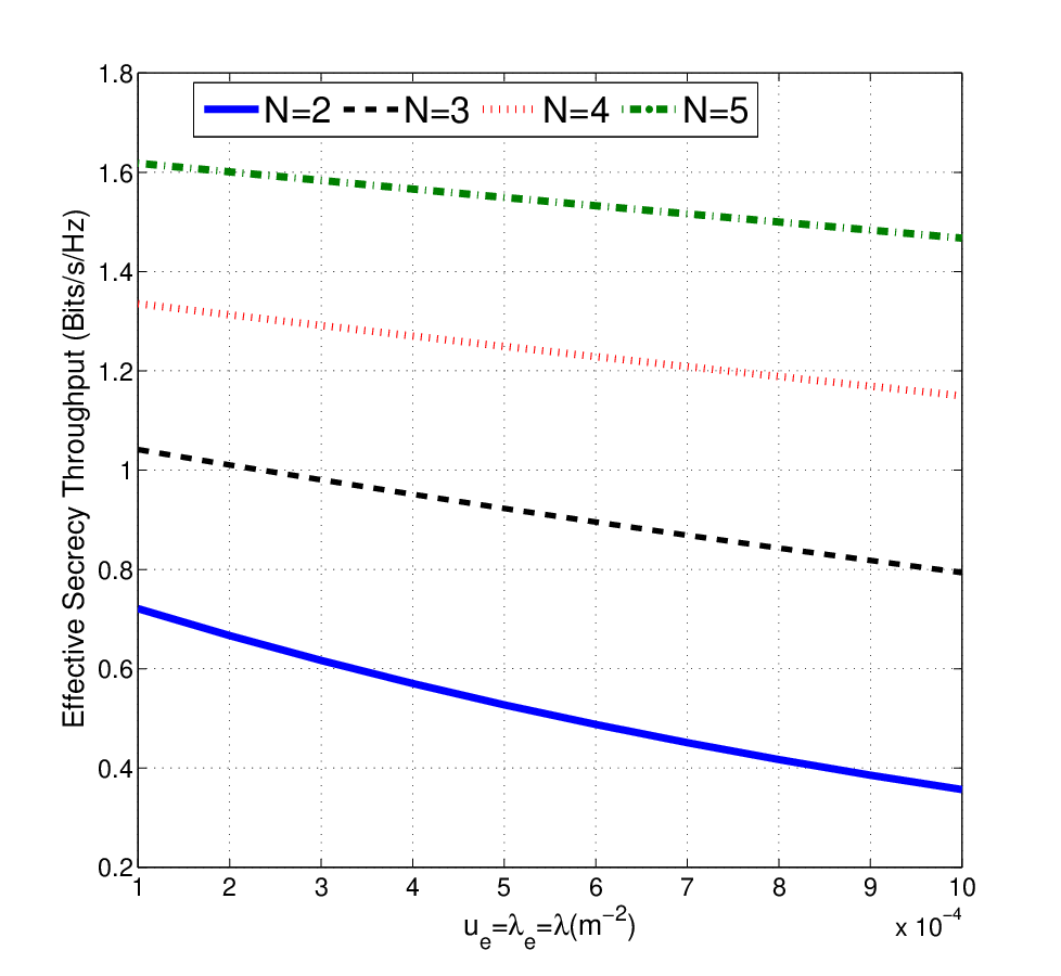
Fig. 6: The effective secrecy throughput of the typical transmitter and receiver pair versus the intensity of eavesdroppers λ\lambda for N=5,ϕ=0.6,α=2.3N=5,\phi=0.6,\alpha=2.3, λb=10−5,λl=5×10⁻⁴,ub=10−3,λe=λ,ue=5×λ\lambda_{b}=10^{-5},\lambda_{l}=5\times 10^{-4},u_{b}=10^{-3},\lambda_{e}=\lambda,u_{e}=5\times\lambda.

Fig. 6 shows the change trend of the effective secrecy throughput with the increasing intensity of Eves. Obviously, the effective secrecy throughput decreases with the increasing λ\lambda. When N=2N=2, the effective secrecy throughput decreases by 0.37 bits/s/Hz for λ\lambda changing from 10−410^{-4} to 10−310^{-3}. But, when N=5N=5, the effective secrecy throughput only decreases by about 0.15 bits/s/Hz. Then, we can make a conclusion that the decreasing rate of the effective secrecy throughput decreases with the increasing NN, and a larger antenna array can improve the robustness of the secure transmission scheme.

Fig. 7 shows the change trend of the effective secrecy throughput with the increasing number of antennas NN. Just as the simulation results in Fig. 6, more numbers of antennas employed would result in a better secrecy performance. But, the top simulation curves in Fig. 7 show that the growing rate of the effective secrecy throughput decreases when NN increases from 6 to 8. This shows that the effective secrecy throughput can not increase linearly with NN all the time and there is a best tradeoff between improving the secrecy performance and the system complexity.

Refer to caption
Fig. 7: The effective secrecy throughput of the typical transmitter and receiver pair versus the number antennas equipped at each transmitter NN for ϕ=0.6,α=2.3\phi=0.6,\alpha=2.3, λe=10−3,ue=10−2\lambda_{e}=10^{-3},u_{e}=10^{-2};
Refer to caption
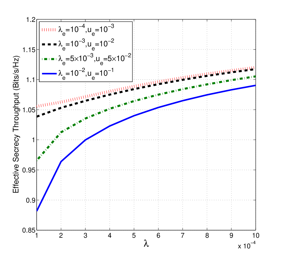
Fig. 8: The effective secrecy throughput of the typical transmitter and receiver pair versus the intensity of transmitters for N=4,λb=λN=4,\lambda_{b}=\lambda, ub=5​λu_{b}=5\lambda ϕ=0.6,α=2.3\phi=0.6,\alpha=2.3, λl=5×10⁻⁴\lambda_{l}=5\times 10^{-4}.

Fig. 8 shows the effective secrecy throughput versus the intensity of transmitters. With the increasing intensity of transmitters, the effective secrecy throughput increases, due to the decreasing distance between transmitter and receiver, and the increasing power of AN. But, from the simulation results, we can find that the secrecy performance gain obtained by increasing intensity of transmitters is small. Furthermore, when the intensity of Eves is small, the secrecy performance gains brought by making the network denser, is lower than the network with a larger intensity of Eves.

VI Conclusion

In this paper, we built a theoretical framework for analyzing the PLS of AN assisted C-V2X networks by leveraging the Cox point process. Closed-form analytical expressions of coverage probability and secrecy probability were derived, which facilitate the evaluation of the effective secrecy throughput. The simulation results show the impact of network parameters on the achievable secrecy performance. In particular, the effective secrecy throughput may be a concave/quasi-concave function of the power allocation coefficient, and the capacity for suppressing eavesdropping increases with the number of transmit antennas.

This work may have some potential extensions as follows. First, the spatial distribution of vehicles over a road is built by a static PPP model in this work. It is interesting to extend the spatial model to a stochastic geometry-based mobility model for characterizing the impact of the mobility of vehicles on the secrecy performance. Moreover, in this work, we just studied the secrecy performance of unicast communication. In practical systems, different communication modes coexist. Therefore, it is important to extend the secrecy performance analysis to a network with multiple communication modes, e.g., broadcast, unicast and multicast communications.

Appendix A Proof of Theorem 1

On the condition that the typical user is a planar node, the coverage probability in (14) is given by

p^c,p=𝔼Φb​(∑x∈ΦbPr⁡(SIRx≥γ))⏟p^c,p,1+𝔼Ψb​(∑x∈ΨbPr⁡(SIRx≥γ))⏟p^c,p,2.\displaystyle\hat{p}_{c,p}\!\!=\!\!\underset{\hat{p}_{c,p,1}}{\underbrace{\mathbb{E}_{\Phi_{b}}\left(\sum_{x\in{\Phi_{b}}}\mathrm{Pr}\left(\mathrm{SIR}_{x}\!\!\geq\!\!\gamma\right)\right)}}\!\!+\!\!\underset{\hat{p}_{c,p,2}}{\underbrace{\mathbb{E}_{\Psi_{b}}\left(\sum_{x\in{\Psi_{b}}}\mathrm{Pr}\left(\mathrm{SIR}_{x}\!\!\geq\!\!\gamma\right)\right)}}. (53)

The first part of (53), p^c,p,1\hat{p}_{c,p,1}, is the coverage probability when the typical user is associated with a planar transmitter, which can be derived as (54) at the top of the next page, where

p^c,p,1\displaystyle\hat{p}_{c,p,1} =(a)​2​π​λb​∫0+∞Pr⁡(ϕ​r−α​‖𝐟x‖F2∑y∈{Ψb+Φb}​Py​Dy​o−α≥γ)​r​𝑑r​=(b)​2​π​λb​∫0+∞∑n=0N−1[(−sp)nn!​dnd​spn​(ℒΨbc​(sp)​ℒΦbc​(sp))]sp=γ​rα​ϕ−1​r​𝑑r,\displaystyle\!\!\overset{(a)}{=}\!\!2\pi\lambda_{b}\int^{+\infty}_{0}\mathrm{Pr}\left(\frac{\phi r^{-\alpha}||\mathbf{f}_{x}||_{F}^{2}}{\underset{{y\in\left\{\Psi_{b}+\Phi_{b}\right\}}}{\sum}{P_{y}}{D^{-\alpha}_{yo}}}\!\!\geq\!\!\gamma\right)rdr\!\!\overset{(b)}{=}\!\!2\pi\lambda_{b}\int^{+\infty}_{0}\sum^{N-1}_{n=0}\left[\frac{\left(-s_{p}\right)^{n}}{n!}\frac{d^{n}}{ds_{p}^{n}}\left(\mathcal{L}^{c}_{\Psi_{b}}(s_{p})\mathcal{L}^{c}_{\Phi_{b}}(s_{p})\right)\right]_{s_{p}=\gamma r^{\alpha}\phi^{-1}}rdr, (54)


step (aa) is obtained by employing Campbell’s theorem for sums over the PPP Φb\Phi_{b} [25, Theorem 4.1] and step (bb) is due to [31, Theorem 1]. The second part of (53), p^c,p,2\hat{p}_{c,p,2}, is the coverage probability when the typical user is associated with a vehicular transmitter, which can be derived as (55) at the top of the next page.

p^c,p,2\displaystyle\hat{p}_{c,p,2} =𝔼Ξl​(∑{rb,θb}∈Ξl𝔼⁡(∑tb∈lrb,θbPr⁡(ϕ​(rb2+tb2)−α2​‖𝐟x‖F2∑y∈{Ψb+Φb+ψ⁡(lr=rb)}​Py​Dy​o−α≥γ)))\displaystyle=\mathbb{E}_{\Xi_{l}}\left(\sum_{\left\{r_{b},\theta_{b}\right\}\in\Xi_{l}}\mathbb{E}\left(\sum_{t_{b}\in l_{r_{b},\theta_{b}}}\mathrm{Pr}\left(\frac{\phi\left(r_{b}^{2}+t_{b}^{2}\right)^{-\frac{\alpha}{2}}||\mathbf{f}_{x}||_{F}^{2}}{\underset{{y\in\left\{\Psi_{b}+\Phi_{b}+\psi(l_{r=r_{b}})\right\}}}{\sum}{P_{y}}D^{-\alpha}_{yo}}\geq\gamma\right)\right)\right)
=4​λl​ub​∫0+∞d​rb​∫0+∞d​tb​∑n=0N−1[(−sv)nn!​dnd​svn​(ℒΨbc​(sv)​ℒΦbc​(sv)​ℒψb​(lr=rb)c​(sv))]sv=ϕ−1​(rb2+tb2)α2​γ.\displaystyle{=}4\lambda_{l}u_{b}\int^{+\infty}_{0}dr_{b}\int^{+\infty}_{0}dt_{b}\sum^{N-1}_{n=0}\left[\frac{\left(-s_{v}\right)^{n}}{n!}\frac{d^{n}}{ds_{v}^{n}}\left(\mathcal{L}^{c}_{\Psi_{b}}(s_{v})\mathcal{L}^{c}_{\Phi_{b}}(s_{v})\mathcal{L}^{c}_{\psi_{b}(l_{r=r_{b}})}(s_{v})\right)\right]_{s_{v}={\phi^{-1}\left(r_{b}^{2}+t_{b}^{2}\right)^{\frac{\alpha}{2}}\gamma}}. (55)


Appendix B Proof of Theorem 3

On the condition that the typical user is a vehicular node, the analytical result of the coverage probability in (14) can be derived as

p^c,v\displaystyle\hat{p}_{c,v} =𝔼Φb​(∑x∈ΦbPr⁡(SIRx≥γ))⏟p^c,v,1+𝔼Ψb​(∑x∈ΨbPr⁡(SIRx≥γ))⏟p^c,v,2\displaystyle\!=\!\underset{\hat{p}_{c,v,1}}{\underbrace{\mathbb{E}_{\Phi_{b}}\left(\sum_{x\in{\Phi_{b}}}\mathrm{Pr}\left(\mathrm{SIR}_{x}\geq\gamma\right)\right)}}\!+\!\underset{\hat{p}_{c,v,2}}{\underbrace{\mathbb{E}_{\Psi_{b}}\left(\sum_{x\in{\Psi_{b}}}\mathrm{Pr}\left(\mathrm{SIR}_{x}\geq\gamma\right)\right)}}
+𝔼ψb​(lr=0)​(∑x∈ψb​(lr=0)Pr⁡(SIRx≥γ))⏟p^c,v,3.\displaystyle\!+\!\underset{\hat{p}_{c,v,3}}{\underbrace{\mathbb{E}_{\psi_{b}(l_{r=0})}\left(\sum_{x\in{\psi_{b}(l_{r=0})}}\mathrm{Pr}\left(\mathrm{SIR}_{x}\geq\gamma\right)\right)}}. (56)

The first part of (56), p^c,v,1\hat{p}_{c,v,1}, is the coverage probability when the typical user is associated with a planar transmitter. Following the derivation in (54) and defining Ω1≜Ψb+Φb+ψ⁡(lr=0)\Omega_{1}\triangleq\Psi_{b}\!+\!\Phi_{b}\!+\!\psi\left(l_{r=0}\right), we have

p^c,v,1\displaystyle\hat{p}_{c,v,1} =2​π​λb​∫0+∞Pr⁡(ϕ​r−α​‖𝐟x‖F2∑y∈Ω1​Py​Dy​o−α≥γ)​r​𝑑r.\displaystyle\!\!=\!\!2\pi\lambda_{b}\int^{+\infty}_{0}\mathrm{Pr}\left(\frac{\phi r^{-\alpha}||\mathbf{f}_{x}||_{F}^{2}}{\underset{y\in\Omega_{1}}{\sum}{P_{y}}D^{-\alpha}_{yo}}\!\geq\!\gamma\right)rdr. (57)

The second part of (56), p^c,v,2\hat{p}_{c,v,2}, is the coverage probability when the typical user is associated with a vehicular transmitter. Following the derivation in (55) and defining Ω2≜Ψb+Φb+ψ⁡(lr=rb)+ψ⁡(lr=0)\Omega_{2}\triangleq\Psi_{b}+\Phi_{b}+\psi(l_{r=r_{b}})+\psi(l_{r=0}), we have

p^c,v,2=4​λl​ub​∫0+∞d​rb​∫0+∞Pr⁡(ϕ(rb2+tb2)α2​‖𝐟x‖F2∑y∈Ω2​Py​Dy​o−α≥γ)​d​tb.\displaystyle\hat{p}_{c,v,2}\!=\!4\lambda_{l}u_{b}\int^{+\infty}_{0}dr_{b}\int^{+\infty}_{0}\mathrm{Pr}\left(\frac{\frac{\phi}{\left(r_{b}^{2}+t_{b}^{2}\right)^{\frac{\alpha}{2}}}||\mathbf{f}_{x}||_{F}^{2}}{\underset{{y\in\Omega_{2}}}{\sum}{P_{y}}{D^{-\alpha}_{yo}}}\!\geq\!\gamma\right)dt_{b}. (58)

The third part of (56), p^c,v,3\hat{p}_{c,v,3}, is the coverage probability when the typical user is associated with a vehicular transmitter on the road lol_{o}. Employing the Campbell’s theorem for sums over the point process ψb​(lr=0)\psi_{b}\left(l_{r=0}\right) [25, Theorem 4.1] and defining Ω3≜Ψb+Φb+ψ⁡(lr=0)\Omega_{3}\triangleq\Psi_{b}+\Phi_{b}+\psi\left(l_{r=0}\right), we have

p^c,v,3\displaystyle\hat{p}_{c,v,3} =2​ub​∫0+∞Pr⁡(ϕ​tb−α​‖𝐟x‖F2∑y∈Ω3​Py​Dy​o−α≥γ)​d​tb.\displaystyle{=}2u_{b}\int^{+\infty}_{0}\mathrm{Pr}\left(\frac{\phi t_{b}^{-\alpha}||\mathbf{f}_{x}||_{F}^{2}}{\underset{{y\in\Omega_{3}}}{\sum}{P_{y}}D^{-\alpha}_{yo}}\geq\gamma\right)dt_{b}. (59)

Finally, employing Corollary 1, the exact analytical result is given as (60) at the top of the next page.

pc,p=4​λl​ub​∫0+∞d​rb​∫+∞d​tb​[∑n=0N−1(−sv)n​dnn!​d​svn​(ℒΦbc​(sv)​ℒψ⁡(lr=rb)c​(sv)​ℒψ⁡(lr=0)c​(sv)​ℒΨbc​(sv))]sv=ϕ−1​(rb2+tb2)α/2​γ\displaystyle p_{c,p}=4\lambda_{l}u_{b}\int^{+\infty}_{0}dr_{b}\int^{+\infty}dt_{b}\left[\sum^{N-1}_{n=0}\frac{\left(-s_{v}\right)^{n}d^{n}}{n!ds_{v}^{n}}\left(\mathcal{L}^{c}_{\Phi_{b}}(s_{v})\mathcal{L}^{c}_{\psi(l_{r=r_{b}})}(s_{v})\mathcal{L}^{c}_{\psi(l_{r=0})}(s_{v})\mathcal{L}^{c}_{\Psi_{b}}(s_{v})\right)\right]_{s_{v}={\phi^{-1}\left(r_{b}^{2}+t_{b}^{2}\right)^{\alpha/2}\gamma}}
+2πλb∫0+∞rdr∑n=0N−1[(−sp)nn!dnd​spn(ℒΨbc(sp)ℒψ⁡(lr=0)c(sp)ℒΦbc(sp))]sp=ϕ−1​rα​γ\displaystyle+2\pi\lambda_{b}\int^{+\infty}_{0}rdr\sum^{N-1}_{n=0}\left[\frac{\left(-s_{p}\right)^{n}}{n!}\frac{d^{n}}{ds_{p}^{n}}\left(\mathcal{L}^{c}_{\Psi_{b}}(s_{p})\mathcal{L}^{c}_{\psi(l_{r=0})}(s_{p})\mathcal{L}^{c}_{\Phi_{b}}(s_{p})\right)\right]_{s_{p}={\phi^{-1}r^{\alpha}\gamma}}
+2ub∫0+∞dtb∑n=0N−1[(−slo)nn!dnd​slon(ℒΨbc(slo)ℒψ⁡(lr=0)c(slo)ℒΦbc(slo))]slo=ϕ−1​tbα​γ.\displaystyle+2u_{b}\int^{+\infty}_{0}dt_{b}\sum^{N-1}_{n=0}\left[\frac{\left(-s_{l_{o}}\right)^{n}}{n!}\frac{d^{n}}{ds_{l_{o}}^{n}}\left(\mathcal{L}^{c}_{\Psi_{b}}(s_{l_{o}})\mathcal{L}^{c}_{\psi(l_{r=0})}(s_{l_{o}})\mathcal{L}^{c}_{\Phi_{b}}(s_{l_{o}})\right)\right]_{s_{l_{o}}={\phi^{-1}t_{b}^{\alpha}\gamma}}. (60)


Then, just as deriving the approximate result in Theorem 2, employing the lower bound on the cdf of the gamma random variable [29], the approximate result given in (25) can be obtained directly.

Appendix C Proof of Theorem 4

The secrecy probability can be expressed as

Pr(maxe∈(Φe+Ψe)SIRe≤β)=𝔼(∏e∈ΨePr⁡(SIRe≤β)⏟(I)×\displaystyle\mathrm{Pr}\left(\max_{e\in\left(\Phi_{e}+\Psi_{e}\right)}\mathrm{SIR}_{e}\leq\beta\right)=\mathbb{E}\left(\underset{(\mathrm{I})}{\underbrace{\prod_{e\in\Psi_{e}}\mathrm{Pr}\left(\mathrm{SIR}_{e}\leq\beta\right)}}\times\right.
OPEN∏e∈ΦePr⁡(SIRe≤β)⏟(II)).\displaystyle\left.\underset{(\mathrm{II})}{\underbrace{\prod_{e\in\Phi_{e}}\mathrm{Pr}\left(\mathrm{SIR}_{e}\leq\beta\right)}}\right). (61)

The expectation over the product (I)(\mathrm{I}) can be derived as (62) at the top of the next page,

𝔼(∏e∈ΨePr(SIRe≤β))=(a)𝔼(∏(re,θe)∈Ξl𝔼(∏te∈ψ⁡(lre,θe)Pr(ϕ​|qe|2​(re2+te2)−α2(1−ϕ)​‖𝐠o​e‖F2​(re2+te2)−α2N−1+∑x∈Δb,p​(1−u)​‖𝐠x​e‖F2​Dx​e−αN−1≤β|Δb,p)))\displaystyle\mathbb{E}\left(\prod_{e\in\Psi_{e}}\mathrm{Pr}\left(\mathrm{SIR}_{e}\leq\beta\right)\right)\!\!\overset{(a)}{=}\!\!\mathbb{E}\left(\prod_{(r_{e},\theta_{e})\in\Xi_{l}}\mathbb{E}\left(\prod_{t_{e}\in\psi(l_{r_{e},\theta_{e}})}\mathrm{Pr}\left(\left.\frac{\phi|q_{e}|^{2}\left(r_{e}^{2}+t_{e}^{2}\right)^{-\frac{\alpha}{2}}}{\frac{(1-\phi)||\mathbf{g}_{oe}||_{F}^{2}\left(r_{e}^{2}+t_{e}^{2}\right)^{-\frac{\alpha}{2}}}{N-1}+\underset{{x\in\Delta_{b,p}}}{\sum}\frac{(1-u)||\mathbf{g}_{xe}||_{F}^{2}D_{xe}^{-\alpha}}{N-1}}\!\!\leq\!\!\beta\right|\Delta_{b,p}\right)\right)\right)
=(b)𝔼(exp(−λlπ∫02​πdθe∫0+∞dree−2ue∫+∞0Pr(ϕ⁡(N−1)1−ϕ​|qe|2​(re2+te2)−α2‖𝐠o​e‖F2​(re2+te2)−α2+∑x∈Δb,p​‖𝐠x​e‖F2​Dx​e−α≥β|Δb,p)dte))\displaystyle\overset{(b)}{=}\mathbb{E}\left(\mathrm{exp}\left(-\frac{\lambda_{l}}{\pi}\int^{2\pi}_{0}d\theta_{e}\int^{+\infty}_{0}dr_{e}\mathrm{e}^{-2u_{e}\int^{+\infty}_{0}\mathrm{Pr}\left(\left.\frac{\frac{\phi\left(N-1\right)}{1-\phi}|q_{e}|^{2}\left(r_{e}^{2}+t_{e}^{2}\right)^{-\frac{\alpha}{2}}}{||\mathbf{g}_{oe}||_{F}^{2}\left(r_{e}^{2}+t_{e}^{2}\right)^{-\frac{\alpha}{2}}+\underset{{x\in\Delta_{b,p}}}{\sum}||\mathbf{g}_{xe}||_{F}^{2}D_{xe}^{-\alpha}}\geq\beta\right|\Delta_{b,p}\right)dt_{e}}\right)\right)
⪆(c)exp(−2λl∫0+∞dree−2ue∫+∞0Pr(ϕ⁡(N−1)1−ϕ​|qe|2​(re2+te2)−α2‖𝐠o​e‖F2​(re2+te2)−α2+∑x∈Δb,p​‖𝐠x​e‖F2​Dx​e−α≥β)dte),\displaystyle\overset{(c)}{\gtrapprox}\mathrm{exp}\left(-{2\lambda_{l}}\int^{+\infty}_{0}dr_{e}\mathrm{e}^{-2u_{e}\int^{+\infty}_{0}\mathrm{Pr}\left(\frac{\frac{\phi\left(N-1\right)}{1-\phi}|q_{e}|^{2}\left(r_{e}^{2}+t_{e}^{2}\right)^{-\frac{\alpha}{2}}}{||\mathbf{g}_{oe}||_{F}^{2}\left(r_{e}^{2}+t_{e}^{2}\right)^{-\frac{\alpha}{2}}+\underset{{x\in\Delta_{b,p}}}{\sum}||\mathbf{g}_{xe}||_{F}^{2}D_{xe}^{-\alpha}}\geq\beta\right)dt_{e}}\right), (62)


where Δb,p≜Φb∪Ψb∪ψb​(le)\Delta_{b,p}\triangleq{\Phi_{b}\cup\Psi_{b}\cup\psi_{b}(l_{e})}. At step (a)(a), the distance between the typical planar transmitter and the vehicular Eve is re2+te2\sqrt{r_{e}^{2}+t_{e}^{2}}, which is illustrated in Fig. 1, where rer_{e} is the perpendicular distance from the typical transmitter located at the origin to the road, and tet_{e} denotes the distance of the vehicular Eve from the projection of the origin onto the road, i.e., o′o^{\prime}. Notice that under the condition that e∈Ψee\in\Psi_{e}, the eavesdropper is on a road which is denoted as lel_{e} and the corresponding point on the representation space is denoted as (re,θe)(r_{e},\theta_{e}). Therefore, for each vehicular Eve at e∈Ψee\in\Psi_{e}, the interference received at Eve comes from multiple planar transmitters, vehicular transmitters on the road lel_{e}, and vehicular transmitters on the other roads. Step (b)(b) is obtained by using the PGFL of the point process ψ⁡(lre,θe)\psi(l_{r_{e},\theta_{e}}) and the point process Ξl\Xi_{l} [25, Theorem 4.9]. Step (cc) is due to the Jensen’s inequality.

Employing the PGFL of Φe\Phi_{e}, the expectation over the product (II)(\mathrm{II}) can be derived as

𝔼⁡(∏e∈ΦePr⁡(SIRe≤β))=\displaystyle\mathbb{E}\left(\prod_{e\in\Phi_{e}}\mathrm{Pr}\left(\mathrm{SIR}_{e}\leq\beta\right)\right){=}
e−2λeπ∫0+∞Pr(ϕ⁡(N−1)1−ϕ​|qe|2​re−α‖𝐠o​e‖F2​re−α+∑x∈{Φb+Ψb}​‖𝐠x​e‖F2​Dx​e−α≥β)redre.\displaystyle e^{-2\lambda_{e}\pi\int_{0}^{+\infty}\mathrm{Pr}\left(\frac{\frac{\phi(N-1)}{1-\phi}|q_{e}|^{2}r_{e}^{-{\alpha}}}{||\mathbf{g}_{oe}||_{F}^{2}r_{e}^{-{\alpha}}+\underset{{x\in\{\Phi_{b}+\Psi_{b}\}}}{\sum}{||\mathbf{g}_{xe}||_{F}^{2}D_{xe}^{-\alpha}}}\geq\beta\right)r_{e}dr_{e}}. (63)

Since the planar Eve does not have to locate at any road, the planar Eve only suffers the interference from the transmitters at Φb∪Ψb\Phi_{b}\cup\Psi_{b}.

For obtaining the secrecy probability, the complementary cumulative distribution function (ccdf) of the SIR received by Eve should be derived first. Defining s≜(ϕ−1−1)​βN−1s\triangleq\frac{(\phi^{-1}-1)\beta}{N-1}, the ccdf in (62) is given as (64) at the top of the next page.

Pr⁡(ϕ​|qe|2​(re2+te2)−α21−ϕ(N−1)​(re2+te2)α2​‖𝐠o​e‖F2+∑x∈{Φb+Ψb+ψ⁡(le)}​(1−ϕ)​‖𝐠x​e‖F2​Dx​e−α(N−1)≥β)​=(a)​exp⁡(−(s​(re2+te2)α2​∑x∈{Φb+Ψb+ψ⁡(le)}​‖𝐠x​e‖F2​Dx​e−α))(1+β​ϕ−1−1N−1)N−1\displaystyle\mathrm{Pr}\left(\frac{\phi|q_{e}|^{2}\left(r_{e}^{2}+t_{e}^{2}\right)^{-\frac{\alpha}{2}}}{\frac{1-\phi}{\left(N-1\right)\left(r_{e}^{2}+t_{e}^{2}\right)^{\frac{\alpha}{2}}}||\mathbf{g}_{oe}||_{F}^{2}+\underset{{x\in\{\Phi_{b}+\Psi_{b}+\psi(l_{e})\}}}{\sum}\frac{(1-\phi)||\mathbf{g}_{xe}||_{F}^{2}D_{xe}^{-\alpha}}{(N-1)}}\geq\beta\right)\overset{(a)}{=}\frac{\mathrm{exp}\left(-\left(s\left(r_{e}^{2}+t_{e}^{2}\right)^{\frac{\alpha}{2}}\underset{{x\in\{\Phi_{b}+\Psi_{b}+\psi(l_{e})\}}}{\sum}||\mathbf{g}_{xe}||_{F}^{2}D_{xe}^{-\alpha}\right)\right)}{\left(1+\beta\frac{\phi^{-1}-1}{N-1}\right)^{N-1}}
=(b)​(1+β​ϕ−1−1N−1)1−N​ℒΦbs​(s​(re2+te2)α2)(i)​ℒΨbs​(s​(re2+te2)α2)(ii)​ℒψb​(lr=0)s​(s​(re2+te2)α2)(iii).\displaystyle\overset{(b)}{=}\left(1+\beta\frac{\phi^{-1}-1}{N-1}\right)^{1-N}\underset{(\mathrm{i})}{{\mathcal{L}^{s}_{\Phi_{b}}\left(s\left(r_{e}^{2}+t_{e}^{2}\right)^{\frac{\alpha}{2}}\right)}}\underset{(\mathrm{ii})}{\mathcal{L}^{s}_{\Psi_{b}}\left(s\left(r_{e}^{2}+t_{e}^{2}\right)^{\frac{\alpha}{2}}\right)}\underset{(\mathrm{iii})}{\mathcal{L}^{s}_{\psi_{b}(l_{r=0})}\left(s\left(r_{e}^{2}+t_{e}^{2}\right)^{\frac{\alpha}{2}}\right)}. (64)


Step (a)(a) is due to the Laplace transform of the gamma random variable, and step (b)(b) is due to that Φb\Phi_{b}, Ψb\Psi_{b}, and ψ⁡(lr=0)\psi(l_{r=0}) are all independent.

Applying Corollary 3, Laplace transforms (i)-(iii) in (64) can be derived. Substituting the analytical result of (64) into (62), the analytical result of 𝔼⁡(∏e∈Ψe​Pr​(SIRe≤β))\mathbb{E}\left(\underset{{e\in\Psi_{e}}}{\prod}\mathrm{Pr}\left(\mathrm{SIR}_{e}\leq\beta\right)\right) can be obtained. With the same procedures, the analytical result of 𝔼⁡(∏e∈Φe​Pr​(SIRe≤β))\mathbb{E}\left(\underset{{e\in\Phi_{e}}}{\prod}\mathrm{Pr}\left(\mathrm{SIR}_{e}\leq\beta\right)\right) can be obtained. Then, the secrecy probability can be derived with (61).

Appendix D Proof of Theorem 5

On the condition that the typical transmitter is a planar node, the secrecy probability is derived by considering two events: 1) the nearest Eve is a vehicular node, which is denoted by ε0,p\varepsilon_{0,p}; 2) the nearest Eve is a planar node, which is denoted as ε1,p\varepsilon_{1,p}. Then, considering the nearest Eve only, the secrecy probability ps​e​c,pLp_{sec,p}^{L} can be established as (65) at the previous page.

ps​e​c,pL\displaystyle p_{sec,p}^{L} =𝔼de∗​(Pr⁡(ϕ​|qe|2​(de∗)−α(1−ϕ)​‖𝐠o​e‖F2​(de∗)−αN−1+∑x∈{Φb+Ψb+ψb​(le)}​(1−ϕ)​‖𝐠x​e‖F2​Dx​e−αN−1≤β,ε0,p))⏟ps​e​c,p,1L\displaystyle=\underset{p_{sec,p,1}^{L}}{\underbrace{\mathbb{E}_{d_{e}^{*}}\left(\mathrm{Pr}\left(\frac{\phi|q_{e}|^{2}\left({d^{*}_{e}}\right)^{-\alpha}}{\frac{(1-\phi)||\mathbf{g}_{oe}||_{F}^{2}\left({d^{*}_{e}}\right)^{-\alpha}}{N-1}+\underset{{x\in\left\{\Phi_{b}+\Psi_{b}+\psi_{b}(l_{e})\right\}}}{\sum}\frac{(1-\phi)||\mathbf{g}_{xe}||_{F}^{2}D_{xe}^{-\alpha}}{N-1}}\leq\beta,\varepsilon_{0,p}\right)\right)}}
+𝔼de∗​(Pr⁡(ϕ​|qe|2​(de∗)−α(1−ϕ)​‖𝐠o​e‖F2​(de∗)−αN−1+∑x∈{Φb+Ψb}​(1−ϕ)​‖𝐠x​e‖F2​Dx​e−αN−1≤β,ε1,p))⏟ps​e​c,p,2L.\displaystyle+\underset{p_{sec,p,2}^{L}}{\underbrace{\mathbb{E}_{d^{*}_{e}}\left(\mathrm{Pr}\left(\frac{\phi|q_{e}|^{2}\left({d^{*}_{e}}\right)^{-\alpha}}{\frac{(1-\phi)||\mathbf{g}_{oe}||_{F}^{2}\left({d^{*}_{e}}\right)^{-\alpha}}{N-1}+\underset{{x\in\left\{\Phi_{b}+\Psi_{b}\right\}}}{\sum}\frac{(1-\phi)||\mathbf{g}_{xe}||_{F}^{2}D_{xe}^{-\alpha}}{N-1}}\leq\beta,\varepsilon_{1,p}\right)\right)}}. (65)


Let’s derive the first expectation ps​e​c,v,1Lp_{sec,v,1}^{L} in (65).

ps​e​c,p,1L=∫0+∞(1−ℒΨbs​(s​τα)​ℒΦbs​(s​τα)​ℒψb​(lr=0)s​(s​τα)(1+s)N−1)\displaystyle p_{sec,p,1}^{L}=\!\!\int^{+\infty}_{0}\!\!\left(1-\frac{\mathcal{L}^{s}_{\Psi_{b}}\left({s\tau^{\alpha}}\right)\mathcal{L}^{s}_{\Phi_{b}}\left({s\tau^{\alpha}}\right)\mathcal{L}^{s}_{\psi_{b}(l_{r=0})}\left({s\tau^{\alpha}}\right)}{\left(1+s\right)^{N-1}}\right)
×fde∗,ε0,p​(τ)​d​τ,\displaystyle\times f_{d^{*}_{e},\varepsilon_{0,p}}(\tau)\mathrm{d}\tau, (66)

where fde∗,ε0,p​(τ)f_{d^{*}_{e},\varepsilon_{0,p}}(\tau) is given in (32). With Corollary 3, the analytical result of ps​e​c,v,1Lp_{sec,v,1}^{L} can be obtained. Second, let’s derive the second expectation ps​e​c,p,2Lp_{sec,p,2}^{L} in (65).

ps​e​c,p,2L=\displaystyle p_{sec,p,2}^{L}= ∫0+∞(1−ℒΨbs​(s​τα)​ℒΦbs​(s​τα)(1+s)N−1)​fde∗,ε1,p​(τ)​𝑑τ,\displaystyle\int^{+\infty}_{0}\left(1-\frac{\mathcal{L}^{s}_{\Psi_{b}}\left({s\tau^{\alpha}}\right)\mathcal{L}^{s}_{\Phi_{b}}\left({s\tau^{\alpha}}\right)}{\left(1+s\right)^{N-1}}\right)f_{d^{*}_{e},\varepsilon_{1,p}}(\tau)\mathrm{d}\tau, (67)

where fde∗,ε1,p​(τ)f_{d^{*}_{e},\varepsilon_{1,p}}(\tau) has been given in (33). Employing Corollary 3, the analytical result of ps​e​c,p,2Lp_{sec,p,2}^{L} can be obtained. Finally substituting (66) and (67) into (65), the analytical result of ps​e​c,pLp_{sec,p}^{L} can be obtained.

Appendix E Proof of Theorem 6

The secrecy probability is

Pr(maxe∈(Φe+Ψe+ψe​(lo))SIRe≤β)=𝔼(∏e∈ΨePr⁡(SIRe≤β)⏟(I)×\displaystyle\mathrm{Pr}\left(\max_{e\in\left(\Phi_{e}+\Psi_{e}+\psi_{e}(l_{o})\right)}\mathrm{SIR}_{e}\!\leq\!\beta\right)\!\!=\!\!\mathbb{E}\left(\underset{(\mathrm{I})}{\underbrace{\prod_{e\in\Psi_{e}}\mathrm{Pr}\left(\mathrm{SIR}_{e}\!\!\leq\!\!\beta\right)}}\times\right.
OPEN∏e∈ΦePr⁡(SIRe≤β)⏟(II)​∏e∈ψe​(lo)Pr⁡(SIRe≤β)⏟(III)).\displaystyle\left.\underset{(\mathrm{II})}{\underbrace{\prod_{e\in\Phi_{e}}\mathrm{Pr}\left(\mathrm{SIR}_{e}\!\!\leq\!\!\beta\right)}}\underset{(\mathrm{III})}{\underbrace{\prod_{e\in\psi_{e}(l_{o})}\mathrm{Pr}\left(\mathrm{SIR}_{e}\!\!\leq\!\!\beta\right)}}\right). (68)
Refer to caption
(a) θ>π2\theta>\frac{\pi}{2}
Refer to caption
(b) θ<π2\theta<\frac{\pi}{2}.
Fig. 9: Illustration of the relative location, where o′o^{\prime} is the projection of the origin oo onto the road lel_{e} and o^\hat{o} is the projection of the vehicular Eve’s location onto the road lol_{o}. h⁡(θe)h(\theta_{e}) is the perpendicular distance from the vehicular Eve to the road lol_{o}.

Following the procedures in (62), a lower bound on the expectation over the product (I)(\mathrm{I}) in (68) can be derived as (69) at the top of the next page,

𝔼(∏e∈ΨePr(SIRe≤β))⪆exp(−λlπ∫02​πdθe∫0+∞dree−ue∫+∞−∞Pr(ϕ⁡(N−1)1−ϕ​|qe|2​(re2+te2)−α2‖𝐠o​e‖F2​(re2+te2)−α2+∑x∈Δb,v​‖𝐠x​e‖F2​Dx​e−α≥β)dte),\displaystyle\mathbb{E}\left(\prod_{e\in\Psi_{e}}\mathrm{Pr}\left(\mathrm{SIR}_{e}\leq\beta\right)\right){\gtrapprox}\mathrm{exp}\left(-\frac{\lambda_{l}}{\pi}\int^{2\pi}_{0}d\theta_{e}\int^{+\infty}_{0}dr_{e}\mathrm{e}^{-u_{e}\int^{+\infty}_{-\infty}\mathrm{Pr}\left(\frac{\frac{\phi\left(N-1\right)}{1-\phi}|q_{e}|^{2}\left(r_{e}^{2}+t_{e}^{2}\right)^{-\frac{\alpha}{2}}}{||\mathbf{g}_{oe}||_{F}^{2}\left(r_{e}^{2}+t_{e}^{2}\right)^{-\frac{\alpha}{2}}+\underset{{x\in\Delta_{b,v}}}{\sum}||\mathbf{g}_{xe}||_{F}^{2}D_{xe}^{-\alpha}}\geq\beta\right)dt_{e}}\right), (69)


where Δb,v≜Φb∪Ψb∪ψb​(le)∪ψb​(lo)\Delta_{b,v}\triangleq{\Phi_{b}\cup\Psi_{b}\cup\psi_{b}(l_{e})\cup\psi_{b}(l_{o})}.

Employing the PGFL of Φe\Phi_{e}, a lower bound on the expectation over the product (II)(\mathrm{II}) in (68) is given by

𝔼⁡(∏e∈ΦePr⁡(SIRe≤β))⪆\displaystyle\mathbb{E}\left(\prod_{e\in\Phi_{e}}\mathrm{Pr}\left(\mathrm{SIR}_{e}\leq\beta\right)\right){\gtrapprox}
e−2λeπ∫0+∞Pr(ϕ⁡(N−1)1−ϕ​|qe|2​re−α‖𝐠o​e‖F2reα+∑x∈{Φb+Ψb+ψb​(lo)}​‖𝐠x​e‖F2Dx​eα≥β)redre.\displaystyle e^{-2\lambda_{e}\pi\int_{0}^{+\infty}\mathrm{Pr}\left(\frac{\frac{\phi(N-1)}{1-\phi}|q_{e}|^{2}r_{e}^{-{\alpha}}}{\frac{||\mathbf{g}_{oe}||_{F}^{2}}{r_{e}^{{\alpha}}}+\underset{{x\in\{\Phi_{b}+\Psi_{b}+\psi_{b}(l_{o})\}}}{\sum}\frac{||\mathbf{g}_{xe}||_{F}^{2}}{D_{xe}^{\alpha}}}\geq\beta\right)r_{e}dr_{e}}. (70)

Employing the PGFL of ψe​(lo)\psi_{e}\left(l_{o}\right), a lower bound on the expectation over the product (III)(\mathrm{III}) in (68) can be derived as

𝔼⁡(∏e∈ψe​(lo)Pr⁡(SIRe≤β))⪆\displaystyle\mathbb{E}\left(\prod_{e\in\psi_{e}(l_{o})}\mathrm{Pr}\left(\mathrm{SIR}_{e}\leq\beta\right)\right){\gtrapprox}
e−2ue∫0+∞Pr(ϕ⁡(N−1)1−ϕ​|qe|2​te−α‖𝐠o​e‖F2teα+∑x∈{Φb+Ψb+ψb​(lo)}​‖𝐠x​e‖F2Dx​eα≥β)dte.\displaystyle e^{-2u_{e}\int_{0}^{+\infty}\mathrm{Pr}\left(\frac{\frac{\phi(N-1)}{1-\phi}|q_{e}|^{2}t_{e}^{-{\alpha}}}{\frac{||\mathbf{g}_{oe}||_{F}^{2}}{t_{e}^{{\alpha}}}+\underset{{x\in\{\Phi_{b}+\Psi_{b}+\psi_{b}(l_{o})\}}}{\sum}\frac{||\mathbf{g}_{xe}||_{F}^{2}}{D_{xe}^{\alpha}}}\geq\beta\right)dt_{e}}. (71)

Notice that under the condition that e∈ψe​(lo)e\in\psi_{e}(l_{o}), the eavesdroppers are on the same road as the typical vehicular transmitter. Therefore, such eavesdroppers would suffer the interference from the transmitters at Φb∪Ψb∪ψb​(lo)\Phi_{b}\cup\Psi_{b}\cup\psi_{b}(l_{o}).

For obtaining the analytical result of the secrecy probability, the ccdf of the SIR received by Eve should be derived first.

Defining s≜(ϕ−1−1)​(re2+te2)α2​βN−1s\triangleq\frac{(\phi^{-1}-1)\left(r_{e}^{2}+t_{e}^{2}\right)^{\frac{\alpha}{2}}\beta}{N-1}, and following the procedures in (64), the ccdf in (69) can be derived as (72) at the top of the next page,

Pr⁡(ϕ​|qe|2​(re2+te2)−α2(1−ϕ)​‖𝐠o​e‖F2(N−1)​(re2+te2)α2+∑x∈{Φb+Ψb+ψb​(le)+ψb​(lo)}​(1−u)​‖𝐠x​e‖F2​Dx​e−α(N−1)≥β)=ℒΦbs​(s)(i)​ℒΨbs​(s)(ii)​ℒψb​(lr=0)s​(s)(iii)​ℒψb​(lr=h⁡(θe))s​(s)(iv)(1+β​ϕ−1−1N−1)N−1,\displaystyle\mathrm{Pr}\left(\frac{\phi|q_{e}|^{2}\left(r_{e}^{2}+t_{e}^{2}\right)^{-\frac{\alpha}{2}}}{\frac{\left(1-\phi\right)||\mathbf{g}_{oe}||_{F}^{2}}{\left(N-1\right)\left(r_{e}^{2}+t_{e}^{2}\right)^{\frac{\alpha}{2}}}+\underset{{x\in\{\Phi_{b}+\Psi_{b}+\psi_{b}(l_{e})+\psi_{b}(l_{o})\}}}{\sum}\frac{(1-u)||\mathbf{g}_{xe}||^{2}_{F}D_{xe}^{-\alpha}}{(N-1)}}\geq\beta\right){=}\frac{\overset{(\mathrm{i})}{{\mathcal{L}^{s}_{\Phi_{b}}(s)}}\overset{(\mathrm{ii})}{\mathcal{L}^{s}_{\Psi_{b}}(s)}\overset{(\mathrm{iii})}{\mathcal{L}^{s}_{\psi_{b}(l_{r=0})}(s)}\overset{(\mathrm{iv})}{\mathcal{L}^{s}_{\psi_{b}(l_{r=h(\theta_{e})})}(s)}}{\left(1+\beta\frac{\phi^{-1}-1}{N-1}\right)^{N-1}}, (72)


where h⁡(θe)h(\theta_{e}) is the perpendicular distance from the vehicular Eve to lol_{o}, as illustrated in Fig. 9.

Applying Corollary 3, the analytical results of the Laplace transforms (i)-(iii) in (72) can be obtained. For deriving the Laplace transform (iv) in (72), h⁡(θe)h(\theta_{e}) should be derived firstly. As illustrated in Fig. 9, h⁡(θe)=re​sin​(θe)−te​cos​(θe)h(\theta_{e})=r_{e}\mathrm{sin}(\theta_{e})-t_{e}\mathrm{cos}(\theta_{e}), where te>0t_{e}>0 when the vehicular Eve is at the right of o′o^{\prime}, otherwise, te<0t_{e}<0. Employing Corollary 3, the analytical result of ℒψb​(lr=h⁡(θe))s​(s)\mathcal{L}^{s}_{\psi_{b}(l_{r=h(\theta_{e})})}(s) can be obtained. Then, substituting (72) into (69), the analytical result of 𝔼⁡(∏e∈Ψe​Pr​(SIRe≤β))\mathbb{E}\left(\underset{{e\in\Psi_{e}}}{\prod}\mathrm{Pr}\left(\mathrm{SIR}_{e}\leq\beta\right)\right) can be obtained.

With similar procedures, the analytical results of ∏e∈Φe​Pr​(SIRe≤β){\underset{{e\in\Phi_{e}}}{\prod}\mathrm{Pr}\left(\mathrm{SIR}_{e}\leq\beta\right)} and ∏e∈ψe​(lo)​Pr​(SIRe≤β){\underset{{e\in\psi_{e}(l_{o})}}{\prod}\mathrm{Pr}\left(\mathrm{SIR}_{e}\leq\beta\right)} can be obtained and the detailed derivations are omitted due to the space limitation. Substituting (69), (70) and (71) into (68), a lower bound on the secrecy probability can be obtained.

References

  • [1] H. Seo, K. Lee, S. Yasukawa, Y. Peng, and P. Sartori, “LTE evolution for vehicle-to-everything services,” IEEE Communications Magazine, vol. 54, no. 6, pp. 22–28, Jun. 2016.
  • [2] V. Marojevic, “C-V2X security requirements and procedures: survey and research directions,” arXiv preprint 2018. [Online]. Available: https://arxiv.org/ftp/arxiv/papers/1807/1807.09338.pdf
  • [3] V. Marojevic, C. Kamhoua, J. Reed, and F. Jondral, “Secure wireless communications for vehicle-to-everything,” IEEE Communications Magazine, vol. 57, no. 10, pp. 76–76, 2019.
  • [4] Y. Zou, J. Zhu, X. Wang, and L. Hanzo, “A survey on wireless security: technical challenges, recent advances, and future trends,” Proceedings of the IEEE, vol. 104, no. 9, pp. 1727–1765, Sep. 2016.
  • [5] M. N. Mejri, J. Ben-Othman, and M. Hamdi, “Survey on VANET security challenges and possible cryptographic solutions,” Vehicular Communications, vol. 1, no. 2, pp. 53 – 66, 2014. [Online]. Available: http://www.sciencedirect.com/science/article/pii/S2214209614000187
  • [6] D. W. K. Ng, E. S. Lo, and R. Schober, “Multiobjective resource allocation for secure communication in cognitive radio networks with wireless information and power transfer,” IEEE Transactions on Vehicular Technology, vol. 65, no. 5, pp. 3166–3184, 2016.
  • [7] H. M. Furqan, M. S. J. Solaija, and H. Arslan, “Intelligent physical layer security approach for V2X communication,” arXiv preprint, 2019. [Online]. Available: https://arxiv.org/pdf/1905.05075.pdf
  • [8] N.-Y. Ahn, D. Lee, and S.-J. Oh, “Vehicle communication using secrecy capacity,” arXiv preprint, 2019. [Online]. Available: https://arxiv.org/ftp/arxiv/papers/1807/1807.09757.pdf
  • [9] X. Luo, Y. Liu, H. Chen, and Q. Guo, “Physical layer security in intelligently connected vehicle networks,” IEEE Network, to be published, doi: https://doi.org/10.1109/MNET.011.1900628, 2020.
  • [10] M. Mosca, “Cybersecurity in an era with quantum computers: Will we be ready?” IEEE Security Privacy, vol. 16, no. 5, pp. 38–41, 2018.
  • [11] Y. Liu, W. Wang, H. Chen, L. Wang, N. Cheng, W. Meng, and X. Shen, “Secrecy rate maximization via radio resource allocation in cellular underlaying V2V communications,” IEEE Transactions on Vehicular Technology, to be published, doi: https://doi.org/10.1109/TVT.2020.2986088, 2020.
  • [12] Y. Liu, H. Chen, and L. Wang, “Physical layer security for next generation wireless networks: Theories, technologies, and challenges,” IEEE Communications Surveys Tutorials, vol. 19, no. 1, pp. 347–376, 2017.
  • [13] “Study on LTE-based V2X services,” 3GPP TR 36.885, Tech. Rep., Jul. 2018.
  • [14] M. Haenggi, J. G. Andrews, F. Baccelli, O. Dousse, and M. Franceschetti, “Stochastic geometry and random graphs for the analysis and design of wireless networks,” IEEE Journal Selected Areas in Communications, vol. 27, no. 7, pp. 1029–1046, Sep. 2009.
  • [15] C. Choi and F. Baccelli, “Poisson Cox point processes for vehicular networks,” IEEE Transactions on Vehicular Technology, vol. 67, no. 10, pp. 10 160–10 165, Oct. 2018.
  • [16] Y. Wang, K. Venugopal, A. F. Molisch, and R. W. Heath, “Mmwave vehicle-to-infrastructure communication: Analysis of urban microcellular networks,” IEEE Transactions on Vehicular Technology, vol. 67, no. 8, pp. 7086–7100, 2018.
  • [17] C. Choi and F. Baccelli, “An analytical framework for coverage in cellular networks leveraging vehicles,” IEEE Transactions on Communications, vol. 66, no. 10, pp. 4950–4964, Oct. 2018.
  • [18] X. Zhang, X. Zhou, and M. R. McKay, “Enhancing secrecy with multi-antenna transmission in wireless ad hoc networks,” IEEE Transactions on Information Forensics and Security, vol. 8, no. 11, pp. 1802–1814, Nov. 2013.
  • [19] C. Wang and H. Wang, “Physical layer security in millimeter wave cellular networks,” IEEE Transactions on Wireless Communications, vol. 15, no. 8, pp. 5569–5585, Aug. 2016.
  • [20] H. S. Dhillon, R. K. Ganti, F. Baccelli, and J. G. Andrews, “Modeling and analysis of K-tier downlink heterogeneous cellular networks,” IEEE Journal on Selected Areas in Communications, vol. 30, no. 3, pp. 550–560, Apr. 2012.
  • [21] Y. Liu, H. Chen, L. Wang, and W. Meng, “Artificial noisy MIMO systems under correlated scattering rayleigh fading — a physical layer security approach,” IEEE Systems Journal, vol. 14, no. 2, pp. 2121–2132, 2020.
  • [22] A. D. Wyner, “The wire-tap channel,” The Bell System Technical Journal, vol. 54, no. 8, pp. 1355–1387, Oct. 1975.
  • [23] X. Zhou, M. R. McKay, B. Maham, and A. Hjorungnes, “Rethinking the secrecy outage formulation: a secure transmission design perspective,” IEEE Wireless Communications Letters, vol. 15, no. 3, pp. 302–304, Mar. 2011.
  • [24] S. Yan, N. Yang, G. Geraci, R. Malaney, and J. Yuan, “Optimization of code rates in SISOME wiretap channels,” IEEE Transactions on Wireless Communications, vol. 14, no. 11, pp. 6377–6388, Nov. 2015.
  • [25] M. Haenggi, Stochastic Geometry for Wireless Network. Cambridge, U.K.: Cambridge Univ. Press, 2012.
  • [26] P. Loya, Amazing and aesthetic aspects of analysis. Springer, 2017.
  • [27] M. Haenggi, J. G. Andrews, F. Baccelli, O. Dousse, and M. Franceschetti, “Stochastic geometry and random graphs for the analysis and design of wireless networks,” IEEE Journal on Selected Areas in Communications, vol. 27, no. 7, pp. 1029–1046, 2009.
  • [28] R. J. Muirhead, Aspects of Multivariate Statistical Theory. Hoboken, New Jersey, USA: John Wiley & Sons, Inc.,, 1982.
  • [29] H. Alzer, “On some inequalities for the incomplete gamma function,” Mathematics of Computation of the American Mathematical Society, vol. 66, no. 218, pp. 771–778, 1997.
  • [30] I. S. Gradshteyn and I. M. Ryzhik, Table of integrals, series, and products. Academic press, 2014.
  • [31] A. M. Hunter, J. G. Andrews, and S. Weber, “Transmission capacity of ad hoc networks with spatial diversity,” IEEE Transactions on Wireless Communications, vol. 7, no. 12, pp. 5058–5071, Dec. 2008.