A law of robustness for two-layers neural networks
Abstract
We initiate the study of the inherent tradeoffs between the size of a neural network and its robustness, as measured by its Lipschitz constant. We make a precise conjecture that, for any Lipschitz activation function and for most datasets, any two-layers neural network with neurons that perfectly fit the data must have its Lipschitz constant larger (up to a constant) than where is the number of datapoints. In particular, this conjecture implies that overparametrization is necessary for robustness, since it means that one needs roughly one neuron per datapoint to ensure a -Lipschitz network, while mere data fitting of -dimensional data requires only one neuron per datapoints. We prove a weaker version of this conjecture when the Lipschitz constant is replaced by an upper bound on it based on the spectral norm of the weight matrix. We also prove the conjecture in the high-dimensional regime (which we also refer to as the undercomplete case, since only is relevant here). Finally we prove the conjecture for polynomial activation functions of degree when . We complement these findings with experimental evidence supporting the conjecture.
1 Introduction
We study two-layers neural networks with inputs in , neurons, and Lipschitz non-linearity . These are functions of the form:
| (1) |
with and for any . We denote by the set of functions of the form (1). When is large enough and is non-polynomial, this set of functions can be used to fit any given data set (Cybenko 1989; Leshno et al. 1993). That is, given a data set , one can find such that
| (2) |
In a variety of scenarios one is furthermore interested in fitting the data smoothly. For example, in machine learning, the data fitting model is used to make predictions at unseen points . It is reasonable to ask for these predictions to be stable, that is a small perturbation of should result in a small perturbation of .
A natural question is: how “costly” is this stability restriction compared to mere data fitting? In practice it seems much harder to find robust models for large scale problems, as first evidenced in the seminal paper (Szegedy et al. 2013). In theory the “cost” of finding robust models has been investigated from a computational complexity perspective in (Bubeck et al. 2019), from a statistical perspective in (Schmidt et al. 2018), and more generally from a model complexity perspective in (Degwekar et al. 2019; Raghunathan et al. 2019; Allen-Zhu and Li 2020). We propose here a different angle of study within the broad model complexity perspective: does a model have to be larger for it to be robust? Empirical evidence (e.g., (Goodfellow et al. 2015; Madry et al. 2018)) suggests that bigger models (also known as “overparametrization”) do indeed help for robustness.
Our main contribution is a conjecture (Conjecture 1 and Conjecture 2) on the precise tradeoffs between size of the model (i.e., the number of neurons ) and robustness (i.e., the Lipschitz constant of the data fitting model for generic data sets. We say that a data set is generic if it is i.i.d. with uniform (or approximately so, see below) on the sphere and uniform on . We give the precise conjecture in Section 2. We prove several weaker versions of Conjecture 1 and Conjecture 2 respectively in Section 4 and Section 3. We also give empirical evidence for the conjecture in Section 5.
A corollary of our conjecture.
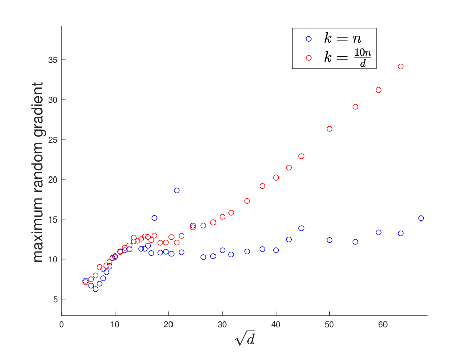
A key fact about generic data, established in Baum 1988; Yun et al. 2019; Bubeck et al. 2020, is that one can memorize arbitrary labels with , that is merely one neuron per datapoints. Our conjecture implies that for such optimal-size neural networks it is impossible to be robust, in the sense that the Lipschitz constant must be of order . The conjecture also states that to be robust (i.e. attain Lipschitz constant ) one must necessarily have , that is roughly each datapoint must have its own neuron. Therefore, we obtain a trade off between size and robustness, namely to make the network robust it needs to be times larger than for mere data fitting. We illustrate these two cases in Figure 1. We train a neural network to fit generic data, and plot the maximum gradient over several randomly drawn points (a proxy for the Lipschitz constant) for various values of , when either (blue dots) or (red dots). As predicted, for the large neural network () the Lipschitz constant remains roughly constant, while for the optimally-sized one () the Lipschitz constant increases roughly linearly in .
Notation.
For we define (if we omit the subscript and write ), where denotes the Euclidean norm. For matrices we use , and for respectively the operator norm, the nuclear norm (sum of singular values), the Frobenius norm, and the Frobenius inner product. We also use these notations for tensors of higher order, see Appendix A for more details on tensors. We denote and for universal numerical constants, respectively small enough and large enough, whose values can change in different occurences. Similarly, by and we denote constants depending only on the parameter . We also write for the rectified linear unit.
Generic data.
We give some flexibility in our definition of “generic data” in order to focus on the essence of the problem, rather than technical details. Namely, in addition to the spherical model mentioned above, where is i.i.d. uniform on the sphere , we also consider the very closely related model where is i.i.d. from a centered Gaussian with covariance (in particular , and in fact is tightly concentrated around ). In both cases we consider to be i.i.d. random signs. We say that a property holds with high probability for generic data, if it holds with high probability either for the spherical model or for the Gaussian model.
2 A conjectured law of robustness
Our main contribution is the following conjecture, which asserts that, on generic data sets, increasing the size of a network is necessary to obtain robustness:
Conjecture 1
For generic data sets, with high probability11 1 We do not quantify the “with high probability” in our conjecture. We believe the conjecture to be true except for an event of exponentially small probability with respect to the sampling of a generic data set, but even proving that the statement is true with strictly positive probability would be extremely interesting., any fitting the data22 2 We expect the same lower bound to hold even if one only asks to approximately fit the data. In fact our provable variants of Conjecture 1 are based proofs that are robust to only assuming an approximately fitting . (i.e., satisfying (2)) must also satisfy:
Note that for generic data, with high probability (for ), there exists a smooth interpolation. Namely there exists with and . This follows easily from the fact that with high probability (for large ) one has . Conjecture 1 puts restrictions on how smoothly one can interpolate data with small neural networks. A striking consequence of the conjecture is that for a two-layers neural network to be as robust as this function (i.e., ) and fit the data, one must have , i.e., roughly one neuron per data point. On the other hand with that many neurons it is quite trivial to smoothly interpolate the data, as we explain in Section 3.3. Thus the conjecture makes a strong statement that essentially the trivial smooth interpolation is the best thing one can do. In addition to making the prediction that one neuron per datapoint is necessary for optimal smoothness, the conjecture also gives a precise prediction on the possible tradeoff between size of the network and its robustness. We also conjecture that this whole range of tradeoffs is actually achievable:
Conjecture 2
Let be such that and where is an arbitrarily large constant in the latter occurence. There exists such that, for generic data sets, with high probability, there exists fitting the data (i.e., satisfying (2)) and such that
The condition in Conjecture 2 is necessary, for any interpolation of the data must have Lipschitz constant at least a constant. The other condition on , namely , is also necessary, for that many neurons is needed to merely guarantee the existence of a data-fitting neural network with neurons (see Baum 1988; Yun et al. 2019; Bubeck et al. 2020). Finally the condition is merely used to avoid explicitly stating a logarithmic term in our conjecture (indeed, equivalently one can replace this condition by adding a multiplicative polylogarithmic term in in the claimed inequality).
Two extreme regimes.
Two regimes of particular interest are the optimal smoothness regime, where we consider how many neurons we need to achieve , and the optimal size regime, where we consider how small a Lipschitz constant is achievable with (i.e., the smallest number of neurons needed to merely fit the data). Our conjectures predict that to be in the optimal smoothness regime it is necessary and sufficient to have , while for optimal size regime it is necessary and sufficient to have .
Our results around Conjecture 2 (Section 3).
We prove Conjecture 2 for both the optimal smoothness regime (which is quite straightforward, see Section 3.3) and for the optimal size regime (here more work is needed, and we use a certain tensor-based construction, see Section 3.4). In the latter case we only prove approximate data fitting (mostly to simplify the proofs), and more importantly we need to assume that is of order for some even integer . It would be interesting to generalize the proof to any . While the conjecture remains open between these two extreme regimes, we do give a construction in Section 3.3 which has the correct qualitative behavior (namely increasing improves the Lipschitz constant), albeit the scaling we obtain is instead of , see Theorem 1.
Our results around Conjecture 1 (Section 4).
We prove a weaker version of Conjecture 1 where the Lipschitz constant on the sphere is replaced by a proxy involving the spectral norm of the weight matrix, see Theorem 3. We also prove the conjecture in the optimal size regime, specifically when for an integer and one uses a polynomial activation function of degree , see Theorem 6. For (i.e., ) we in fact prove the conjecture for abritrary non-linearities, see Theorem 4.
Further open problems.
Our proposed law of robustness is a first mathematical formalization of the broader phenomenon that “overparametrization in neural networks is necessary for robustness”. Ideally one would like a much more refined understanding of the phenomenon than the one given in Conjecture 1. For example, one could imagine that in greater generality, the law would read . That is, we would like to understand how the achievable level of smoothness depends on the particular data set at hand, but also on the set where we expect to be making predictions. Another direction to generalize the law would be to extend it to multi-layers neural networks. In particular one could imagine the most general law would replace the parameter (number of neurons) by the type of architecture being used and in turn predict the best architecture for a given data set and prediction set. Finally note that our proposed law apply to all neural networks, but it would also be interesting to understand how the law interacts with algorithmic considerations (for example in Section 5 we use Adam Kingma and Ba 2015 to find a set of weights that qualitatively match Conjecture 2).
3 Smooth interpolation
We start with a warm-up in Section 3.1 where we discuss the simplest case of interpolation with a linear model () and in Section 3.2 for the optimal smoothness regime (). We generalize the construction of Section 3.2 in Section 3.3 to obtain the whole range of tradeoffs between and , albeit with a suboptimal scaling, see Theorem 1. We also generalize the linear model calculations of Section 3.1 in Section 3.4 to obtain the optimal size regime for larger values of via a certain tensor construction.
3.1 The simplest case: optimal size regime when
Let us consider , and . Thus we are trying to find such that for all , or in other words with the matrix whose row is , and . The smoothest solution to this system (i.e., the one minimizing ) is
Note that
Using [Theorem 5.58, Vershynin 2012] one has with probability at least (and using that ) that
and thus . This concludes the proof sketch of Conjecture 2 for the simplest case and .
3.2 Another simple case: optimal smoothness regime
Next we consider the optimal smoothness regime in Conjecture 2, namely . First note that, for generic data and , with high probability the caps are disjoint sets and moreover they each contain a single data point (namely ). With a single ReLU unit it is then easy to make a smooth function (-Lipschitz) which is outside of and equal to at (in other words the neuron activates for a single data point), namely . Thus one can fit the entire data set with the following ReLU network which is -Lipschitz on the sphere:
This concludes the proof of Conjecture 2 for the optimal smoothness regime .
3.3 Intermediate regimes via ReLU networks
We now combine the two constructions above (the linear model of Section 3.1 and the “isolation” strategy of Section 3.2) to give a construction that can trade off size for robustness (albeit not optimally according to Conjecture 2):
Theorem 1
Let be such that . For generic data sets, with probability at least , there exists fitting the data (i.e., satisfying (2)) and such that
Proof. Let (by assumption ) and assume it is an integer. Let us choose points with the same label, say it is the points with label . As in Section 3.1 let be the minimal norm vector that satisfy , and thus as we proved there with probability at least one has . Crucially for the end of the proof, also note that the distribution of is rotationally invariant. Next observe that with probability at least (with respect to the sampling of ) one has . In particular the cap contains but does not contain any , . Thus the neuron
computes the value at points and the value at the rest of the training set.
One can now repeat this process, and build the neurons (all with norm ), so that (with well-chosen signs ) the data is perfectly fitted by the function:
It only remains to estimate the Lipschitz constant. Note that if a point activates a certain subset of the neurons, then the gradient at this point is with . Using that the are rotationally invariant, one also has with probability at least that for all . Thus it only remains to control how large can be. We show below that with probability at least which will conclude the proof.
If activates neuron then . Now note that for any fixed and fixed , , so that
In particular we conclude that with the probability that a fixed point on the sphere activates more than neuron is exponentially small in (recall that by assumption). Thus we can conclude via an union bound on an -net that the same holds for the entire sphere simultaneously. This concludes the proof.
3.4 Optimal size networks via tensor interpolation
In this section we essentially prove Conjecture 2 in the optimal size regime (namely ), with three caveats:
- 1.
We allow a slack of a factor by considering instead of the optimal as in Baum 1988; Bubeck et al. 2020.
- 2.
We only prove approximate fit rather than exact fit. It is likely that with more work one can use the core of our argument to obtain exact fit. For that reason we did not make any attempt to optimize the dependency on in Theorem 2. For instance one could probably obtain rather than dependency by using an iterative scheme that fits the residuals, as in (Bresler and Nagaraj 2020; Bubeck et al. 2020).
- 3.
Finally we have to assume that is of order for some even integer . While it might be that one can apply the same proof for odd integers, the whole construction crucially relies on being an even integer as we essentially do a linear regression over the feature embedding . A possible approach to extend the proof to other values of would be to use the scheme of Section 3.3 with the linear regression there replaced by the tensor regression of the present section.
Theorem 2
Fix , an even integer, and let . Let be such that and . Then for generic data, with probability at least , there exists such that
| (3) |
and
Proof. We propose to approximately fit with the following neural network:
Naively one might think that this neural network requires neurons. However, it turns out that one can always decompose a symmetric tensor of order into rank- symmetric tensors of order , so that in fact . For this simply follows from eigendecomposition and for general we give a simple proof in [Appendix A, Lemma 2].
4 Provable weaker versions of Conjecture 1
Conjecture 1 can be made weaker along several directions. For example the quantity of interest can be replaced by various upper bound proxies for the Lipschitz constant. A mild weakening would be to replace it by the Lipschitz constant on the whole space (we shall in fact only consider this notion here). A much more severe weakening is to replace it by a quantity that depends on the spectral norm of the weight matrix (essentially ignoring the pattern of activation functions). For the latter proxy we actually give a complete proof, see Theorem 3, which in particular formally proves that “overparametrization is a law of robustness for generic data sets”. Other interesting directions to weaken the conjecture include specializing it to common activation functions, or simply having a smaller lower bound on the Lipschitz constant. In Section 4.2 we prove the conjecture when is replaced by in the lower bound. We say that this inequality is in the “very high-dimensional case”, in the sense that it matches the conjecture for (alternatively we also refer to it as the “undercomplete case”, in the sense that only is relevant in this very high-dimensional scenario). In the moderately high-dimensional case () the proof strategy we propose in Section 4.2 cannot work. In Section 4.3 we give another argument for the latter case, specifically in the optimal size regime (i.e., ) and for a power activation function, see Theorem 5. We generalize this to polynomial activation functions in Section 4.4. In the specific case of a quadratic activation function we also show a lower bound that applies for any and which is in fact larger than the one given in Conjecture 1, see Theorem 7 in Section 4.5.
4.1 Spectral norm proxy for the Lipschitz constant
We can rewrite (1) as
| (4) |
where , , is the matrix whose row is , and is extended from to by applying it coordinate-wise. We prove here the following:
Theorem 3
Assume that is -Lipschitz. For one has
| (5) |
For a generic data set, if and has no bias terms (i.e., in (4)), then with positive probability one has:
| (6) |
Note that we prove the inequality (6) only with positive probability (i.e., there exists a data set where the inequality is true), but in fact it is easy to derive the statement with high probability using classical concentration inequalities.
Next, following the proof of [Proposition 1, Bubeck et al. 2020] one obtains that for a generic data set, with positive probability, one has (without bias terms):
It only remains to observe that:
which concludes the proof of (6).
4.2 Undercomplete case
Next we prove the conjecture in the high dimensional case . More precisely we replace by in the conjectured lower bound. Importantly note that the resulting lower bound then becomes non-trivial only in the regime (the “undercomplete case”).
We consider in fact a slightly more general scenario than interpolation with a neural network, namely we simply assume that one interpolates the data with a function where is a linear projection on a -dimensional subspace (this clearly generalizes , in fact it even allows for the non-linearity to depend on the data33 3 It would be interesting to study whether allowing data-dependent non-linearities could affect the conclusion of our conjectures. Such study would need to crucially rely on having only one hidden layer, as it is known from the Kolmogorov-Arnold theorem that with two hidden layers and data-dependent non-linearities one can obtain perfect approximation properties with (albeit the non-linearities are non-smooth)., or to have a different non-linearity for each neuron).
Theorem 4
Let . Let be a function such that and moreover for some differentiable function and matrix . Then, for generic data, with probability at least one must have
Proof. Let us modify so that is simply an orthogonal projection operator (i.e., ). Let us also assume for sake of notational simplicity that we have a balanced data set of size , that is with: and . Let us denote for . The sequence is i.i.d. and satisfies .
Now observe that on the segment (whose length is less than ), the function changes value from to , and thus there exists such that:
Moreover one has (using that , and thus )
Combining the two above displays one has:
Using [Theorem 5.39, Vershynin 2012] (specifically (5.23)) we know that with probability at least we have (here we use too). Moreover we have . Thus we have so that with the above display one obtains:
which concludes the proof.
4.3 Power activation
We prove here the conjecture for the power activation function with an integer and with no bias terms (we deal with general polynomials, including with bias, in the next section). Without bias such a network can be written as:
| (7) |
where . As we already saw in the proof of Theorem 2 (see specifically [Appendix A, Lemma 2]), without loss of generality we have . We now prove that tensor networks of the form (7) cannot obtain a Lipschitz constant44 4 Note that without loss of generality one can assume to be symmetric, since we only consider how it acts on . For symmetric tensors one has that the Lipschitz constant on the unit ball is lower bounded by the operator norm of thanks to (9) better than , in accordance with Conjecture 1 for full rank tensors (where ).
Theorem 5
Assume that we have a tensor of order such that
Then, for generic data, with probability at least , one must have
4.4 Polynomial activation
We now observe that one can generalize Theorem 5 to handle biases, and in fact even general polynomial activation function. Indeed, observe that any polynomial of must also be a polynomial in , albeit with different coefficients.
Theorem 6
Let and assume that we have such that . Then, for generic data, with probability at least one must have
Proof. Note that for there exists tensors , such that is a tensor of order , and can be written as:
Now let us define , and observe that
and thus there exists such that (we ignore the term by considering the largest balanced subset of the data, i.e. we assume ). Now one can repeat the proof of Theorem 5 to obtain that with probability at least , one has . It only remains to observe that the Lipschitz constant of on the unit ball is lower bounded by .
4.5 Quadratic activation
In Section 4.3 we obtained a lower bound for tensor networks that match Conjecture 1 only when the rank of the corresponding tensor is maximal. Here we show that for quadratic networks (i.e., ) we can match Conjecture 1, and in fact even obtain a better bound, for any rank :
Theorem 7
Assume that we have a matrix with rank such that:
Then, for generic data, with probability at least , one must have
5 Experiments
We consider a generic dataset from the Gaussian model (i.e., i.i.d. from and labels i.i.d from the uniform distribution over and independent of ). For various values of we train two-layers neural networks with units and batch normalization (see Ioffe and Szegedy 2015) between the linear layer and layer, using the Adam optimizer (Kingma and Ba 2015) on the least squares loss. We keep the values of where the network successfully memorizes the random labels (possibly after a rounding to , and such that prior to rounding the least squares loss is at most some small value to be specified later). Given a triple , suppose the output of the trained network is . We then generate (where ) i.i.d from the distribution , independently of everything else and define the “maximum random gradient” to be (it is our proxy for the true Lipschitz constant ). Our experimental results are as follows:
Experiment 1:
We ran experiments with between and , between and , and between and (we also choose for the thresholding). In Figure 3 we give a scatter plot of , and as predicted we see a linear trend, thus providing empirical evidence for Conjecture 1.


Experiment 2:
In this experiment, we investigate the two extreme cases and . We fix and sweep the value of between to (we also choose for the thresholding). In the first case, we let and in the second case we let . In Figure 3 we plot versus the maximum random gradient (as defined above) for both cases. We observe a linear dependence between the maximum gradient value and when we have , and roughly a constant maximum gradient value when , thus providing again evidence for Conjecture 1
References
- Alexander and Hirschowitz [1995] James Alexander and André Hirschowitz. Polynomial interpolation in several variables. Journal of Algebraic Geometry, 4(2):201–222, 1995.
- Allen-Zhu and Li [2020] Zeyuan Allen-Zhu and Yuanzhi Li. Feature purification: How adversarial training performs robust deep learning. arXiv preprint arXiv:2005.10190, 2020.
- Baum [1988] Eric B Baum. On the capabilities of multilayer perceptrons. Journal of complexity, 4(3):193–215, 1988.
- Bresler and Nagaraj [2020] Guy Bresler and Dheeraj Nagaraj. A corrective view of neural networks: Representation, memorization and learning. arXiv preprint arXiv:2002.00274, 2020.
- Bubeck et al. [2019] Sébastien Bubeck, Yin Tat Lee, Eric Price, and Ilya Razenshteyn. Adversarial examples from computational constraints. In International Conference on Machine Learning, pages 831–840, 2019.
- Bubeck et al. [2020] Sébastien Bubeck, Ronen Eldan, Yin Tat Lee, and Dan Mikulincer. Network size and weights size for memorization with two-layers neural networks. arXiv preprint arXiv:2006.02855, 2020.
- Comon et al. [2008] Pierre Comon, Gene Golub, Lek-Heng Lim, and Bernard Mourrain. Symmetric tensors and symmetric tensor rank. SIAM Journal on Matrix Analysis and Applications, 30(3):1254–1279, 2008.
- Cybenko [1989] George Cybenko. Approximation by superpositions of a sigmoidal function. Mathematics of control, signals and systems, 2(4):303–314, 1989.
- Degwekar et al. [2019] Akshay Degwekar, Preetum Nakkiran, and Vinod Vaikuntanathan. Computational limitations in robust classification and win-win results. volume 99 of Proceedings of Machine Learning Research (COLT), pages 994–1028, 2019.
- Friedland and Lim [2018] Shmuel Friedland and Lek-Heng Lim. Nuclear norm of higher-order tensors. Mathematics of Computation, 87(311):1255–1281, 2018.
- Goodfellow et al. [2015] Ian Goodfellow, Jonathon Shlens, and Christian Szegedy. Explaining and harnessing adversarial examples. In International Conference on Learning Representations, 2015.
- Ioffe and Szegedy [2015] Sergey Ioffe and Christian Szegedy. Batch normalization: Accelerating deep network training by reducing internal covariate shift. In International Conference on Machine Learning, pages 448–456, 2015.
- Kingma and Ba [2015] Diederik P Kingma and Jimmy Ba. Adam: A method for stochastic optimization. In International Conference on Learning Representations, 2015.
- Leshno et al. [1993] Moshe Leshno, Vladimir Ya Lin, Allan Pinkus, and Shimon Schocken. Multilayer feedforward networks with a nonpolynomial activation function can approximate any function. Neural networks, 6(6):861–867, 1993.
- Li et al. [2018] Zhening Li, Yuji Nakatsukasa, Tasuku Soma, and André Uschmajew. On orthogonal tensors and best rank-one approximation ratio. SIAM Journal on Matrix Analysis and Applications, 39(1):400–425, 2018.
- Madry et al. [2018] Aleksander Madry, Aleksandar Makelov, Ludwig Schmidt, Dimitris Tsipras, and Adrian Vladu. Towards deep learning models resistant to adversarial attacks. In International Conference on Learning Representations, 2018.
- Nemirovski [2004] Arkadi Nemirovski. Interior point polynomial time methods in convex programming. Lecture notes, 2004.
- Paouris et al. [2017] Grigoris Paouris, Petros Valettas, and Joel Zinn. Random version of dvoretzky’s theorem in lpn. Stochastic Processes and their Applications, 127(10):3187–3227, 2017.
- Raghunathan et al. [2019] Aditi Raghunathan, Sang Michael Xie, Fanny Yang, John C Duchi, and Percy Liang. Adversarial training can hurt generalization. In International Conference on Learning Representations, 2019.
- Reznick [1992] Bruce Arie Reznick. Sum of even powers of real linear forms, volume 463. American Mathematical Soc., 1992.
- Schmidt et al. [2018] Ludwig Schmidt, Shibani Santurkar, Dimitris Tsipras, Kunal Talwar, and Aleksander Madry. Adversarially robust generalization requires more data. In Advances in Neural Information Processing Systems, 2018.
- Szegedy et al. [2013] Christian Szegedy, Wojciech Zaremba, Ilya Sutskever, Joan Bruna, Dumitru Erhan, Ian Goodfellow, and Rob Fergus. Intriguing properties of neural networks. In International Conference on Learning Representations, 2013.
- Vershynin [2012] Roman Vershynin. Introduction to the non-asymptotic analysis of random matrices. In Compressed Sensing: Theory and Practice, pages 210–268. Cambridge University Prteess, 2012.
- Yun et al. [2019] Chulhee Yun, Suvrit Sra, and Ali Jadbabaie. Small relu networks are powerful memorizers: a tight analysis of memorization capacity. In Advances in Neural Information Processing Systems, pages 15532–15543, 2019.
Appendix A Results on tensors
A tensor of order is an array . The Frobenius inner product for tensors is defined by:
with the corresponding norm . A tensor is said to be of rank if it can be written as:
for some . The operator norm is defined by:
For symmetric tensors (i.e., such that the entries of the array are invariant under permutation of the indices), Banach’s Theorem (see e.g., [(2.32), Nemirovski 2004]) states that in fact one has
| (9) |
We refer to Friedland and Lim 2018 for more details and background on tensors. We now list a couple of useful results, with short proofs.
Lemma 1
For a tensor of order , one has
Proof. One has for any ,
Lemma 2
For any tensor of order , there exists and such that for all ,
Results like Lemma 2 go back at least to Reznick 1992. In fact much more precise results on minimal decomposition in rank- tensors are known thanks to the work of Alexander and Hirschowitz 1995. We refer to [Comon et al. 2008] for more discussion on this topic.
Proof. First note that trivially can be written as:
| (10) |
Thus one only needs to prove that a function of the form can be written as the sum of functions of the form . To do so note that, with i.i.d. random signs,
Lemma 3
For any tensor of order one has:
The above result and its proof are directly taken from Li et al. 2018. We only repeat the argument here for sake of completeness.
Proof. Note that the decomposition (10) is orthogonal, and thus for any tensor of order one has:
Thus one has . By duality one also has , which concludes the proof.
Appendix B Results on random tensors
Lemma 4
For any fixed and generic data, with probability at least one has:
Proof. Using [Theorem 1, Paouris et al. 2017] one has, for any fixed and ,
where denotes the moment of the standard Gaussian. Let us denote and , and similarly for . Now with probability (with respect to the randomness of the ) we have
Thus combining the two above displays we obtain with probability at least ,
Lemma 5
For generic data, with probability at least one has:
Proof. Let be an -net of (in particular ). By an union bound and Lemma 4 one has:
| (11) |