Lip-reading with Densely Connected Temporal Convolutional Networks
Abstract
00footnotetext: * Equal Contribution. 00footnotetext: † Corresponding author. 00footnotetext: An improved code implementation is available at: https://github.com/mpc001/Lipreading_using_Temporal_Convolutional_NetworksIn this work, we present the Densely Connected Temporal Convolutional Network (DC-TCN) for lip-reading of isolated words. Although Temporal Convolutional Networks (TCN) have recently demonstrated great potential in many vision tasks, its receptive fields are not dense enough to model the complex temporal dynamics in lip-reading scenarios. To address this problem, we introduce dense connections into the network to capture more robust temporal features. Moreover, our approach utilises the Squeeze-and-Excitation block, a light-weight attention mechanism, to further enhance the model’s classification power. Without bells and whistles, our DC-TCN method has achieved 88.36 % accuracy on the Lip Reading in the Wild (LRW) dataset and 43.65 % on the LRW-1000 dataset, which has surpassed all the baseline methods and is the new state-of-the-art on both datasets.
1 Introduction
Visual Speech Recognition, also known as lip-reading, consists of the task of recognising a speaker’s speech content from visual information alone, typically the movement of the lips. Lip-reading can be extremely useful under scenarios where the audio data is unavailable, and it has a broad range of applications such as in silent speech control system [42], for speech recognition with simultaneous multi-speakers and to aid people with hearing impairment. In addition, lip-reading can also be combined with an acoustic recogniser to improve its accuracy.
Despite of many recent advances, lip-reading is still a challenging task. Traditional methods usually follow a two-step approach. The first stage is to apply a feature extractor such as Discrete Cosine Transform (DCT) [18, 36, 37] to the mouth region of interest (RoI), and then feed the extracted features into a sequential model (usually a Hidden Markov Model or HMM in short) [14, 38, 13] to capture the temporal dynamics. Readers are referred to [57] for more details about these older methods.
The rise of deep learning has led to significant improvement in the performance of lip-reading methods. Similar to traditional approaches, the deep-learning-based methods usually consist of a feature extractor (front-end) and a sequential model (back-end). Autoencoder models were applied as the front-end in the works of [15, 27, 30] to extract deep bottleneck features (DBF) which are more discriminative than DCT features. Recently, the 3D-CNN (typically a 3D convolutional layer followed by a deep 2D Convolutional Network) has gradually become a popular front-end choice [41, 26, 31, 49]. As for the back-end models, Long-Short Term Memory (LSTM) networks were applied in [30, 41, 34, 34] to capture both global and local temporal information. Other widely-used back-end models includes the attention mechanisms [10, 32], self-attention modules [1], and Temporal Convolutional Networks (TCN) [5, 26].
Unlike Recurrent Neural Networks (RNN) such as LSTMs or Gated Recurrent Units (GRUs) [9] with recurrent structures and gated mechanisms, Temporal Convolutional Networks (TCN) adopt fully convolutional architectures and have the advantage of faster converging speed with longer temporal memory. The authors of [5] described a simple yet effective TCN architecture which outperformed baseline RNN methods, suggesting that TCN can be a reasonable alternative for RNNs on sequence modelling problems. Following this work, it was further demonstrated in [26] that a multi-scale TCN could achieve better performance than RNNs on lip-reading of isolated words, which is also the state-of-the-art model so far. Such multi-scale TCN stacks the outputs from convolutions with multiple kernel sizes to gain a more robust temporal features, which has already been shown to be effective in other computer vision tasks utilising multi-scale information such as the semantic segmentation [6, 55, 7]. The TCN architectures in both works [5, 26] have adopted dilated convolutions [53] to enlarge the receptive fields of models. Under the scenarios of lip-reading, a video sequence usually contains various subtle syllables that are essential to distinguish the word or sentence, and thus the model’s abilities to compactly cover those syllables are necessary and important. However, TCN architectures in [5, 26] have utilised a sparse connection and thus may not observe the temporal features thoroughly and densely.
Inspired by recent success of Densely Connected Networks [20, 51, 16], we introduce dense connections into the TCN structures and propose the Densely Connected TCN (DC-TCN) for word-level lip-reading. DC-TCNs are able to cover the temporal scales in a denser fashion and thus are more sensitive to words that may be challenging to previous TCN architectures [5, 26]. Specifically, we explore two approaches of adding dense connections in the paper. One is a fully dense (FD) TCN model, where the input of each Temporal Convolutional (TC) layers is the concatenations of feature maps from all preceding TC layers. Another DC-TCN variant employs a partially dense (PD) structures. We further utilise the Squeeze-and-Excitation (SE) attention machanism[19] in both DC-TCN variants, which further enhances their classification power.
To validate the effectiveness of the proposed DC-TCN models, we have conducted experiments on the Lip Reading in the Wild (LRW) [11] dataset and LRW-1000 dataset [52], which are the largest publicly available benchmark datasets for unconstrained lip-reading in English and in Mandarin, respectively. Our final model achieves 88.36 % accuracy on LRW, surpassing the current state-of-the-art method [26] (85.3 %) by around 3.1 %. On LRW-1000, our method gains 43.65 % accuracy and also out-perform all baselines, demonstrating the generality and strength of the proposed DC-TCN.
In general, this paper presents the following contributions :
1. We propose a Densely Connected Temporal Convolutional Network (DC-TCN) for lip-reading of isolated words, which can provide denser and more robust temporal features.
2. Two DC-TCN variants with Squeeze-and-excitation blocks [19], namely the fully dense (FD) and partially dense (PD) architectures, are introduced and evaluated in this paper.
3. Our method has achieved 88.36 % top-1 accuracy on LRW dataset and 43.65 % and on LRW-1000, which have surpassed all baseline methods and set a new record on these two datasets.
2 Related Works
2.1 Lip-reading
Early deep learning methods for lip-reading of isolated words were mainly evaluated on small-scale datasets recorded in constrained environments such as OuluVS2 [2] and CUAVE [29]. The authors of [30] proposed to use the combination of deep bottleneck features (DBF) and DCT features to train a LSTM classifier, which is not end-to-end trainable. An end-to-end trainable model was first demonstrated in [46] using Histogram of Oriented Gradient (HOG) features with LSTMs, and later Petridis et al. [34] trained an end-to-end model with a Bidirectional LSTM back-end where the first and second derivatives of temporal features are also computed, achieving much better results than [46]. The lip-reading accuracy on those small-scale datasets are further improvded by the introduction of multi-view visual information [34] and audio-visual fusion [33, 35].
Lip Reading in the Wild (LRW) dataset [11] is the first and the largest publicly available dataset for unconstrained lip-reading with a 500-word English vocabulary. It has encouraged the emergence of numerous deep learning models with more and more powerful word-recognising abilities. The WLAS sequence-to-sequence model [10] consists of a VGG network [39] and a LSTM with dual attention systems on visual and audio stream, respectively. LipNet [3] is the first approach to employ a 3D-CNN to extract spatial-temporal features that are classified by Bidirectional Gated Recurrent Units (BGRUs). A 2D Residual Network (ResNet) [17] on top of a 3D Convolutional layer is used as the front-end in [41] (with an LSTM as the back-end). Two 3D ResNets are organised in a two-stream fashion (one stream for image and another for optical flow) in the work of [49], learning more robust spatial-temporal features at the cost of larger network size. Cheng et al. [8] propose a technique of pose augmentation to enhance the performance of lip-reading in extreme poses. Zhang et al. [54] propose to incorporate other facial parts in additional to the mouth region to solve lip-reading of isolated words, and mutual information constrains are added in [56] to produce more discriminative features. The current state-of-the-art performance on LRW is achieved by [26], which has replaced RNN back-ends with a multi-scale Temporal Convolutional Networks (TCN). The same model achieves the state-of-the-art performance on LRW-1000 [52] dataset which is currently the largest lip-reading dataset for Mandarin.
2.2 Temporal convolutional networks
Although RNN networks such as LTSMs or GRUs had been commonly used in lip-reading methods to model the temporal dependencies, alternative light-weight, faster-converging CNN models have started to gain attention in recent works. Such efforts can be traced back to the Time-Delay Neural Networks (TDNN) [45] in 1980s. Consequently, models with Temporal Convolutions were developed, including WaveNet [43] and Gated ConNets [12]. Lately, Bai et al. [5] described a simple and generic Temporal Convolutional Network (TCN) architecture that out-performed baseline RNN models in various sequence modelling problems. Although the TCN introduced in [5] is a causal one in which no future features beyond the current time step can be seen in order to prevent the leakage of future information, the model can also be modified into a non-causal variant without such constrains. The work of [26] has adopted a non-casual TCN design, where the linear TC block architecture was replaced with a multi-scale one. To the best of our knowledge, this work [26] has achieved the current state-of-the-art performance on the LRW dataset. However, the receptive field scales in such TCN architectures may not be able cover the full temporal range under lip-reading scenarios, which can be solved by the employment of dense connections.
2.3 Densely connected networks
Densely connected network has received broad attention since its inception in [20], where a convolutional layer receives inputs from all its preceding layers. Such densely connected structure can effectively solve the vanishing-gradient problem by employing shallower layers and thus benefiting feature propagation. The authors of [51] have applied dense connections to dilated convolutions to enlarge the receptive field sizes and to extract denser feature pyramid for semantic segmentation. Recently, a simple dense TCN for Sign Language Translation has been illustrated in [16]. Our work is the first to explore the densely connected TCN for for word-level lip-reading, where we present both a fully dense (FD) and a partially dense (PD) block architectures with the addition of the channel-wise attention method described in [19].
2.4 Attention and SE blocks
Attention mechanism [4, 25, 44, 48] can be used to teach the network to focus on the more informative locations of input features. In lip-reading, attention mechanisms have been mainly developed for sequence models like LSTMs or GRUs. A dual attention mechanism is proposed in [10] for the visual and audio input signals of the LSTM models. Petridis et al. [32] have coupled the self-attention [44] block with a CTC loss to improve the performance of Bidirectional LSTM classifiers. Those attention methods are somehow computational expensive and are inefficient to be integrated into TCN structures. In this paper, we adopt a light-weight attention block, which is the Squeeze-and-Excitation (SE) network [19], to introduce the channel-wise attention into the DC-TCN network.
In particular, denote the input tensor of a SE block as where is the channel number, its channel-wise descriptor is first be obtained by a global average pooling operation to squeeze the spatial dimension , i.e. where denotes the global average pooling. After that, an excitation operation is applied to to obtain the channel-wise dependencies , which can be expressed as . Here, and are learnable weights, while and stands for the sigmoid activation and ReLU functions and represents the reduction ratio. The final output of the SE block is simply the channel-wise broadcasting multiplication of and . The readers are referred to [19] for more details.
3 Methodology
3.1 Overview

Fig. 1 depicts the general framework of our method. The input is the cropped gray-scale mouth RoIs with the shape of , where stands for the temporal dimension and , represent the height and width of the mouth RoIs, respectively. Note that we have ignored the batch size for simplicity. Following [41, 26], we first utilise a 3D convolutional layer to obtain the spatial-temporal features with shape , where is the feature channel number. On top of this layer, a 2D ResNet-18 [17] is applied to produce features with shape . The next layer applies the average pooling to summarise the spatial knowledge and to reduce the dimensionality to . After this pooling operation, the proposed Densely Connected TCN (DC-TCN) is employed to model the temporal dynamics. The output tensor () is passed through another average pooling layer to summarise temporal information into channels, while represents the classes to be predicted. The word class probabilities are predicted by the succeeding softmax layer. The whole model is end-to-end trainable.
3.2 Densely Connected TCN


To introduce the proposed Densely Connected TCN (DC-TCN), we start from a brief explanation of the temporal convolution in [5]. A temporal convolution is essentially a 1-D convolution operating on temporal dimensions, while a dilation [53] is usually inserted into the convolutional filter to enlarge the receptive fields. Particularly, for a 1-D feature where is the temporal dimensionality, define a discrete function such that where , let and be a 1D discrete filter of size , a temporal convolution with dilation rate is described as
| (1) |
where is the 1-D output feature and refers to its -th element. Note that zero padding is used to keep the temporal dimensionality unchanged in . Note that the temporal convolution described in Eq. 1 is non-casual, i.e. the filters can observe features of every time step, similarly to that of [26]. Fig. 2 has provided a intuitive example of the non-casual temporal convolution layers.
Let be the -th temporal convolution layer, and let and be its input and output tensors with and channels, respectively, i.e. . In common TCN architectures, is directly fed into the -th temporal convolution layer to produce its output , which is depicted as
| (2) |
In DC-TCN, dense connections [20] are utilised and the input for the following TC layer () is the concatenation between and , which can be written as
| (3) |
Note that has additional channels () than , where is defined as the growth rate following [20].
We have embedded the dense connections in Eq. 3 to constitute the block of DC-TCN. More formally, we define a DC-TCN block to consist of temporal convolution (TC) layers with arbitrary but unique combinations of filter size and dilation rate , where and stand for the sets of all available filter sizes and dilation rates for this block, respectively. For example, if we define a block to have filter sizes set and dilation rates set , there will be four TC layers () in this block.
In this paper, we study two approaches of constructing DC-TCN blocks. The first approach applies dense connections for all TC layers, which is denoted as the fully dense (FD) block, as illustrated at the top of Fig. 3, where the block filter sizes set and the dilation rates set . As shown in the figure, the output tensor of each TC layer is consistently concatenated to the input tensor, increasing the input channels by (the growth rate) each time. Note that we have a Squeeze-and-Excitation (SE) block [19] after the input tensor of each TC layer to introduce channel-wise attentions for better performance. Since the output of the top TC layer in the block typically has much more channels than the block input (e.g. channels in Fig. 3), we employ a 11 convolutional layer to reduce its channel dimensionality from to for efficiency (“Reduce Layer” in Fig. 3). A 11 convolutional layer is then applied to convert the block input’s channels if . In the fully dense architecture, TC layers are stacked in a receptive-field-ascending order.
Another DC-TCN block design is depicted at the bottom of Fig. 3, which we denote as the partially dense (PD) block. In the PD block, filters with identical dilation rates are employed in a multi-scale fashion, such as the and TC layers in Fig. 3 (bottom), and their outputs are concatenated to the input simultaneously. PD block is a essentially a hybrid of the multi-scale architectures and densely connected networks, and thus is expected to benefit from both. Just like in FD architectures, SE attention is also attached after every input tensor, while the ways of utilising the reduce layer is the same to that of fully dense blocks.
A DC-TCN block, either fully or partially dense, can be seamlessly stacked with another block to obtain finer features. A fully dense / partially dense DC-TCN model can be formed by stacking identical FD / PD blocks together, where denotes the number of blocks.
There are various important network parameters to be determined for a DC-TCN model, including the filter sizes and the dilation rates in each block, the growth rate , and the reduce layer channel and the blocks number . The optimal DC-TCN architecture along with the process of determining it can be found in Sec. 4.3.
3.3 Advantages of DC-TCN

The receptive field size for a filter with kernel size and dilation rate can be calculated as
| (4) |
Stacking two TC layers with receptive fields and will produce a receptive field size of . The receptive field sizes for the four TC layers described in Fig. 3 are and , respectively. If they are connected linearly as in [5], the resulting model can see a temporal range of . A multi-scale structure [26] will lead to receptive fields of . The linearly connected architecture retains a larger maximum receptive size than the multi-scale one, however, it also generate more sparse temporal features. We have illustrated the receptive fields for these two block architectures in Fig. 4.
Unlike the linearly connected [5] or multi-scale [26] TCN, our DC-TCN can extract the temporal features at denser scales and thus increase the features’ robustness without reducing the maximum receptive field size. Fig. 5 depicts the temporal range covered by our partially dense and fully dense blocks, which consist of the four identical TC layers as shown in Fig. 4. Since we have introduced dense connection (“DC” in the figure) into the structure, a TC layer can see all the preceding layers and therefore the varieties of its receptive sizes are significantly enhanced. As shown in Fig. 5 (left), our partially dense block can observe a total of eight different ranges, which is double of that in linear or multi-scale architectures (only 4 scales). The fully dense block in Fig. 5 (right) can produce feature pyramid from 15 different receptive fields with the maximum one to be 31 (larger than multi-scale and equal to linear). Such dense receptive fields can ensure that the information from a wide range of scales can be observed by the model, and thus strengthen the model’s expression power.

4 Experiments
4.1 Datasets
We have conducted our experiments on the Lip Reading in the Wild (LRW) [11] and the LRW-1000 [52] dataset, which are the largest publicly available dataset for lipreading of isolated words in English and in Mandarin, respectively.
The LRW dataset has a vocabulary of 500 English words. The sequences in LRW are captured from more than 1 000 speakers in BBC programs, and each sequence has a duration of 1.16 seconds (29 video frames). There are a total of 538 766 sequences in this dataset, which are split into 488 766/25 000/25 000 for training/validation/testing usages. This is a challenging dataset due to the large number of subjects and variations in head poses and lighting conditions.
The LRW-1000 dataset contains a total of 718 018 samples for 1 000 mandarin words, recorded from more than 2 000 subjects. The average duration for each sequence is 0.3 second, and the total length of all sequences is about 57 hours. The training/validation/testing splits consist of 603 193/63 237/51 588 samples, respectively. This dataset is even more challenging than LRW considering its huge variations in speaker properties, background clutters, scale, etc.
4.2 Experimental setup
Pre-processing We have pre-processed the LRW dataset following the same method as described in [26]. We first detect 68 facial landmarks using dlib [22]. Based on the coordinates of these landmarks, the face images are warped to a reference mean face shape. Finally, the mouth RoI of size 9696 is cropped from each warped face image and is converted into grayscale. For LRW-1000, we simply use the provided pre-cropped mouth RoIs and resize them to 122122 following [52].
Evaluation metric Top-1 accuracy is used to evaluate the model performance, since we are solving word-level lip-reading classification problems.
Training settings The whole model in Fig. 1, including the proposed DC-TCN, is trained in an end-to-end fashion, where the weights are randomly initialised. We employ identical training settings for both LRW and LRW-1000 datasets except of some slight differences to cope with their different input dimensions. We train 80 epochs with a batch size of 32/16 on LRW/LRW-1000, respectively, and measure the top-1 accuracy using the validation set to determine the best-performing checkpoint weights. We adopt AdamW [24] as the optimiser, where the initial learning rate is set to 0.0003/0.0015 for LRW and LRW-1000, respectively. A cosine scheduler [23] is used to steadily decrease the learning rate from the initial value to 0. BatchNorm layers [21] are embedded to accelerate training convergence, and we use dropouts with dropping probabilities 0.2 for regularisation. The reduction ratio in the SE block is set to 16, and the channel value of DC-TCN’s input tensor is set to 512. Besides, we adopt the variable length augmentation as proposed in [26] to increase the model’s temporal robustness.
Explorations of DC-TCN structures We evaluate DC-TCN with different structure parameters on LRW dataset to determine the best-performing one. In particular, we first validate the effectiveness of different filter sizes and dilation rates in each DC-TCN block while freezing other hyper-parameters such as the growth rate and the reduce layer channels . Then we select the most effective and values to fine-tune other structural options, including the growth rate and whether to use SE attention. We explore structures for both FD and PD blocks.
Baseline methods On the LRW dataset, the performance of the proposed DC-TCN model is compared with the following baselines: 1) the method proposed in the LRW paper [11] with a VGG backbone [39], 2) the WLAS model [10], 3) the work of [41] where a ResNet [17] and a LSTM is used, 4) the End-to-End Audio-Visual network [31], 5) the multi-grained spatial-temporal model in [47], 6) the two-stream 3D CNN in [49], 7) the Global-Local Mutual Information Maximisation method in [56], 8) the face region cutout approach by authors of [54], 9) the multi-modality speech recognition method in [50], and 10) the multi-scale TCN proposed by [26].
LRW-1000 is a relatively new dataset and there are somehow fewer works on it. We have selected the following methods as baselines on this dataset: 1) the work of [41], 2) the multi-grained spatial-temporal model in [47], 3) the GLMIM method in [56] and 4) the multi-scale TCN [26].
Implementations We implement our method in the PyTorch framework [28]. Experiments are conducted on a server with eight 1080Ti GPUs. It takes around four days to train a single model end-to-end on LRW using one GPU and five days for LRW-1000. Note that this training time is significantly lower than other works [31] which requires approximately three weeks per GPU for a training cycle.
4.3 Results
DC-TCN architectures To find an optimal structure of DC-TCN, we first evaluate the impact of various filter sizes and dilation rates on LRW while keeping the value of other hyper-parameters fixed. In particular, we fix the growth rate and the reduce layer channels to be 64 and 512, respectively, and stack a total of 4 DC-TCN blocks without SE attention. As shown in Table 1, both Fully Dense (FD) and Partially Dense (PD) blocks achieve optimal performance when and are set to be and , respectively. Therefore, we decide to use this setting for and in subsequent experiments.
| Filter Sizes | Dilation Rates | Acc. (%, FD) | Acc. (%, PD) |
| {3,5} | {1,2,3} | 86.68 | 86.84 |
| {3,5,7} | {1,2} | 86.88 | 87.01 |
| {1,2,4} | 87.07 | 87.48 | |
| {1,2,5} | 87.11 | 87.50 | |
| {3,5,7,9} | {1,2} | 86.99 | 87.26 |
| {1,2,4} | 86.92 | 87.15 | |
| {1,2,5} | 86.85 | 87.16 |
| Growth rate | Adding SE | Acc. (%, FD) | Acc. (%, PD) |
|---|---|---|---|
| 64 | - | 87.11 | 87.50 |
| 64 | ✓ | 87.40 | 87.91 |
| 128 | - | 87.64 | 88.13 |
| 128 | ✓ | 88.01 | 88.36 |
Once the optimal values of and are found, we have further investigated the effect of different growth rate settings and the addition of SE block, while the reduce layer channels and the total block number are set to 512 and 4, respectively. As shown in 2, it is evident that: 1. the performance of using 128 for exceeds that of using 64, and 2. the effectiveness of adding SE in the block is validated since it consistently leads to higher accuracy when stays the same.
To sum up, we have selected the following hyper-parameters as the final DC-TCN model configuration for both FD and PD: the filter sizes and dilation rates in each block are set to and , with the growth rate , the reduce layer channel and the block number , where SE attention is added after each input tensor.
| Methods | Front-end | Back-end | Acc. (%) |
| LRW [11] | VGG-M | - | 61.1 |
| WLAS [10] | VGG-M | LSTM | 76.2 |
| ResNet+BLSTM [41] | 3D Conv + ResNet34 | BLSTM | 83.0 |
| End-to-End AVR [31] | 3D Conv + ResNet34 | BLSTM | 83.4 |
| Multi-grained ST [47] | ResNet34 + DenseNet3D | Conv-BLSTM | 83.3 |
| Two-stream 3D CNN [49] | (3D Conv)2 | BLSTM | 84.1 |
| ResNet18 + BLSTM[40] | 3D Conv + ResNet18 | BLSTM | 84.3 |
| GLMIM [56] | 3D Conv + ResNet18 | BGRU | 84.4 |
| Face cutout [54] | 3D Conv + ResNet18 | BGRU | 85.0 |
| Multi-modality SR [50] | 3D ResNet50 | TCN | 84.8 |
| Multi-scale TCN [26] | 3D Conv + ResNet18 | MS-TCN | 85.3 |
| Ours | 3D Conv + ResNet18 | DC-TCN (PD) | 88.36 |
| DC-TCN (FD) | 88.01 |
| Methods | Front-end | Back-end | Acc. (%) |
| ResNet+LSTM [52] | 3D Conv + ResNet34 | LSTM | 38.2 |
| Multi-grained ST [47] | ResNet34 + DenseNet3D | Conv-BLSTM | 36.9 |
| GLMIM [56] | 3D Conv + ResNet18 | BGRU | 38.79 |
| Multi-scale TCN [26] | 3D Conv + ResNet18 | MS-TCN | 41.4 |
| Ours | 3D Conv + ResNet18 | DC-TCN (PD) | 43.65 |
| DC-TCN (FD) | 43.11 |
| Drop Frames | =0 | =1 | =2 | =3 | =4 | =5 |
|---|---|---|---|---|---|---|
| End-to-End AVR [31] 11 1 3D Conv+ResNet18 as front-end and BGRU as back-end. | 84.6 | 80.2 | 71.3 | 59.5 | 45.9 | 32.9 |
| MS-TCN [26] | 85.3 | 83.5 | 81.2 | 78.7 | 75.7 | 71.5 |
| Ours (PD) | 88.4 | 86.2 | 84.0 | 81.0 | 77.5 | 73.3 |
| Ours (FD) | 88.0 | 86.4 | 83.6 | 81.3 | 77.7 | 73.8 |
Performance on the LRW and LRW-1000 datasets In Table 3 and 4 we report the performance of our method and various baseline approaches on the LRW and LRW-1000 datasets, respectively. On LRW, our method has achieved an accuracy of 88.01 % (FD blocks) and 88.36 % (PD blocks), which is the new state-of-the-art performance on this dataset with an absolution improvement of 3.1 % over the current state-of-the-art method [26] on the LRW dataset. Besides, our method also produces higher top-1 accuracy (43.65 % and 43.11 % by using PD and FD, respectively) than the best baseline method [26] (41.4 %) on LRW-1000, which has further validated the generality and effectiveness of the proposed DC-TCN model.
4.4 Discussion
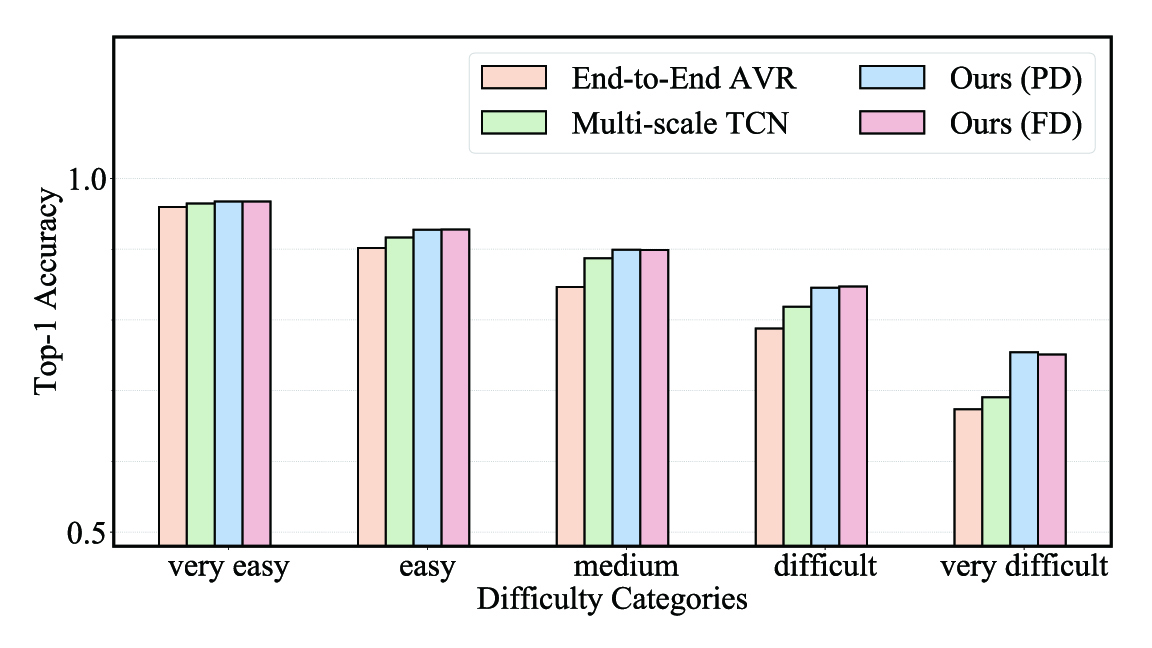
Difficulty Categories To intuitively illustrate why our DC-TCN can out-perform the baseline methods, we have examined the classification rates of different methods on five word categories with various difficulty levels. To be specific, we have divided the 500 classes in the LRW test set into five categories (100 words per category) based on their classification difficulty in [26], which are “very easy”, “easy”, “medium”, “difficult” and “very difficult”. Then we compare the performance of our DC-TCN (FD and PD) with two baseline methods (End-to-End AVR [31] and Multi-scale TCN [26]) on those five difficulty categories, as demonstrated in Fig. 6. We observe that our methods result in slightly better performance than the baselines on the “very easy” and “easy” categories, however, improvements over the baselines are more significant on the other three groups, especially on the “difficult” and the “very difficult” categories. Since the improvement of our methods is mainly achieved on those more difficult words, it is reasonably to deduce that our DC-TCN can extract more robust temporal features.
Variable Lengths We further evaluate the temporal robustness of different models against video sequences with variable lengths, i.e. frames are randomly dropped from each testing sequence in LRW dataset where ranges from 0 to 5. As shown in Table 5, the performance of End-to-End AVR [31] drops significantly as increasing frames are randomly removed from the testing sequences. In contrast, MS-TCN [26] and our DC-TCN (both PD and FD) demonstrate better tolerance to such frame removals, mainly due to the usage of variable length augmentation [26] during training. Besides, the accuracy of our models (both PD and FD) constantly outperforms that of MS-TCN [26] no matter how the number of frames to remove varies, which verifies the superior temporal robustness of our method.
5 Conclusion
We have introduced a Densely Connected Temporal Convolution Network (DC-TCN) for word-level lip-reading in this paper. Characterised by the dense connections and the SE attention mechanism, the proposed DC-TCN can capture more robust features at denser temporal scales and therefore improve the performance of the original TCN architectures. DC-TCN have surpassed the performance of all baseline methods on both the LRW dataset and the LRW-1000 dataset. To the best of our knowledge, this is the first attempt to adopt a densely connected TCN with SE attention for lip-reading of isolated words, resulting in new state-of-the-art performance.
Acknowledgements
The work of Pingchuan Ma has been partially supported by Honda and the “AWS Cloud Credits for Research” program. The work of Yujiang Wang has been partially supported by China Scholarship Council (No. 201708060212) and the EPSRC project EP/N007743/1 (FACER2VM).
References
- [1] Triantafyllos Afouras, Joon Son Chung, Andrew Senior, Oriol Vinyals, and Andrew Zisserman. Deep audio-visual speech recognition. IEEE transactions on pattern analysis and machine intelligence, 2018.
- [2] Iryna Anina, Ziheng Zhou, Guoying Zhao, and Matti Pietikäinen. Ouluvs2: A multi-view audiovisual database for non-rigid mouth motion analysis. In Proceedings of FG, volume 1, pages 1–5, 2015.
- [3] Yannis M. Assael, Brendan Shillingford, Shimon Whiteson, and Nando de Freitas. Lipnet: Sentence-level lipreading. CoRR, abs/1611.01599, 2016.
- [4] Dzmitry Bahdanau, Kyunghyun Cho, and Yoshua Bengio. Neural machine translation by jointly learning to align and translate. In Proceedings of ICLR, 2015.
- [5] Shaojie Bai, J Zico Kolter, and Vladlen Koltun. An empirical evaluation of generic convolutional and recurrent networks for sequence modeling. arXiv preprint arXiv:1803.01271, 2018.
- [6] Liang-Chieh Chen, George Papandreou, Iasonas Kokkinos, Kevin Murphy, and Alan L Yuille. Deeplab: Semantic image segmentation with deep convolutional nets, atrous convolution, and fully connected crfs. IEEE transactions on pattern analysis and machine intelligence, 40(4):834–848, 2017.
- [7] Liang-Chieh Chen, George Papandreou, Florian Schroff, and Hartwig Adam. Rethinking atrous convolution for semantic image segmentation. arXiv preprint arXiv:1706.05587, 2017.
- [8] Shiyang Cheng, Pingchuan Ma, Georgios Tzimiropoulos, Stavros Petridis, Adrian Bulat, Jie Shen, and Maja Pantic. Towards pose-invariant lip-reading. In Proceedings of ICASSP, pages 4357–4361, 2020.
- [9] Kyunghyun Cho, Bart van Merrienboer, Çaglar Gülçehre, Dzmitry Bahdanau, Fethi Bougares, Holger Schwenk, and Yoshua Bengio. Learning phrase representations using RNN encoder-decoder for statistical machine translation. In Proceedings of EMNLP, pages 1724–1734, 2014.
- [10] Joon Son Chung, Andrew Senior, Oriol Vinyals, and Andrew Zisserman. Lip reading sentences in the wild. In Proceedings of CVPR, pages 3444–3453, 2017.
- [11] Joon Son Chung and Andrew Zisserman. Lip reading in the wild. In Proceedings of ACCV, pages 87–103, 2016.
- [12] Yann N. Dauphin, Angela Fan, Michael Auli, and David Grangier. Language modeling with gated convolutional networks. In Proceedings of ICML, volume 70, pages 933–941, 2017.
- [13] Stéphane Dupont and Juergen Luettin. Audio-visual speech modeling for continuous speech recognition. IEEE transactions on multimedia, 2(3):141–151, 2000.
- [14] Virginia Estellers, Mihai Gurban, and Jean-Philippe Thiran. On dynamic stream weighting for audio-visual speech recognition. IEEE Transactions on Audio, Speech, and Language Processing, 20(4):1145–1157, 2011.
- [15] Jonas Gehring, Yajie Miao, Florian Metze, and Alex Waibel. Extracting deep bottleneck features using stacked auto-encoders. In Proceedings of ICASSP, pages 3377–3381, 2013.
- [16] Dan Guo, Shuo Wang, Qi Tian, and Meng Wang. Dense temporal convolution network for sign language translation. In Proceedings of IJCAI, pages 744–750, 2019.
- [17] K. He, X. Zhang, S. Ren, and J. Sun. Deep residual learning for image recognition. In Proceedings of CVPR, pages 770–778, 2016.
- [18] Xiaopeng Hong, Hongxun Yao, Yuqi Wan, and Rong Chen. A pca based visual dct feature extraction method for lip-reading. In 2006 International Conference on Intelligent Information Hiding and Multimedia, pages 321–326, 2006.
- [19] Jie Hu, Li Shen, and Gang Sun. Squeeze-and-excitation networks. In Proceedings of CVPR, pages 7132–7141, 2018.
- [20] Gao Huang, Zhuang Liu, Laurens Van Der Maaten, and Kilian Q Weinberger. Densely connected convolutional networks. In Proceedings of CVPR, pages 4700–4708, 2017.
- [21] Sergey Ioffe and Christian Szegedy. Batch normalization: Accelerating deep network training by reducing internal covariate shift. In Proceedings of ICML, volume 37, pages 448–456, 2015.
- [22] Davis E King. Dlib-ml: A machine learning toolkit. Journal of Machine Learning Research, 2009.
- [23] Ilya Loshchilov and Frank Hutter. SGDR: stochastic gradient descent with warm restarts. In Proceedings of ICLR, 2017.
- [24] Ilya Loshchilov and Frank Hutter. Decoupled weight decay regularization. In Proceedings of ICLR, 2019.
- [25] Thang Luong, Hieu Pham, and Christopher D. Manning. Effective approaches to attention-based neural machine translation. In Proceedings of EMNLP, pages 1412–1421, 2015.
- [26] Brais Martinez, Pingchuan Ma, Stavros Petridis, and Maja Pantic. Lipreading using temporal convolutional networks. Proceedings of ICASSP, pages 6319–6323, 2020.
- [27] Kuniaki Noda, Yuki Yamaguchi, Kazuhiro Nakadai, Hiroshi G Okuno, and Tetsuya Ogata. Audio-visual speech recognition using deep learning. Applied Intelligence, 42(4):722–737, 2015.
- [28] Adam Paszke, Sam Gross, Francisco Massa, Adam Lerer, James Bradbury, Gregory Chanan, Trevor Killeen, Zeming Lin, Natalia Gimelshein, Luca Antiga, et al. Pytorch: An imperative style, high-performance deep learning library. In Proceedings of NIPS, pages 8026–8037, 2019.
- [29] Eric K. Patterson, Sabri Gurbuz, Zekeriya Tufekci, and John N. Gowdy. Moving-talker, speaker-independent feature study, and baseline results using the CUAVE multimodal speech corpus. EURASIP J. Adv. Signal Process., 2002(11):1189–1201, 2002.
- [30] Stavros Petridis and Maja Pantic. Deep complementary bottleneck features for visual speech recognition. In Proceedings of ICASSP, pages 2304–2308, 2016.
- [31] Stavros Petridis, Themos Stafylakis, Pingehuan Ma, Feipeng Cai, Georgios Tzimiropoulos, and Maja Pantic. End-to-end audiovisual speech recognition. In Proceedings of ICASSP, pages 6548–6552, 2018.
- [32] Stavros Petridis, Themos Stafylakis, Pingchuan Ma, Georgios Tzimiropoulos, and Maja Pantic. Audio-visual speech recognition with a hybrid ctc/attention architecture. In Proceedings of SLT, pages 513–520, 2018.
- [33] Stavros Petridis, Yujiang Wang, Zuwei Li, and Maja Pantic. End-to-end audiovisual fusion with lstms. In Proceedings of AVSP, pages 36–40, 2017.
- [34] Stavros Petridis, Yujiang Wang, Zuwei Li, and Maja Pantic. End-to-end multi-view lipreading. In Proceedings of BMVC, 2017.
- [35] Stavros Petridis, Yujiang Wang, Pingchuan Ma, Zuwei Li, and Maja Pantic. End-to-end visual speech recognition for small-scale datasets. Pattern Recognition Letters, 131:421–427, 2020.
- [36] Gerasimos Potamianos, Chalapathy Neti, Guillaume Gravier, Ashutosh Garg, and Andrew W Senior. Recent advances in the automatic recognition of audiovisual speech. Proceedings of the IEEE, 91(9):1306–1326, 2003.
- [37] Gerasimos Potamianos, Chalapathy Neti, Giridharan Iyengar, Andrew W Senior, and Ashish Verma. A cascade visual front end for speaker independent automatic speechreading. International Journal of Speech Technology, 4(3-4):193–208, 2001.
- [38] Xu Shao and Jon Barker. Stream weight estimation for multistream audio–visual speech recognition in a multispeaker environment. Speech Communication, 50(4):337–353, 2008.
- [39] Karen Simonyan and Andrew Zisserman. Very deep convolutional networks for large-scale image recognition. In Proceedings of ICLR, 2015.
- [40] Themos Stafylakis, Muhammad Haris Khan, and Georgios Tzimiropoulos. Pushing the boundaries of audiovisual word recognition using residual networks and LSTMs. Computer Vision and Image Understanding, 176–177:22–32, 2018.
- [41] Themos Stafylakis and Georgios Tzimiropoulos. Combining residual networks with lstms for lipreading. In Proceedings of Interspeech, pages 3652–3656, 2017.
- [42] Ke Sun, Chun Yu, Weinan Shi, Lan Liu, and Yuanchun Shi. Lip-interact: Improving mobile device interaction with silent speech commands. In Proceedings of the 31st Annual ACM Symposium on User Interface Software and Technology, pages 581–593, 2018.
- [43] Aäron van den Oord, Sander Dieleman, Heiga Zen, Karen Simonyan, Oriol Vinyals, Alex Graves, Nal Kalchbrenner, Andrew W. Senior, and Koray Kavukcuoglu. Wavenet: A generative model for raw audio. In ISCA Speech Synthesis Workshop, page 125, 2016.
- [44] Ashish Vaswani, Noam Shazeer, Niki Parmar, Jakob Uszkoreit, Llion Jones, Aidan N. Gomez, Lukasz Kaiser, and Illia Polosukhin. Attention is all you need. In Proceedings of NIPS, pages 5998–6008, 2017.
- [45] Alex Waibel, Toshiyuki Hanazawa, Geoffrey Hinton, Kiyohiro Shikano, and Kevin J Lang. Phoneme recognition using time-delay neural networks. volume 37, pages 328–339, 1989.
- [46] Michael Wand, Jan Koutník, and Jürgen Schmidhuber. Lipreading with long short-term memory. In Proceedings of ICASSP, pages 6115–6119, 2016.
- [47] Chenhao Wang. Multi-grained spatio-temporal modeling for lip-reading. In Proceedings of BMVC, page 276, 2019.
- [48] Xiaolong Wang, Ross Girshick, Abhinav Gupta, and Kaiming He. Non-local neural networks. In Proceedings of CVPR, pages 7794–7803, 2018.
- [49] Xinshuo Weng and Kris Kitani. Learning spatio-temporal features with two-stream deep 3d cnns for lipreading. In Proceedings of BMVC, page 269, 2019.
- [50] Bo Xu, Cheng Lu, Yandong Guo, and Jacob Wang. Discriminative multi-modality speech recognition. In Proceedings of CVPR, 2020.
- [51] Maoke Yang, Kun Yu, Chi Zhang, Zhiwei Li, and Kuiyuan Yang. Denseaspp for semantic segmentation in street scenes. In Proceedings of CVPR, pages 3684–3692, 2018.
- [52] Shuang Yang, Yuanhang Zhang, Dalu Feng, Mingmin Yang, Chenhao Wang, Jingyun Xiao, Keyu Long, Shiguang Shan, and Xilin Chen. Lrw-1000: A naturally-distributed large-scale benchmark for lip reading in the wild. In Proceedings of FG, pages 1–8, 2019.
- [53] Fisher Yu and Vladlen Koltun. Multi-scale context aggregation by dilated convolutions. In Proceedings of ICLR, 2016.
- [54] Yuanhang Zhang, Shuang Yang, Jingyun Xiao, Shiguang Shan, and Xilin Chen. Can we read speech beyond the lips? rethinking roi selection for deep visual speech recognition. In Proceedings of FG, volume 1, pages 851–858, 2020.
- [55] Hengshuang Zhao, Jianping Shi, Xiaojuan Qi, Xiaogang Wang, and Jiaya Jia. Pyramid scene parsing network. In Proceedings of CVPR, pages 2881–2890, 2017.
- [56] Xing Zhao, Shuang Yang, Shiguang Shan, and Xilin Chen. Mutual information maximization for effective lip reading. In Proceedings of FG, volume 1, pages 843–850, 2020.
- [57] Ziheng Zhou, Guoying Zhao, Xiaopeng Hong, and Matti Pietikäinen. A review of recent advances in visual speech decoding. Image and vision computing, 32(9):590–605, 2014.