No-scale hybrid inflation with R-symmetry breaking
Abstract
In this paper we provide a no-scale supergravity scenario of hybrid inflation with R-symmetry being broken maximally. We investigate the inflation dynamics in details in both cases of pure F-term hybrid inflation and when adding constant Fayet-Iliopoulos D-terms. The effective inflation potential is asymptotically flat in a region of the parameter space in both cases. We explore all regions in the parameter space when discussing the constraints from the observables. We point out a connection between inflation, R-symmetry breaking and GUT scales. The moduli backreaction and SUSY breaking effects are investigated in a specific stabilization mechanism. We emphasis that a successful reheating is not affected by R-symmetry breaking, but it has interesting consequences. We study the reheating in flipped GUT model. We argue in favor of symmetry associated with flipped GUT models to avoid phenomenologically dangerous operators and allow for decay channels for the inflaton to right-handed neutrinos (sneutrinos).
1 Introduction
Since its discovery, the accumulation of the data from the Cosmic Microwave Background (CMB) over the past years supports the cosmological inflation paradigm. The most recent data by Planck collaboration Akrami:2018odb, confirmed that the spectral index of the scalar fluctuations is , up to 2 sigma exclusion limits, while the upper bound on the tensor to scalar ratio is . This may hint at a connection between the ideas of cosmological inflation and supersymmetric grand unification. It turns out that the inflation energy scale is estimated as
| (1) |
One of the key issues in cosmology, is building a cosmological inflation model that accommodates the current observational constraints and connects to particle physics via reheating phase. Supergravity offers a promising framework for constructing inflationary models. At such large scale of inflation, supergravity effects should be taken into account. Building supergravity models of inflation is not an easy task. Basically, three problems arise:
- •
The -problem: It appears due to the supergravity contributions to the inflaton mass which spoils the slow-roll conditions, . More specifically, the expansion of the inflaton scalar potential yields , where is the inflation scale. Now the Hubble constant squared during inflation is given by , therefore the inflaton acquires a mass of order Hubble constant which is a generic feature of supergravity models. Hence the slow roll parameter .
- •
Effective single field inflation: On top of its simplicity, it is a sufficient condition for avoiding unacceptably large isocurvature fluctuations. In supergravity models of inflation, the inflaton is not the only scalar field. Even in simple models containing only the inflaton superfield with a complex scalar component, we need only one real degree of freedom to play the role of inflaton and the other being integrated out from the inflation dynamics. Furthermore, in many supergravity models other scalar degrees of freedom appear such as the moduli fields and SUSY breaking superfields in hidden sectors, as well as fields of observable sector containing the Standard model. Effective single field inflation can be guaranteed if other fields acquire large masses of order Hubble scale and hence frozen during the inflation without affecting the inflation dynamics.
- •
Supersymmetry breaking in an approximate flat space: After the end of inflation, the inflaton goes to its true minimum and supersymmetry should be broken in an approximate flat space with infinitesimal vacuum energy density according to recent observations that supports a very tiny cosmological constant. This scale is very small compared to the other scales of particle physics. On the other hand connection to low-energy physics imposes a lower bound on the SUSY breaking soft masses and on the other hand they are bounded from above by the SUSY breaking scale . This implies that the supergravity scalar potential , which contradicts the above tiny value of the cosmological constant. One solution of such problem is to consider SUSY breaking with Minkowski vacuum as in models of no-scale supergravity Cremmer:1983bf; Ellis:1984bm. Moreover the SUSY breaking sector has a non trivial backreaction on the inflation potential and may spoil the inflation.
The -problem in models of supergravity can be solved by defining a shift symmetry on a singlet inflaton Kawasaki:2000yn; Yamaguchi:2000vm; Brax:2005jv, and moreover it can be defined on charged inflaton Heurtier:2015ima; Gonzalo:2016gey. The Kähler potential is invariant under the shift symmetry , with is a real constant, while the superpotential takes the form
| (2) |
where is a stabilizer field that is introduced to avoid negative quartic terms for large values of the inflaton , and is a holomorphic function in . The class of models where is chosen to be a monomial Kawasaki:2000yn; Yamaguchi:2000vm; Brax:2005jv; Kallosh:2010ug; Heurtier:2015ima; Gonzalo:2016gey has a common imprint of having unacceptably large value of tensor to scalar ratio which is excluded by Planck recent observations Akrami:2018odb. However, models with small tensor to scalar ratio such as the Starobinsky potential of inflation, can be accommodated in the above setup Kallosh:2013lkr.
Hybrid inflation models Linde:1993cn can connect the inflation physics and particle physics via introducing a GUT gauge symmetry, where the inflaton is coupled to the GUT higgs fields. A supersymmetric model of hybrid inflation, with an exact symmetry (R-symmetry), was introduced in Dvali:1994ms. With the following superpotential and minimal Kähler potential
| (3) |
inflation can be realized along the flat direction in which the GUT higgs fields are frozen at the origin. The universe is dominated by a constant energy density as long as . The Coleman-Weinberg 1-loop correction to the potential provides a slope for the inflaton to slowly roll resulting in small field inflation. The previous superpotential is the most general renormalizable one which is consistent with symmetry. The R-charge assignments are as follows: , and .
In that context, R-symmetry has important advantages. First, it prevents higher degree terms such as and which spoil the small field inflation. Furthermore, the term is not allowed which spoils the inflation trajectory, , and breaks SUSY. Second it avoids naturally the -problem when supergravity corrections are included, since the calculated mass squared of the inflaton from the supergravity potential cancels at the tree level BasteroGil:2006cm. Third, symmetry has many phenomenological advantages in the low energy effective theory Dvali:1997uq; Lazarides:1998iq; Kyae:2005nv. It forbids higher dimensional operators that contribute to proton decay as it gives rise to an accidental . Moreover its unbroken subgroup acts as matter parity which prevents couplings that lead to the LSP decay. In addition, R-symmetry may contribute to a solution to the -problem as it forbids the MSSM Higgs mixing term . The latter term can be generated via Giudice-Masiero (GM) mechanism Giudice:1988yz. Nevertheless, the standard hybrid inflation models with R-symmetry predicts a large spectral index far from the observation limits, and small tensor to scalar ratio .
Interestingly, no-scale supergravity offers a natural solution to the -problem and can yield an inflation potential with a plateau adequate for slow rolling. Indeed the supergravity scalar potential resembles that in a globally supersymmetric version, where a cancellation occurs between and terms of Kähler derivatives products in . The latter happens due to the noncompact no-scale symmetry Cremmer:1983bf; Ellis:1984bm. Therefore the scalar potential goes like
In some cases Cecotti:1987sa; Kallosh:2013lkr; Ellis:2013xoa, the resulting inflationary potential is the Starobinsky potential of inflation Starobinsky:1980te, with the predicted inflation observables are in the core of the allowed regions of Planck data. The Cecotti model Cecotti:1987sa and its modification Kallosh:2013lkr depend on the no scale symmetry , with two superfields employed as a stabilizer superfield and inflaton superfield. The model of Ellis-Nanopoulos-Olive (ENO) Ellis:2013xoa relies on the no-scale symmetry with two superfields as well. One superfield corresponds to the inflaton and the other is identified as a modulus superfield . The superpotential was chosen as the Wess-Zumino model, hence the superpotential and the Kähler potential are given by
| (4) |
The modulus field is stabilized at high scale by string theory mechanisms such as the KKLT Kachru:2003aw, LVS Balasubramanian:2005zx or other mechanisms such as Ellis:2013nxa; Ellis:1984bs. Therefore, one ends up with a single field inflation.
In this class of models R-symmetry needn’t be exact to have a successful inflation. As a matter of fact embedding the hybrid inflation, with a superpotential respecting the R-symetry (1), in an ultraviolet theory containing moduli fields, such as no-scale supergravity, has some difficulties. The stabilized moduli backreact nontrivially on the inflation trajectory and in many cases spoil the inflation Brax:2006ay; Buchmuller:2013uta. Furthermore, including the inflaton in the no-scale Käher potential requires redefining the fields to have canonical kinetic terms. This implies an effective inflaton potential which is too steep for inflation.
R-symmetry breaking in connection to inflation was studied in the literature Civiletti:2013cra; Khalil:2018iip; Schmitz:2016kyr. In Ref. Civiletti:2013cra; Khalil:2018iip, R-symmetry was allowed to be broken softly by adding a Planck suppressed dimension four operator to the superpotential, while R-symmetry was exact on the tree level. In Ref. Civiletti:2013cra, non-canonical kähler potential was considered as well as the superpotential (1) corrected by a dimension four operator, which results in large field inflation. While in Ref. Khalil:2018iip Starobinsky like inflation results due to considering no-scale supergravity with a toy superpotential containing dimension two and dimension four operators.
It is worth mentioning that an exact R-symmetry is a necessary condition for supersymmetry breaking according to Nelson-Seiberg theorem Nelson:1993nf. On the other hand breaking SUSY spontaneously in a hidden supergravity sector implies a non-vanishing vev of the superotential , since our universe is associated with an infinitesimally small vacuum energy. Therefore R-symmetry is broken as has a non-trivial R-charge.
Our prime aim in this paper is to establish model independent hybrid inflation scenario in no-scale supergravity and waive the R-symmetry constraint applied to the standard hybrid inflation models. We like to stress that both the inflation and the low energy consequences will be consistent with observation when R-symmetry is broken maximally.
R-symmetry can be broken explicitly by adding the terms and to the superpotential and choose to vanish. Alternatively, R-symmetry may be broken spontaneously. The latter may be stemming from a hidden sector containing a superfield , with R-charge , that acquires a non-zero vev. In that case the undesirable term can be avoided since the term is not allowed as well as any higher order operator , where is the reduced Planck mass. On the other hand, terms like and are allowed, with are dimensionless couplings. This gives rise to an effective superpotential containing the terms and with the identifications and . The values of depend on the R-symmetry breaking scale GeV, and . At such large scale of breaking R-symmetry, the associated R-axion problem does not exist Nelson:1993nf.11 1 The complete details of R-symmetry breaking in the hidden sector is beyond the scope of our paper.
This paper is organized as follows. In section 2 we investigate the F-term hybrid inflation in no-scale supergravity. We present a complete analysis of the effective inflation potential and explore all allowed regions of the parameter space versus the Planck limits on the inflation observables. We consider also hybrid inflation with Fayet-Iliopoulos D-term in section 3 and analyse the effective inflation potential. In section 4 we discuss the SUSY breaking and moduli backreaction on the inflation in both models. Section 5 is devoted for discussing the reheating. We emphasize on the specific choice of discrete symmetry as well as a gauge group such as flipped to study the reheating phase and some other phenomenological consequences when R-symmetry is not exact. Finally we conclude in section 6.
2 No scale F-term Hybrid Infation (FHI)
We consider the following superpotential which is renormalizable and breaks R-symmetry
| (5) |
Here is the singlet inflaton superfield and represent conjugate representations of the Higgs supermultipletes that transform non-trivially under GUT gauge group. The scalar components acquire vevs in the SM neutral direction. The parameter is the GUT symmetry breaking scale and is a dimensionless coupling. The parameter determines the scale of the inflation and is a dimensionless coupling and they are responsible for the R-symmetry breaking in the superpotential. The gauge invariant Kähler potential has the no-scale structure
| (6) |
which has the no-scale symmetry . The modulus can be stabilized at high scale Kachru:2003aw; Balasubramanian:2005zx; Ellis:2013nxa; Ellis:1984bs with , .
The total scalar potential is the sum of the F-term and D-term potentials . The F-term scalar potential is given by
| (7) |
where run over , is the inverse of the Kähler metric , and is the Kähler derivative defined by . We use the lower case letters to run over the inflation sector fields . Here and in the rest of the paper we work in the units where the reduced Planck mass is unity. The D-term potential is given by
| (8) |
where is the gauge Kinetic function and the indices are corresponding to a representation of the gauge group under which are charged. The D-term is given by
| (9) |
with are generators of the GUT gauge group in the appropriate representation. Working in the D-flat direction, the total potential will be given by F-term scalar potential
| (10) |
It is clear that, the above scalar potential is positive semidefinite. Therefore it has a global minimum which is supersymmetric and Minkowskian, located at
| (11) |
In fact at the minimum. Looking at the superotential (5) which contains three complex degrees of freedom, one notices that it depends on the combination . Taking into account that R-symmetry is broken as well as the D-flat direction, , hence one real degree of freedom cancel. It is convenient to parametrize the complex scalar fields in terms of their real components as follows
| (12) |
It is clear that the scalar potential (10) depends only on four real degrees of freedom, namely , while the fifth degree of freedom will correspond to the massless goldstone boson which is unphysical and will be eaten by the massless gauge boson to render it massive, hence it will not contribute to the dynamics of inflation. In that representation, the minimum of the potential is located at
| (13) |
However we rewrite the scalar potential (10) in terms of the Cartesian variables , with , when discussing the simulation and the mass matrices.
2.1 Inflation trajectory
Along the inflationary trajectory the potential (10) is minimized along the D-flat direction , and the higgs fields are fixed at the origin during the inflation and we have F-term hybrid inflation (FHI). Accordingly the effective inflationary potential will be given by
| (14) |
and the Hubble scale during inflation is . It is worth mentioning that the effective infationary potential is Starobinsky-like and it is similar to the one obtained in Romao:2017uwa.22 2 In Romao:2017uwa they assumed the no-scale supergravity realization of Starobinsky like inflation, with adding a Polonyi term to break SUSY along and after inflation. In our scenario, we have Starobinsky like potential due to stabilizing the higgs at the origin with broken SUSY during inflation. After the inflation ends, SUSY is exact at the global minimum. Therefore the phenomenology is different. Moreover, we will give a complete analysis of the potential from the point of view of the phenomenology of our model and will investigate all regimes of the parameter space that are not discussed in Romao:2017uwa.
We turn to discuss the stability of the inflation trajectory resulting in effectively a single field inflation. In order to have a canonical kinetic terms for the inflaton we should have the following field redefinition
| (15) |
where is the slow rolling inflaton. The target space metric during inflation is diagonal in the basis and is given by
| (16) |
The fields are fixed at the origin during the inflation, since the scalar potential is minimized for and their inflaton field dependent masses are larger than the Hubble scale during inflation as follows
| (17) |
The above equations have been extracted for large values of the inflaton field . After inflation ends, the fields are fixed at zero value. On the other hand, will be fixed at during inflation as its field dependent mass is positive. As the inflaton rolls down, its value decreases to smaller values until it reaches a critical value at which the field dependent mass changes to negative and becomes a local maximum as indicated in Fig. 1. This triggers the waterfall phase and goes to its true minimum . In particular, for small , to leading order
| (18) |
Therefore, for small values of , whenever .
The critical value of inflaton which triggers the waterfall, can be computed from the inflaton dependent mass squared of which is given for small by
where
Accordingly, the critical value of the inflaton at which the sign of flips to a negative sign, is given to leading order in and by
| (19) |
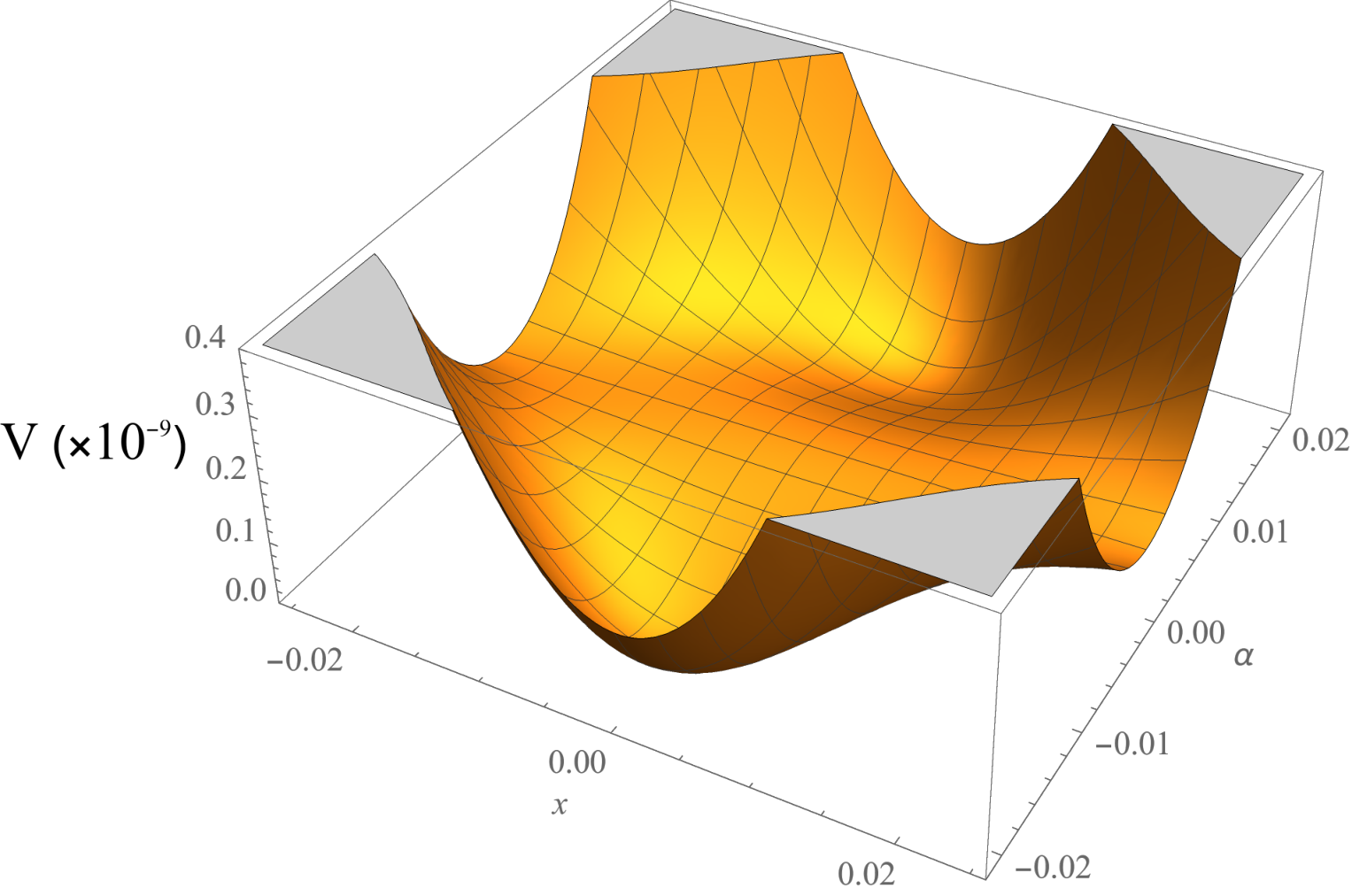
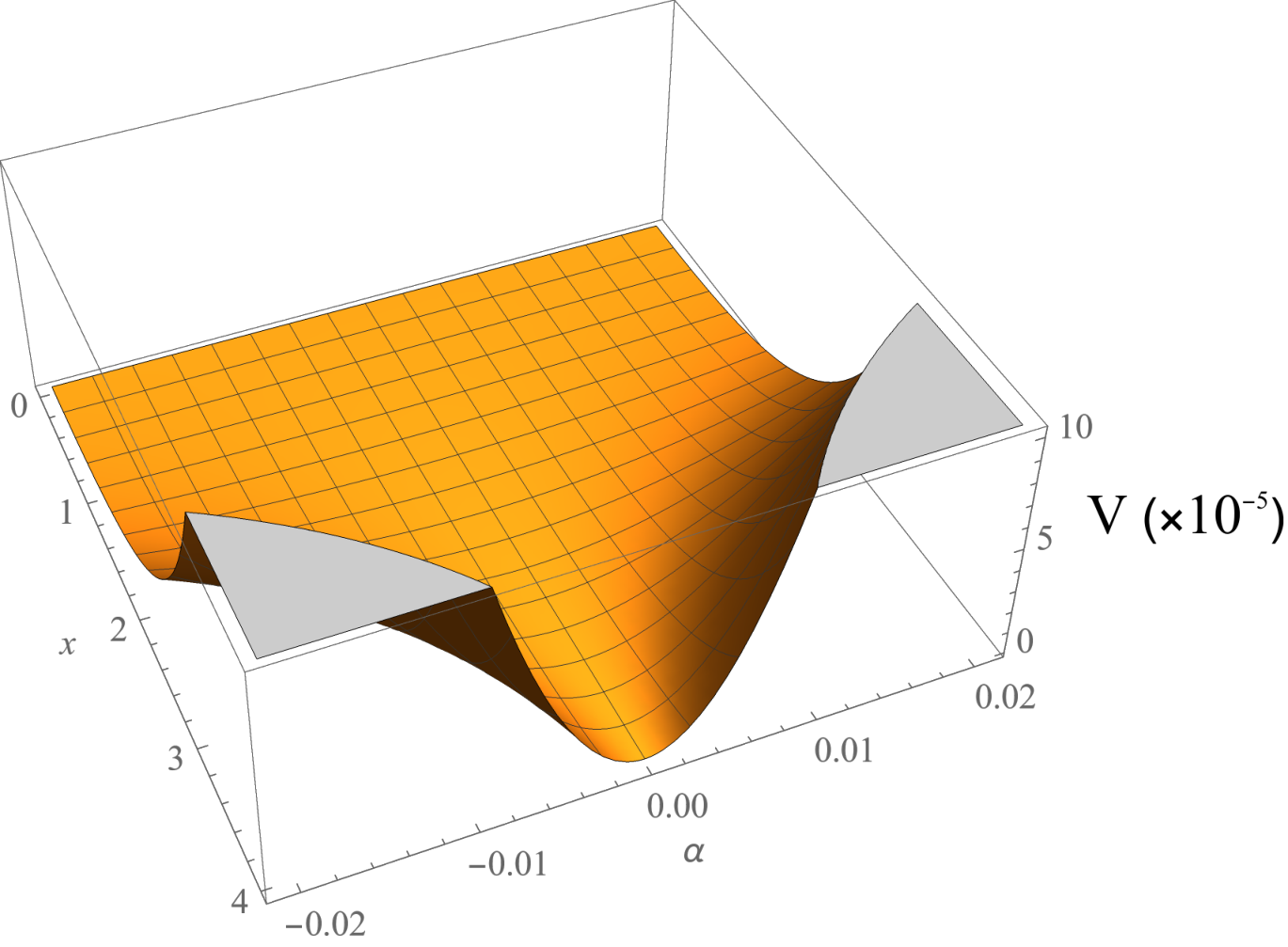
In Fig. 2, we show the potential of . For large values of the potential is minimum direction at and the direction is flat, whereas for small inflation ends and waterfall happens.
We will simulate the time evolution of the scalar fields by solving the supergravity equations of motion:
| (20) | |||
| (21) |
where are the connection coefficients of the Kähler manifold.
Fig. 3 depicts the the simulation of the inflaton which slowly rolls and finally reaches the SUSY minimum at , while the higgs is fixed at zero during inflation then acquires a tachyonic mass hence goes to the SUSY minimum at . On the other hand, are fixed at zero during and after inflation. The time has been rescaled by the Hubble constant .
2.2 Inflaton effective potential
The potential (14) is positive semi-definite and its global minimum is when
| (22) |
Here, it is clear that for , we return to the original ENO model of Ellis:2013xoa. Using the field redefinition (15), the resulting potential will have the form
| (23) |
where
| (24) |
where , are dimensionless quantities. Apparently the simple Starobinsky case (ENO) Ellis:2013xoa, is recovered for . Expanding the hyperbolic functions, considering that is frozen at the origin, the effective inflationary potential will be given by
| (25) |
Clearly, the location of the minimum of the potential at is shifted from the origin once : . The lower sign is chosen such that the minimum is shifted to the left and hence is guaranteed. In that respect, we have the important constrain is satisfied also. The latter allows for the waterfall and hence the fields stabilize to their true minima at , respectively. We study two regimes in the parameter space:
- •
Case I
An interesting case for the inflation potential is the limit when , the potential becomes flat for large values of with constant hight .33 3 In Romao:2017uwa, they considered only the case where and is being a perturbation for ENO model. They infer a restriction from inflation on which gives rise to TeV SUSY breaking scale. It will turn out that is not restricted by inflation to such tiny values, since the potential in the regime has a plateau for large and the former constraint is relaxed to be . In this limit the potential will have the following form
(26) Fig. 4 illustrates the Starobinsky-like potential (25) for the case when the parameters are related as . For the case when (), we restore the Starobinsky inflation case. The minimum will be located at .
- •
Case II:
If , the effective potential (25) can be written as
(27)
Now we turn to discuss the contributions from radiative corrections to the tree-level scalar potential via one-loop Coleman-Weinberg corrections Coleman:1973jx
| (28) |
where the supertrace is taken over all superfields with inflaton dependent masses . As advocated above (2.1), the stabilized fields during the inflation have . Since , the 1-loop correction which is negligible compared to the tree level potential.
2.3 Inflation Observables
Here we will investigate the inflation observables and see the constraints on the different scales and . We investigate the inflation observables such as the tensor-to-scalar ratio , scalar tilt and the scalar amplitude (sensitive to the scale of the inflation), and they can be expressed in terms of the slow-roll parameters and as follows
where the above observables are computed at the crossing horizon value of the inflaton field . The number of efolding is given by
| (29) |
where is the value of the inflaton at the end of inflation. The value of is fixed by observed value of the scalar amplitude at 68% CL Akrami:2018odb. Now we analyze different regimes in the parameter space that leads to successful inflation.
In the limit , we analyze the inflation described by effective potential (26). It is clear that the slow roll parameters depend only on . In that case is given by
| (30) |
This imposes the constrain , such that is positive. The observables and are independent of , and depend only on (see Appendix A). They have the following form
| (31) |
In that case has only upper bound is not fixed by and . If the flat regime is perturbed as , then corresponding potential (27) is not asymptotically flat. Hence, the inflation may not succeed.
In Fig. 6 we show a logarithmic plot for and prediction of the inflationary potential Eq. 25, for both the cases I and II. Changing doesn’t affect the values of and . In particular, the case of , represented by the black dashed segment, and depends only on as demonstrated in Appendix A. We have changed by changing for values of .
Figure 7 depicts the allowed region by the observed value of scalar amplitude , in the plane with fixing . The range of values of . The energy scale of inflation (in the flat potential case I) can be estimated in Planck units as
| (32) |
Therefore the inflation scale is of order GUT scale. For and , the Grand Unification scale is in Planck units. This provides us with a connection between inflation scale, R-symmetry breaking scale that is encoded in the parameters and , and the GUT scale.
3 No scale Hybrid Infation with constant Fayet-Iliopoulos D-terms (FDHI)
In this section we add Fayet-Iliopoulos D-term and study the hybrid inflation by considering the same Kähler potential (6) and the following renormalizable superpotential that breaks R-symmetry
| (33) |
Again is the singlet inflaton superfield while have opposite charges under gauge group which is anomalous or non-anomalous Binetruy:1996xj. The total scalar potential is the sum of the F-term and D-term potentials. Here the D-term is given by
| (34) |
with are Fayet-Iliopoulos D-terms exist for the gauge groups. We consider gauge group and the gauge kinetic function as the Kronecker delta, hence the total potential will be given by
| (35) |
Again the scalar potential is positive semidefinite. The global minimum is supersymmetric and Minkowskian and is corresponding to . It is located at
| (36) |
We will parametrize the complex scalar fields in terms of their real components as follows
| (37) |
One can write in polar representation as with being the vev, hence will correspond to the massless goldstone boson and the dynamics will depend on five real degrees of freedom Heurtier:2015ima. However will work on the basis and is mainly the goldstone boson, hence the minimum of the potential is located at
| (38) |
3.1 Inflation trajectory and effective potential
The scalar potential is minimized in the direction and the effective inflation potential is given by
| (39) |
Clearly, the above potential is the same as the ENO model Ellis:2013xoa but shifted by the energy density . We use the same field redefinition (15), then the target space metric during inflation is found to be diagonal in the basis and is given by
Similarly the fields are fixed at the origin during the inflation, since the scalar potential is minimized for . As a matter of fact, minimizing the potential in the direction of gives two solutions, namely and the other solution for is given by . The latter gives complex value for and the only allowed minimum during inflation is . The field dependent masses are larger than the Hubble scale during inflation as follows
| (40) |
The above equations have been extracted for large values of the inflaton field . In fact the field dependent squared mass matrices of and have mixing terms which are very small in the large limit of the inflaton field. The fields will be fixed at zero during and after inflation. On the other hand will be fixed at during inflation with positive field dependent mass squared. As the inflaton rolling down, its value decreases to smaller values until it reaches a critical value at which the field dependent mass changes to negative and becomes a local maximum. This triggers the waterfall phase and goes to its true minimum. In particular, for small , to leading order . To find the critical value of the inflaton which triggers the waterfall, we expand the masses for small , hence
| (41) |
Accordingly, the critical value at which the sign of flips to negative sign, is given to leading order in by
| (42) |
The effective inflationary potential has a plateau for and is given by
| (43) |
which is the Starobinsky potential shifted by . On the other hand, perturbing the plateau with , the potential is given by
| . | (44) |
Therefore the plateau is spoiled by the last two terms which are very steep. Here we stress that the infation potentials (43,3.1) are only valid for , otherwise the potentials are minimized at with cosmological constant of order which is inconsistent with the observation of infinitesimally small cosmological constant.
Now we turn to discuss the observables. The value of at the end of inflation is
In order to have , the constraint should be satisfied. The shift by doesn’t alter the predictions of the ENO model Ellis:2013xoa, whenever . The scale of inflation is determined by observed value of the scalar amplitude Akrami:2018odb, and is given by
| (45) |
Since the predicted , is of order GUT scale. Figure 8 displays the allowed region by the observed value of scalar amplitude, in the plane with fixing . The range of values of .
4 Moduli backreaction and SUSY breaking
An essential component of the no-scale inflationary models is the modulus field . It turns out that the stabilization mechanism of the modulus field can affect the inflation trajectory Brax:2006ay; Brax:2006yq; Davis:2008fv; Linde:2011ja; Buchmuller:2013uta; Buchmuller:2014vda; Buchmuller:2014pla; Davis:2008fv; Buchmuller:2015oma; Wieck:2014xxa; Dudas:2015lga. In this section we study the effect of the modulus stabilization and the expected backreaction on the inflationary trajectory. We will focus on the mechanism proposed in Ellis:2013nxa; Ellis:1984bs which provides a strong stabilizing terms in the Kähler potential as follows
| (46) |
where the scale such that the modulus acquires large mass and stabilizes during the inflation. The above Kähler potential preserves the no-scale structure with stabilizing the modulus at , where represents the minimum of the modulus in absence of inflation sector. Including the inflation sector, the large positive energy density during inflation shifts the modulus minimum of by . The effective scalar potential is then given, to leading order in , , in terms of the total supergravity scalar potential by
| (47) |
The displacement is obtained by imposing the minimization condition: or equivalently .
It turns out that the exact no-scale symmetry will preserve the inflation potential from dangerous terms such as the soft mass term and the term proportional to Buchmuller:2015oma; Dudas:2015lga. However, the stabilizing term in the Kähler (46) doesn’t have an origin from UV theory such as string theory. If instead we used mechanisms of moduli stabilization in string theory such as KKLT or LVS models, the no-scale structure is broken by the non-perturbative terms in the moduli superpotential and the backreaction of the moduli results in dangerous terms arising from in the scalar potential, which spoils the plateau Dudas:2015lga.
4.1 Backreaction on no-scale FHI
We add a constant to the superpotential (5) and use the Kähler potential (46). At the global minimum, SUSY is broken via the F-term only in the directions of and with zero cosmological constant. The gravitino mass and the modulus mass are given by
| (48) |
On the other hand during the inflation SUSY is broken via D-term and via F-term in the direction of and . The waterfall fields and are still fixed at the origin during the inflation. Hence, the effective potential is given by
| (49) |
As expected, the modulus backreaction on the inflation potential results in corrections suppressed by powers of the large modulus mass which doesn’t affect the plateau.
4.2 Backreaction on no-scale FDHI
Similarly we add a constant to the superpotential (33) and use the Kähler potential (46). At the global minimum, SUSY is broken via the F-term only in the direction of and with zero cosmological constant. The gravitino mass and the modulus mass are given by
| (50) |
On the other hand during the inflation SUSY is broken via D-term and via F-term in the direction of . The effective inflation potential is given by
| (51) |
where the waterfall fields and are still fixed at the origin during the inflation. Again, the modulus backreaction on the inflaton potential is negligible and the plateau is not affected.
5 Reheating
In this section we study the reheating after inflation which is one of the interesting consequences of the FHI model. The mass matrix of the inflaton and the higgs (B) is not diagonal. The mixing between the inflaton and the higgs fields is proportional to . The later is stemming from R-symmetry breaking term in the superpotential (5). This will have important impacts on the reheating scenario. Indeed that provides additional motivation for the inflation scenario 2 where a natural coupling of the inflaton (via the mixing with the GUT higgs) to the the MSSM sector can arise and may contribute to the reheating stage. The mixing angle is given, in terms of the mass matrix (B) entries, by
| (52) |
The physical states (we use the canonical inflaton ) and the physical masses are given as follows
The reheating is dependent on the choice of the gauge symmetry group. We will consider the flipped GUT (FGUT) gauge group (or flipped ) which has many appealing features as well as the advantage of being free from the monopoles tHooft:1974kcl. Inflation and reheating in the context of FGUT scenarios was considered in Gonzalo:2016gey; Kyae:2005nv; Ellis:2017jcp; Ellis:2018moe; Ellis:2019opr. In Gonzalo:2016gey the inflaton was right-handed sneutrino that is charged under FGUT gauge group which allows for natural decay channels to the MSSM particles, while in Ellis:2017jcp; Ellis:2018moe; Ellis:2019opr the inflaton was a singlet. In the latter scenario, it was pointed out a connection between inflation, neutrino masses and reheating via the couplings between the inflaton, the right handed neutrino and the higgs. On the other hand, FGUT hybrid inflation with singlet inflaton was explored in Kyae:2005nv.
The field representations of the flipped group are listed in Table 1 as well as the respective charges. The charges are assigned such that the SM hypercharge is obtained as Gonzalo:2016gey
| (53) |
where is the charge associated with the first abelian factor of the broken , subalgebra of . is the diagonal generator of and .
In this regard the particle content is accommodated in the flipped representations as follows Kyae:2005nv; Ellis:2014xda; Gonzalo:2016gey:
- •
The standard model (SM) matter content is contained in the representations , and as follows
- •
The SM Brout-Englert-Higgs bosons responsible for the electroweak symmetry breaking, are contained in and .
- •
The representations and trigger the breaking of the flipped to the MSSM gauge group by acquiring vevs in the SM neutral direction that are identified with the field :
- •
The inflaton is assigned to a singlet .
| +2 | -2 | -3 | 1 | -1 | 1 | 5 | 0 | 0 | |
| - | + | + | + | + | - | + | + | - |
The complete superpotential which is renormalizable and invariant under and matter parity, is given by
| (54) | |||||
where the indices are the indices. We added matter parity (Table 1), with charge assignments different from those in Kyae:2005nv; Ellis:2014xda; Gonzalo:2016gey, in order to forbid undesirable terms as follows:
- 1.
The bare mass term gives rise to the MSSM mixing term , which is important to trigger the electroweak symmetry breaking in the MSSM and provide the mass for the Higgs superpartners. Indeed a new scale is not protected from being a superheavy scale as the only mass scales in the theory are the GUT and the inflation high scales. Therefore should be put by hand to the SUSY scale to solve the hierarchy problem consistently. This is called the -problem which is a kind of naturalness problem. Hence we forbid this term by symmetry.
- 2.
One may invoke a solution to the MSSM -problem via the gauge invariant term which allows also for decay channels of the inflaton to the higgs. As indicated in Barbieri:1982eh; Dvali:1997uq, the singlet can acquire a non-vanishing vev of order (TeV) if a large expectation value of is triggered, hence SUSY breaking effects shift the vev of to a non-zero value of the same order as the SUSY breaking scale Barbieri:1982eh. However, this solution is a lost cause. In fact the mixing between the inflaton and gives rise to the coupling: which results in a heavy mass term . If the reheating from inflaton decays constrains , then should be which is extremely small and not allowed by the values in the parameter space which are determined by inflation. Nonetheless, the former term is forbidden by symmetry as well.
A natural solution to the MSSM -problem is obtained via Giudice-Masiero (GM) mechanism Giudice:1988yz, or alternatively by putting at tree level and then generating it radiatively Hall:1983iz.
- 3.
The proposed symmetry will forbid higher-dimensional baryon number violating operators such as and , where are flavor indices. Therefore, proton decay will occur via dimension six operators mediated by the supermassive GUT gauge bosons. Accordingly The proton life time predictions are consistent with the observation limits Ellis:2002vk; Dorsner:2004xx; Kyae:2005nv; Ellis:2017jcp.
Moreover, terms such as and are also forbidden by symmetry. These terms may provide heavy masses to and via the terms and .44 4 Here we list some advantages of symmetry which is proposed to allow decay channels for the inflaton to reheat the universe, generate Dirac mass terms for the fermions and neutrinos and prohibit mixing terms of that results in heavy masses for the Higgs. A complete phenomenology of flipped model is beyond the scope of this paper and one can find more details regarding the phenomenology in the literature.
Flipped provides a nice solution to the doublet-triplet splitting problem via the missing partner mechanism Antoniadis:1987dx; Kyae:2005nv. As a matter of fact the the MSSM Higgs pair doesn’t acquire masses throught the vev since the coupling term provides the components of , and the corresponding components of with a superheavy mass scale proportional to the vev . On the other hand, the coupling term is forbidden by symmetry at tree level. However it can be generated at the non-renormalizable level, hence providing the components of , and the corresponding components of with large masses. The components and of and will be absorbed by the gauge bosons to render them massive.
Now we discuss the terms which are relevant to the reheating. The breaking of R-symmetry allows the non-renormalizable term which is invariant under FGUT gauge group. This term gives rise to right-handed neutrino masses and allows for decay channels for the inflaton to right-handed neutrinos and sneutrinos , via the mixing with the FGUT higgs. Hence for GeV and , the right-handed neutrino mass is GeV which is suitable for generating the tiny neutrino masses via type I seesaw mechanism. In that respect, the interaction Lagrangian responsible for the inflaton decay is given by
| (55) |
After diagonalizing the mass matrix (B), we rewrite the Lagrangian (55) in terms of the physical states
| (56) | |||||
The reheating temperature is given by Lazarides:1996dv; Lazarides:2001zd
| (57) |
where is the total decay width of the inflaton field which is given by
| (58) |
An upper bound on the reheating temperature arises from cosmological constraints such as the gravitino overproduction problem Ellis:1984eq; Ellis:1984er; Moroi:1993mb; Kawasaki:2004yh; Antusch:2010mv, and it is given by Antusch:2010mv
| (59) |
Fig. 9 depicts the relation between the reheating temperature and the coupling according to Eq. (57). The GUT scale is fixed with three different values GeV. We have fixed the other parameters with values consistent with the inflation observables: , . The black dotted line gives the cosmological constrain on the reheating temperature. The figure shows that a reheating temperature consistent with the observation bound prefers the GUT scale GeV and . This produces right-handed neutrino masses GeV and inflaton mass GeV, hence the decay is kinematically allowed. The tiny neutrino masses are generated via the seesaw mechanism: , where and is the mixing angle in the MSSM neutral Higgs sector. As hinted by global fit scans deVries:2015hva, , and hence . Therefore, in order to have neutrino masses of the order of eV, , which is typically the same order as the first and second generations. In deed, we may consider the different flavors interactions , hence for up sector Yukawa couplings , . Therefore the inflaton should decay only to the first or second generations in the neutrino sector, as contributions from the the third generation would drive the reheating temperature to values exceeding the the above constrain. We may assume the existence of a flavour violating sector at high energies, without specific details, that prevents the decay to the third generation.
6 Conclusions
In this paper, we have proposed a scenario for hybrid inflation with a maximal breaking of R-symmetry, in no-scale supergravity context. In that respect, we have studied the FHI model and found a region in the parameter space in which the effective potential is asymptotically flat, which is not studied in Romao:2017uwa. We have treated the dynamics of all fields in full detail and realized the waterfall phase. Moreover, we have discussed the case of adding FI D-term which results in an effective potential similar to the ENO model but shifted.
The question of moduli stabilization and their backreaction as well as SUSY breaking has been discussed. It has been emphasised that inflation trajectory will not be affected in specific type of strong moduli stabilization proposed by Ellis et al.
Finally, the reheating phase has been studied in the context of flipped GUT scenario. We have stressed on the role of the associated symmetry in low energy phenomenology and in allowing for decay channels for the inflaton in connection to the neutrino masses. We emphasised that the calculated reheating temperature prefers GUT symmetry breaking scale GeV, in order to be consistent with the cosmological constraints. Moreover the latter constrain implies that the inflaton should decay only to the first or second generations in the neutrino sector, while the third generation should decouple.
Acknowledgments
The work of A. M. is partially supported by the Science, Technology and Innovation Funding Authority (STDF) under grant No. (33495) YRG.
Appendix A No-scale FHI observables
The crossing horizon value of the inflaton as a function in is given by
| (60) |
One can find relations between and as follows
| (61) |
Appendix B Mass matrices
For FHI and in the basis , the target space metric is diagonal at the minimum, and is given by
| (62) |
Therefore the mass squared matrix in the basis , (), is given by
For FDHI, in the basis , the target space metric is diagonal at the minimum, and is given by
Hence the masses are given by
| (68) |
and the mass squared matrix of the other fields is given by
References
- (1) Y. Akrami et al. [Planck], “Planck 2018 results. X. Constraints on inflation,” [arXiv:1807.06211 [astro-ph.CO]].
- (2) M. Kawasaki, M. Yamaguchi and T. Yanagida, “Natural chaotic inflation in supergravity,” Phys. Rev. Lett. 85 (2000), 3572-3575 doi:10.1103/PhysRevLett.85.3572 [arXiv:hep-ph/0004243 [hep-ph]].
- (3) M. Yamaguchi and J. Yokoyama, “New inflation in supergravity with a chaotic initial condition,” Phys. Rev. D 63 (2001), 043506 doi:10.1103/PhysRevD.63.043506 [arXiv:hep-ph/0007021 [hep-ph]].
- (4) P. Brax and J. Martin, “Shift symmetry and inflation in supergravity,” Phys. Rev. D 72 (2005), 023518 doi:10.1103/PhysRevD.72.023518 [arXiv:hep-th/0504168 [hep-th]].
- (5) R. Kallosh and A. Linde, “New models of chaotic inflation in supergravity,” JCAP 11, 011 (2010) [arXiv:1008.3375 [hep-th]].
- (6) L. Heurtier, S. Khalil and A. Moursy, JCAP 10 (2015), 045 doi:10.1088/1475-7516/2015/10/045 [arXiv:1505.07366 [hep-ph]].
- (7) T. E. Gonzalo, L. Heurtier and A. Moursy, “Sneutrino driven GUT Inflation in Supergravity,” JHEP 06 (2017), 109 [arXiv:1609.09396 [hep-th]].
- (8) A. A. Starobinsky, “A New Type of Isotropic Cosmological Models Without Singularity,” Phys. Lett. 91B, 99 (1980); V. F. Mukhanov and G. V. Chibisov, “Quantum Fluctuations and a Nonsingular Universe,” JETP Lett. 33, 532 (1981) [Pisma Zh. Eksp. Teor. Fiz. 33, 549 (1981)]; A. A. Starobinsky, “The Perturbation Spectrum Evolving from a Nonsingular Initially De-Sitter Cosmology and the Microwave Background Anisotropy,” Sov. Astron. Lett. 9, 302 (1983).
- (9) A. D. Linde, “Hybrid inflation,” Phys. Rev. D 49 (1994), 748-754 [arXiv:astro-ph/9307002 [astro-ph]].
- (10) G. R. Dvali, Q. Shafi and R. K. Schaefer, “Large scale structure and supersymmetric inflation without fine tuning,” Phys. Rev. Lett. 73, 1886 (1994). [hep-ph/9406319].
- (11) M. Bastero-Gil, S. F. King and Q. Shafi, “Supersymmetric Hybrid Inflation with Non-Minimal Kahler potential,” Phys. Lett. B 651 (2007), 345-351 [arXiv:hep-ph/0604198 [hep-ph]].
- (12) G. R. Dvali, G. Lazarides and Q. Shafi, “Mu problem and hybrid inflation in supersymmetric SU(2)-L x SU(2)-R x U(1)-(B-L),” Phys. Lett. B 424 (1998), 259-264 [arXiv:hep-ph/9710314 [hep-ph]].
- (13) G. Lazarides and Q. Shafi, “R symmetry in minimal supersymmetry standard model and beyond with several consequences,” Phys. Rev. D 58 (1998), 071702 [arXiv:hep-ph/9803397 [hep-ph]].
- (14) L. J. Hall, J. D. Lykken and S. Weinberg, “Supergravity as the Messenger of Supersymmetry Breaking,” Phys. Rev. D 27 (1983), 2359-2378
- (15) G. F. Giudice and A. Masiero, “A Natural Solution to the mu Problem in Supergravity Theories,” Phys. Lett. B 206 (1988), 480-484
- (16) A. E. Nelson and N. Seiberg, “R symmetry breaking versus supersymmetry breaking,” Nucl. Phys. B 416 (1994), 46-62 [arXiv:hep-ph/9309299 [hep-ph]].
- (17) M. Civiletti, M. Ur Rehman, E. Sabo, Q. Shafi and J. Wickman, “R-symmetry breaking in supersymmetric hybrid inflation,” Phys. Rev. D 88 (2013) no.10, 103514 [arXiv:1303.3602 [hep-ph]].
- (18) S. Khalil, A. Moursy, A. K. Saha and A. Sil, “U(1)R inspired inflation model in no-scale supergravity,” Phys. Rev. D 99 (2019) no.9, 095022 [arXiv:1810.06408 [hep-ph]].
- (19) K. Schmitz and T. T. Yanagida, “Dynamical supersymmetry breaking and late-time R symmetry breaking as the origin of cosmic inflation,” Phys. Rev. D 94, no.7, 074021 (2016) [arXiv:1604.04911 [hep-ph]]. V. Domcke and K. Schmitz, “Unified model of D-term inflation,” Phys. Rev. D 95, no.7, 075020 (2017) [arXiv:1702.02173 [hep-ph]]. V. Domcke and K. Schmitz, “Inflation from High-Scale Supersymmetry Breaking,” Phys. Rev. D 97, no.11, 115025 (2018) [arXiv:1712.08121 [hep-ph]].
- (20) S. Kachru, R. Kallosh, A. D. Linde and S. P. Trivedi, “De Sitter vacua in string theory,” Phys. Rev. D 68, 046005 (2003), [hep-th/0301240].
- (21) V. Balasubramanian, P. Berglund, J. P. Conlon and F. Quevedo, “Systematics of moduli stabilisation in Calabi-Yau flux compactifications,” JHEP 0503, 007 (2005) [hep-th/0502058]; V. Balasubramanian, P. Berglund, J. P. Conlon and F. Quevedo, “Systematics of moduli stabilisation in Calabi-Yau flux compactifications,” JHEP 0503, 007 (2005) [hep-th/0502058].
- (22) E. Cremmer, S. Ferrara, C. Kounnas and D. V. Nanopoulos, “Naturally Vanishing Cosmological Constant in N=1 Supergravity,” Phys. Lett. B 133 (1983), 61.
- (23) J. R. Ellis, C. Kounnas and D. V. Nanopoulos, “No Scale Supersymmetric Guts,” Nucl. Phys. B 247 (1984), 373-395.
- (24) S. Cecotti, “HIGHER DERIVATIVE SUPERGRAVITY IS EQUIVALENT TO STANDARD SUPERGRAVITY COUPLED TO MATTER. 1.,” Phys. Lett. B 190 (1987), 86-92
- (25) R. Kallosh and A. Linde, “Superconformal generalizations of the Starobinsky model,” JCAP 06 (2013), 028 [arXiv:1306.3214 [hep-th]].
- (26) J. Ellis, D. V. Nanopoulos and K. A. Olive, “No-Scale Supergravity Realization of the Starobinsky Model of Inflation,” Phys. Rev. Lett. 111, 111301 (2013) Erratum: [Phys. Rev. Lett. 111, no. 12, 129902 (2013)] [arXiv:1305.1247 [hep-th]].
- (27) M. C. Romao and S. F. King, “Starobinsky-like inflation in no-scale supergravity Wess-Zumino model with Polonyi term,” JHEP 1707, 033 (2017) [arXiv:1703.08333 [hep-ph]]; S. F. King and E. Perdomo, “Starobinsky-like inflation and soft-SUSY breaking,” JHEP 05, 211 (2019) [arXiv:1903.08448 [hep-ph]].
- (28) S. R. Coleman and E. J. Weinberg, “Radiative Corrections as the Origin of Spontaneous Symmetry Breaking,” Phys. Rev. D 7 (1973), 1888-1910
- (29) P. Binetruy and G. R. Dvali, “D term inflation,” Phys. Lett. B 388, 241-246 (1996) [arXiv:hep-ph/9606342 [hep-ph]].
- (30) E. Halyo, “Hybrid inflation from supergravity D terms,” Phys. Lett. B 387 (1996), 43-47 [arXiv:hep-ph/9606423 [hep-ph]].
- (31) P. Binetruy, G. Dvali, R. Kallosh and A. Van Proeyen, “Fayet-Iliopoulos terms in supergravity and cosmology,” Class. Quant. Grav. 21 (2004), 3137-3170 [arXiv:hep-th/0402046 [hep-th]].
- (32) J. Ellis, D. V. Nanopoulos and K. A. Olive, “Starobinsky-like Inflationary Models as Avatars of No-Scale Supergravity,” JCAP 10 (2013), 009 [arXiv:1307.3537 [hep-th]].
- (33) J. R. Ellis, C. Kounnas and D. V. Nanopoulos, “No Scale Supergravity Models with a Planck Mass Gravitino,” Phys. Lett. B 143 (1984), 410-414
- (34) J. Ellis, D. V. Nanopoulos, K. A. Olive and S. Verner, “Phenomenology and Cosmology of No-Scale Attractor Models of Inflation,” [arXiv:2004.00643 [hep-ph]].
- (35) P. Brax, C. van de Bruck, A. C. Davis and S. C. Davis, “Coupling hybrid inflation to moduli,” JCAP 09 (2006), 012 [arXiv:hep-th/0606140 [hep-th]];
- (36) P. Brax, C. van de Bruck, A. C. Davis, S. C. Davis, R. Jeannerot and M. Postma, “Moduli corrections to D-term inflation,” JCAP 01 (2007), 026 [arXiv:hep-th/0610195 [hep-th]]. S. C. Davis and M. Postma, “Successfully combining SUGRA hybrid inflation and moduli stabilisation,” JCAP 04 (2008), 022 [arXiv:0801.2116 [hep-th]]; S. Mooij and M. Postma, “Hybrid inflation with moduli stabilization and low scale supersymmetry breaking,” JCAP 06 (2010), 012 [arXiv:1001.0664 [hep-ph]];
- (37) A. Linde, Y. Mambrini and K. A. Olive, “Supersymmetry Breaking due to Moduli Stabilization in String Theory,” Phys. Rev. D 85 (2012), 066005 [arXiv:1111.1465 [hep-th]].
- (38) W. Buchmüller, V. Domcke and C. Wieck, “No-scale D-term inflation with stabilized moduli,” Phys. Lett. B 730 (2014), 155-160 [arXiv:1309.3122 [hep-th]].
- (39) W. Buchmuller, C. Wieck and M. W. Winkler, “Supersymmetric Moduli Stabilization and High-Scale Inflation,” Phys. Lett. B 736 (2014), 237-240 [arXiv:1404.2275 [hep-th]].
- (40) W. Buchmuller, E. Dudas, L. Heurtier and C. Wieck, “Large-Field Inflation and Supersymmetry Breaking,” JHEP 09 (2014), 053 [arXiv:1407.0253 [hep-th]].
- (41) W. Buchmuller, E. Dudas, L. Heurtier, A. Westphal, C. Wieck and M. W. Winkler, “Challenges for Large-Field Inflation and Moduli Stabilization,” JHEP 04 (2015), 058 doi:10.1007/JHEP04(2015)058 [arXiv:1501.05812 [hep-th]].
- (42) S. C. Davis and M. Postma, “SUGRA chaotic inflation and moduli stabilisation,” JCAP 03 (2008), 015 [arXiv:0801.4696 [hep-ph]].
- (43) C. Wieck and M. W. Winkler, “Inflation with Fayet-Iliopoulos Terms,” Phys. Rev. D 90 (2014) no.10, 103507 [arXiv:1408.2826 [hep-th]].
- (44) E. Dudas and C. Wieck, “Moduli backreaction and supersymmetry breaking in string-inspired inflation models,” JHEP 10 (2015), 062 [arXiv:1506.01253 [hep-th]].
- (45) G. ’t Hooft, “Magnetic Monopoles in Unified Gauge Theories,” Nucl. Phys. B 79 (1974), 276-284.
- (46) J. Ellis, T. E. Gonzalo, J. Harz and W. C. Huang, “Flipped GUT Inflation,” JCAP 03 (2015), 039 [arXiv:1412.1460 [hep-ph]].
- (47) I. Antoniadis, J. R. Ellis, J. S. Hagelin and D. V. Nanopoulos, “Supersymmetric Flipped SU(5) Revitalized,” Phys. Lett. B 194 (1987), 231-235; A. Masiero, D. V. Nanopoulos, K. Tamvakis and T. Yanagida, “Naturally Massless Higgs Doublets in Supersymmetric SU(5),” Phys. Lett. B 115 (1982), 380-384; B. Grinstein, “A Supersymmetric SU(5) Gauge Theory with No Gauge Hierarchy Problem,” Nucl. Phys. B 206 (1982), 387.
- (48) J. R. Ellis, D. V. Nanopoulos and J. Walker, “Flipping SU(5) out of trouble,” Phys. Lett. B 550 (2002), 99-107 [arXiv:hep-ph/0205336 [hep-ph]].
- (49) I. Dorsner and P. Fileviez Perez, “Distinguishing between SU(5) and flipped SU(5),” Phys. Lett. B 605 (2005), 391-398 [arXiv:hep-ph/0409095 [hep-ph]].
- (50) B. Kyae and Q. Shafi, “Flipped SU(5) predicts delta T/T,” Phys. Lett. B 635 (2006), 247-252 [arXiv:hep-ph/0510105 [hep-ph]].
- (51) J. Ellis, M. A. G. Garcia, N. Nagata, D. V. Nanopoulos and K. A. Olive, “Starobinsky-like Inflation, Supercosmology and Neutrino Masses in No-Scale Flipped SU(5),” JCAP 07 (2017), 006 [arXiv:1704.07331 [hep-ph]].
- (52) J. Ellis, M. A. G. Garcia, N. Nagata, D. V. Nanopoulos and K. A. Olive, “Symmetry Breaking and Reheating after Inflation in No-Scale Flipped SU(5),” JCAP 04, 009 (2019) [arXiv:1812.08184 [hep-ph]].
- (53) J. Ellis, M. A. G. Garcia, N. Nagata, D. V. Nanopoulos and K. A. Olive, “Superstring-Inspired Particle Cosmology: Inflation, Neutrino Masses, Leptogenesis, Dark Matter \& the SUSY Scale,” JCAP 01, 035 (2020) [arXiv:1910.11755 [hep-ph]].
- (54) R. Barbieri, S. Ferrara and C. A. Savoy, “Gauge Models with Spontaneously Broken Local Supersymmetry,” Phys. Lett. B 119 (1982), 343; A. H. Chamseddine, R. L. Arnowitt and P. Nath, “Locally Supersymmetric Grand Unification,” Phys. Rev. Lett. 49 (1982), 970; H. P. Nilles, M. Srednicki and D. Wyler, “Weak Interaction Breakdown Induced by Supergravity,” Phys. Lett. B 120 (1983), 346 L. J. Hall, J. D. Lykken and S. Weinberg, “Supergravity as the Messenger of Supersymmetry Breaking,” Phys. Rev. D 27 (1983), 2359-2378
- (55) G. Lazarides, R. K. Schaefer and Q. Shafi, “Supersymmetric inflation with constraints on superheavy neutrino masses,” Phys. Rev. D 56 (1997), 1324-1327 [arXiv:hep-ph/9608256 [hep-ph]].
- (56) G. Lazarides, “Inflationary cosmology,” Lect. Notes Phys. 592 (2002), 351-391 [arXiv:hep-ph/0111328 [hep-ph]].
- (57) J. R. Ellis, J. E. Kim and D. V. Nanopoulos, “Cosmological Gravitino Regeneration and Decay,” Phys. Lett. B 145 (1984), 181-186 doi:10.1016/0370-2693(84)90334-4
- (58) J. R. Ellis, D. V. Nanopoulos and S. Sarkar, “The Cosmology of Decaying Gravitinos,” Nucl. Phys. B 259 (1985), 175-188 doi:10.1016/0550-3213(85)90306-2
- (59) T. Moroi, H. Murayama and M. Yamaguchi, “Cosmological constraints on the light stable gravitino,” Phys. Lett. B 303 (1993), 289-294 doi:10.1016/0370-2693(93)91434-O
- (60) M. Kawasaki, K. Kohri and T. Moroi, “Hadronic decay of late - decaying particles and Big-Bang Nucleosynthesis,” Phys. Lett. B 625 (2005), 7-12 doi:10.1016/j.physletb.2005.08.045 [arXiv:astro-ph/0402490 [astro-ph]].
- (61) S. Antusch, J. P. Baumann, V. F. Domcke and P. M. Kostka, “Sneutrino Hybrid Inflation and Nonthermal Leptogenesis,” JCAP 10 (2010), 006 doi:10.1088/1475-7516/2010/10/006 [arXiv:1007.0708 [hep-ph]].
- (62) K. J. de Vries, E. A. Bagnaschi, O. Buchmueller, R. Cavanaugh, M. Citron, A. De Roeck, M. J. Dolan, J. R. Ellis, H. Flächer, S. Heinemeyer, G. Isidori, S. Malik, J. Marrouche, D. Martinez Santos, K. A. Olive, K. Sakurai and G. Weiglein, “The pMSSM10 after LHC Run 1,” Eur. Phys. J. C 75 (2015) no.9, 422 [arXiv:1504.03260 [hep-ph]].