Perturbation Theory of Optical Resonances
of Deformed Dielectric Spheres
Master’s Thesis in Physics
Presented by
Julius Gohsrich
September 1, 2020
Friedrich–Alexander–Universität Erlangen–Nürnberg
![[Uncaptioned image]](2009.14003v1/pics/fau-siegel.jpg)
| Supervisor: | Prof. Dr. Florian Marquardt |
|---|---|
| Co-Supervisor: | Dr. habil. Andrea Aiello |
Abstract
Light injected into a spherical dielectric body may be confined very efficiently via the mechanism of total internal reflection. The frequencies that are most confined are called resonances. If the shape of the body deviates from the perfect spherical form the resonances change accordingly. In this thesis, a perturbation theory for the optical resonances of such a deformed sphere is developed. The optical resonances of such an open system are characterized by complex eigenvalues, where the real part relates to the frequency of the resonant light and the imaginary part to the energy leakage out of the system. As unperturbed and analytically solvable problem serves the homogeneous dielectric sphere, and the corrections to its eigenvalues are determined up to and including second order for any polarization of light. For each order, the corrections of the optical resonances are determined by a finite-dimensional linear eigenvalue equation, similar to degenerate time-independent perturbation theory in quantum mechanics. Furthermore, geometrically intuitive applicability criteria are derived. To check the validity of the presented method, it is applied and compared to an analytically solvable problem.
1 Introduction
The description of light scattering from dielectric bodies like, e.g., raindrops, atmospheric dust, crystals, et cetera, is an active topic for over a century. The first exact mathematical solution was derived by Gustav Mie in his seminal 1908 work [1] concerning dielectric spheres. Until today, Mie theory remains an active topic with applications ranging from microscopic resonators to astrophysics [2].
One of the most remarkable phenomenon described by this theory is the occurrence of optical resonances. A resonance manifests as a sharp peak in the total scattering cross-section of the scatterer and can be explained by resonances of the underlying structure. For a dielectric sphere, such resonant behavior can be explained by whispering gallery modes (WGMs), which propagate close to the inner surface due to near-total internal reflection [3, 4, 5]. As some light leaks out of the dielectric sphere, such a system can be described as an open system, characterized by complex eigenvalues of an associated non-Hermitian operator [6, 7, 8].
The WGMs are used in a plethora of optical and optomechanical applications. Microscopic glass spheres are used to realize biological, chemical and physical sensors [9, 10]. In such systems, the WGMs probe the surface of the dielectric body as well as objects close to the surface, and small deviations from the spherical form drastically change the frequencies and the losses of the WGMs. Such deviations are the result of the manufacturing process as well as due to surface roughness and are in general unwanted. For optomechanical systems using levitated drops of liquids on the other hand, the surface of the droplet acts as mechanical resonator and therefore is needed to change its shape. Furthermore, flattening due to rotation, thermally excited capillary waves and other surface waves deforms the surface of such droplets [11]. Figure 1.1 illustrates an arbitrarily deformed dielectric body.
Due to the increasing interest in such optical and optomechanical systems, a wealth of numerical [12, 13] and perturbative methods have been developed to determine the resonances of such slightly deformed dielectric spheres. The most sophisticated perturbative methods are the resonant state expansion (RSE) [14, 15, 16] and the Kapur-Peierls (KP) formalism [17]. Both of these methods originate in the quantum theory of scattering [18, 19]. The RSE uses an optical analogue of Gamow [20] or Siegert [21] states and employs Brillouin-Wigner perturbation theory. While this approach is well-suited for numerical considerations, an order of perturbation, and thus the notion of error estimation, does not exist. On the other hand, the KP formulation employs Rayleigh-Schrödinger perturbation theory which does not suffer from this weakness, however it makes use of some strong assumptions and is not able to predict corrections of transverse magnetic modes. Furthermore, both approaches do not deliver applicability criteria.

In order to overcome those shortcomings, we want to employ another perturbative method called Boundary Condition Perturbation Theory (BCPT), the progenitor of the popular Rayleigh-Schrödinger perturbation theory. It was originally developed by Lord Rayleigh in his book The Theory of Sound [22], where he investigated how the mechanical resonances of a circular membrane change if it gets slightly deformed. Recently, this method has successfully been applied to effective two-dimensional cavities, which slightly deviate from a circular form [23, 24, 25].
The general idea of BCPT is quickly outlined: First one needs to find the general solution of the electromagnetic fields, solely depending on a set of field coefficients and an eigenvalue. The boundary condition encodes the geometry and thus some small parameter. By inserting the general solution into the boundary condition and expanding the boundary condition around the small parameter, one finds a chain of equations relating the field coefficients, the resonances, and their respective corrections. Solving this chain of equations order by order determines the optical resonances. This approach differs significantly from the ones in the current literature, where the boundary condition is brought into a particular simple form allowing to shift the problem to an expansion of the electromagnetic fields.
Employing BCPT we are able to determine the optical resonances up to and including second-order corrections for any polarization of light including geometrically intuitive applicability criteria. We remark that, at the best of our knowledge, the second-order perturbative solutions for both TE- and TM-polarizations of the electromagnetic fields, were never derived, in a correct form, before. Thus, the results presented in this thesis are perfectly original and solve a long-standing open problem.
This thesis is structured as follows. In Section 2 we determine the electromagnetic fields solving Maxwell’s equations for a dielectric body embedded in another dielectric material. Considering the boundary condition appropriate for the dielectric sphere we determine its optical resonances. Having solved the unperturbed problem, we generalize our approach in Section 3 by considering a more general boundary condition, encoding the geometry of a more general dielectric body, and bring it to a form suitable to apply BCPT. In Sections 4 and 5 we finally apply BCPT and determine the optical resonances of such a dielectric body up to and including second-order corrections for both polarizations of light. In Section 6 we rewrite the first-order equations in a more explicit way and reason the validity of our method by applying and compare it to an analytically solvable problem in Section 7. We conclude our work in Section 8.
2 Resonances of a Dielectric Sphere
Before we tackle the hard problem of finding the optical resonances of a deformed dielectric sphere, we need to understand the general physical framework and the unpertubed problem, the dielectric sphere.
We start by adapting Maxwell’s equations to our problem in Section 2.1. Following that, we introduce the Debye potentials to derive a general solution for Maxwell’s equations in Section 2.2. Afterwards we refine the Debye potentials so that they describe physical fields in Section 2.3 and finally find the optical resonances for a perfectly spherical body in Section 2.4.
2.1 Maxwell’s Equations for a Dielectric Body
In classical electrodynamics, Maxwell’s equations describe the evolution of electromagnetic fields. Considering the fields inside a dielectric medium, Maxwell’s equations read
| (2.1) | ||||
where the dot denotes the time derivative and all vector fields depend on . Let us consider a dielectric body, the interior of which defines a region , made of a homogeneous isotropic dielectric material (medium ) surrounded by another one (medium ). Both media are separated by the interface denoted . As we have two regions, we label them by , so corresponds to medium inside , and corresponds to medium outside .
Maxwell’s equations in this form are incomplete and need to be completed by the constitutive equations, which relate the electromagnetic fields and with and . In this work we assume a linear response described by
| and | (2.2) |
Here, is the vacuum permittivity, the relative permittivity, the vacuum permeability and the relative permeability. As the speed of light in vacuum is and the speed of light in matter is , we introduce the refractive index
| (2.3) |
Throughout this work, we will assume that . Collecting the previous statements and assuming time-harmonic fields, i.e., all fields vary as , we can rewrite Maxwell’s equations as
| (2.4a) | ||||
| (2.4b) | ||||
| (2.4c) | ||||
| (2.4d) | ||||
where the fields lost their time dependence and only depend on . In this form it is apparent that Maxwell’s equations are invariant under the discrete transformation
| and | (2.5) |
which is called dual symmetry and will help us finding new results out of old ones.
Sometimes it is useful to decouple Maxwell’s equations. By taking the curl of (2.4c), using the vector identity on the left hand side of the equation and inserting (2.4d) on the right side of the equation, one finds the vector Helmholtz equation
| (2.6) |
which can be physically interpreted as time-independent wave equation for the electric field. Employing the dual symmetry (2.5), one finds that the magnetic field also satisfies the Helmholtz equation.
If one assumes plane wave solutions of (2.6), i.e., the fields are proportional to , Helmholtz’s equation gives us the well-known dispersion relation
| (2.7) |
where the wave number in matter is given by and denotes the vacuum wave number.
As partial differential equations, Maxwell’s equations need to be accompanied by boundary conditions. In the context of electromagnetic interfaces, these are also called matching conditions and can be determined to be
| and | (2.8) |
where is the normal of .
2.2 Debye Potentials
Now we want to find a general solution for Maxwell’s equations (2.4). Every divergenceless electromagnetic field can be split into [26]
| (2.9a) | |||
| (2.9b) | |||
where is the orbital angular momentum operator11 1 A list of all properties of the angular momentum operator used in the work can be found in Appendix B of [26].
| (2.10) |
The scalar fields and are the so-called (scalar) Debye potentials [27] and respectively encode two different polarized fields, namely the transverse electric (TE)
| (2.11) |
and transverse magnetic (TM) ones
| (2.12) |
The names come from the fact that the TE polarized part of the electric as well as the TM polarized part of the magnetic field are transverse to the radial direction , i.e.
| (2.13) |
This is also called a toroidal field. In addition to that, the respective remaining part of the electromagnetic field are poloidal fields satisfying
| (2.14) |
Furthermore, the fields of the same polarization are orthogonal to each other
| (2.15) |
The fields described by (2.9) satisfy the first two Maxwell equations (2.4a-2.4b) by definition, as
| (2.16) |
The remaining equations (2.4c-2.4d) are fulfilled if the Debye potentials satisfy the scalar Helmholtz equation
| (2.17) |
where denotes the polarization. Thus we found that by introducing the Debye potentials, we reduced the two vector Helmholtz equations (2.6) for the electromagnetic fields to two scalar Helmholtz equations for the Debye potentials.
Before we actually solve this equation, let us write the electromagnetic fields in terms of the Debye potentials in a more suitable way. First we notice from the form of (2.9) that the dual symmetry of Maxwell’s equations (2.5) can be expressed using the Debye potentials as
| (2.18) |
where the square brackets denote functional dependence. With this property we can restrict our discussions to one of the two fields. As the next step, we expand the Debye potentials in their Laplace series (B.5) as
| (2.19) |
where are the scalar spherical harmonics and we denote with the reduced Debye potentials. Inserting Laplace’s series into from (2.11) we find
| (2.20) |
where in the second line we used the fact that commutes with any functions solely depending on and in the third line we introduced the vector quantity , which will be defined soon. Using
| (2.21) |
where , we can rewrite the transverse magnetic part of the electric field in (2.12) as
| (2.22) |
where in the second line, we used from (B.1). In the last line and in (2.20) we introduced the three vector quantities
| and | (2.23) |
called vector spherical harmonics. It can be shown that the vector spherical harmonics are orthogonal [28] and complete [29] and therefore permit a multipole expansion of the electromagnetic fields as
| (2.24a) | ||||
| (2.24b) | ||||
where we reintroduced the label and used (2.18) to get the magnetic field. Furthermore we want to draw attention to the fact that the sum over actually starts at , since , as well as the prefactor of vanish. Up to this point, the reduced Debye potentials are not yet specified.
2.3 Physical Fields
In the previous section, we brought the electromagnetic fields in the form (2.24) and showed that they satisfy Maxwell’s equations if the Debye potentials satisfy the scalar Helmholtz equation (2.17). Multiplying (2.17) by and rewriting the Laplacian in terms of the angular momentum operator using (A.9), we find
| (2.25) |
Inserting Laplace’s series for from (2.19) and using the product rule results in
| (2.26) |
and finally substituting one finds
| (2.27) |
which is the spherical Bessel (differential) equation (cf. App. D). Its fundamental solutions are the spherical Bessel functions and and the general solution is the superposition of both
| (2.28) |
Another way to express this solution is by employing the spherical Hankel functions and from (D.3) to write
| (2.29) |
The physical solutions however are more restrictive. Let us first consider the reduced Debye potentials inside the dielectric body (). Here we have to require that the Debye potentials are everywhere regular. As the spherical Bessel function of second kind diverges at the origin ( for ), the everywhere regular solution is given by (2.28) with .
For the Debye potential outside (), the linear combination of the spherical Hankel functions (2.29) is suited best, as in the far field, they describe outgoing spherical waves ( for ) and incoming spherical waves ( for ). Thus, the physical solutions need to be of the form
| (2.30a) | ||||||
| (2.30b) | ||||||
These reduced Debye potentials, and therefore the corresponding electromagnetic fields, describe a scattering process: The incident field is encoded in , the scattered field in and the internal field in . Such a scattering problem can be symbolically solved by introducing the transition matrix connecting the incident field coefficients with the scattered field coefficients via
| (2.31) |
and the boundary condition (2.8) encoding the geometry of the problem fully determines the transition matrix [29]. This -matrix encodes all physical relevant information, however, only the -matrix of the dielectric sphere is analytically known in our setup.
The resonances, characterized by sharp peaks in the total scattering cross-section, are associated to the analytic continuation of the -matrix [30, 29]. As the -matrix, and therefore its poles, is in general not analytically known, one has to find a different approach to determine the resonances.
One possibility to determine the resonances was introduced by Gamow in the context of quantum mechanical scattering theory [20]. By imposing outgoing waves only, in our case setting in (2.30) to zero, one can determine the resonances without determining the -matrix. For electromagnetic scattering, this idea was already used in [15, 16] to construct the resonant-state expansion. Using Gamow’s approach has two important implications for us. The first one is that the resonances are characterized by complex eigenvalues, where the imaginary part relates to the energy leakage out of the dielectric body . This is in contrast to the scattering solutions described in the previous paragraphs, where the wave numbers are real. The second implication is that the associated electromagnetic fields are not physical as they are not normalizable in the standard sense[31, 32]. Usually, this problem needs to be addressed by constructing some non-standard normalization in order to determine the resonances. In this work however, we find the resonances without introducing such a normalization. We demonstrate this fact for the dielectric sphere in the next section.
Before we do so, let us write down the electromagnetic fields for explicitly. Therefore we insert (2.30) into (2.24). To distinguish the Gamow approach from the scattering approach, we rename and and find for the fields inside the dielectric body
| (2.32) |
and
| (2.33) |
where we rewrote the -component using
| (2.34) |
It can be shown that the vector quantities in the square brackets in (2.3) and (2.3) are part of a complete set called regular spherical vector waves [29].
Similarly one has for the electromagnetic fields outside the dielectric body
| (2.35) |
and
| (2.36) |
where we dropped the superscript in as the spherical Hankel function of second kind does not occur anymore. Likewise to the regular spherical vector waves, the quantities in square bracket are denoted out-going or radiating spherical vector waves.
To conclude this section let us remark that at no point in the derivation of the electromagnetic fields we made any assumption on the form of the dielectric body. Thus, all information needs to be encoded in the field coefficients and , which will be determined by imposing the electromagnetic boundary conditions (2.8) at the interface between the two dielectric media.
2.4 Resonances of the Dielectric Sphere
Let us start to develop our perturbative approach by finding the resonances of the dielectric sphere with radius . To do so we need to rewrite the general boundary conditions (2.8). Using the fact that the normal is given by , the boundary conditions can evidently be rewritten as
| and | (2.37) |
Inserting the multipole expansions (2.3,2.3,2.3,2.3) into these boundary conditions, we find
| (2.38) |
and
| (2.39) |
where we used the cross products of with the vector spherical harmonics given by (C.6)
| and | (2.40) |
From the orthogonality of the vector spherical harmonics (C.3) it follows that each square bracket in (2.4) and (2.4) that multiplies a vector spherical harmonics must vanish. Due to the linear independence of and , the first line of (2.4) results in
| and | (2.41) |
and the first line of (2.4) gives
| and | (2.42) |
where and are arbitrary complex constants depending on and . Substituting (2.42) into the second line of (2.4) we obtain the condition for the TE modes
| (2.43) |
and by inserting (2.41) into the second line of (2.4), we likewise find the condition for the TM modes
| (2.44) |
These equations precisely describe the values for , for which the -matrix introduced in the previous section becomes singular [29]. Thus by assuming outgoing waves only, we found the resonances of the dielectric sphere without the need to determine the -matrix first. Furthermore, an overall normalization of the electromagnetic field is not needed.
To proceed further, let us introduce the dimensionless wave number
| (2.45) |
which we denote in anticipation of further calculations as eigenvalue of the system. With this, we have and we furthermore introduce the functions
| (2.46a) | ||||
| (2.46b) | ||||
so that we can compactly rewrite (2.43) and (2.44) as
| and | (2.47) |
respectively. These transcendental equations can be solved numerically and a detailed discussion is presented in [17], Appendix B. We briefly discuss the approach in Figure 2.1. The most important properties of the resonances are that they are complex numbers with negative imaginary part, and we express this fact writing , where . Furthermore, one finds for each and a countably infinite set of resonances labeled by as . From the analytic continuation of and in (D.6) it follows that , and thus the resonances are symmetrically distributed around the imaginary axis. Therefore, one can label the resonances with positive real part with positive as
| (2.48) |
and the resonances with negative real part satisfying where . The spectrum for TE-modes is shown in Figure 2.2. All the resonances are intrinsically non-degenerate with respect to , and , but quasi-degeneracies occur [23]. In the context of quantum mechanical scattering theory, the resonances with negative real part are denoted as anti-resonances [33].

Finally, let us discuss the modes associated to the resonances. The Debye potentials associated with the resonances are given by
| (2.49a) | ||||
| (2.49b) | ||||
and
| (2.50a) | ||||
| (2.50b) | ||||
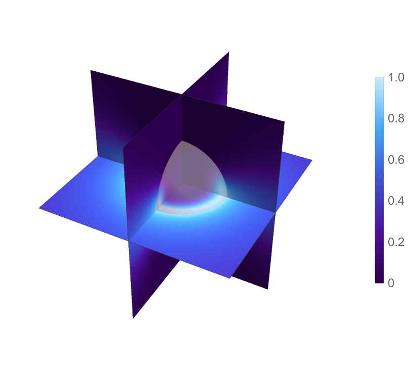
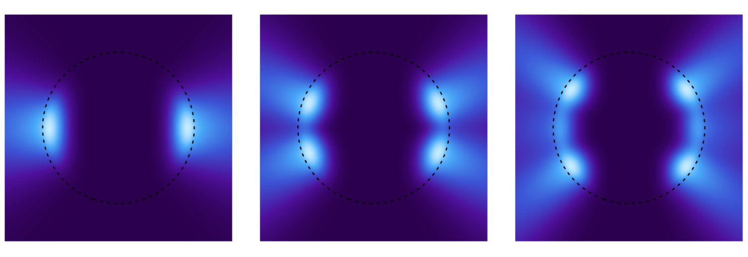
and the associated electromagnetic modes can be obtained by inserting them into (2.24). The TE-modes are visualized in Figures 2.3, 2.4 and 2.5. These Debye potentials show the general complication of assuming outgoing waves only. If one considers the far field and again splitting with results in
| (2.51) | ||||||
As the second factor tends to infinity, the Debye potentials as well as the associated electromagnetic modes are not normalizable in a standard sense and the coefficients stay undetermined. However, when deriving the formula for the resonances, there was no need for any normalization or any restriction on the coefficients. We will exploit this fact in further considerations.
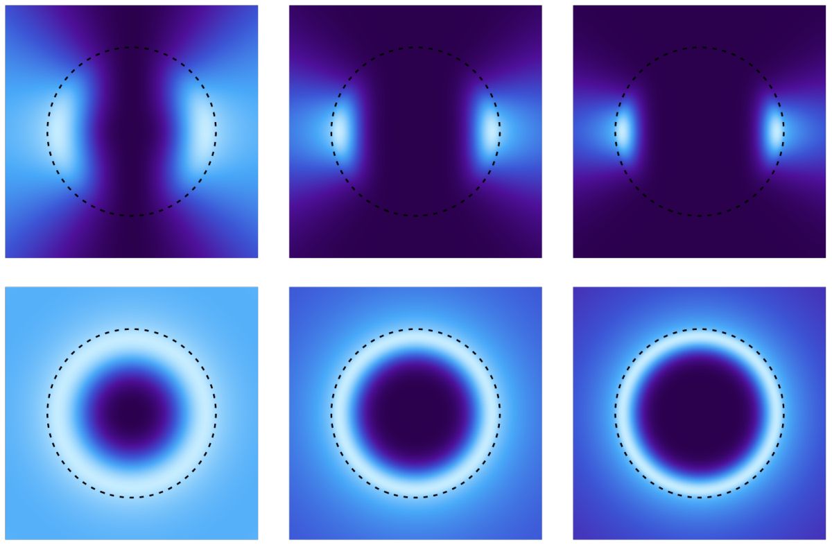
Top row: Side view of the WGMs. For increasing , the WGMs are more localized at the equator. Furthermore the losses occur more and more only in the plane of the equator. Bottom row: Corresponding top views at the equator. This again visualizes the increasing localization at the equator.
3 Generalization of the Problem
In the previous section we introduced the general physical fields which solve Maxwell’s equations for an arbitrarily shaped dielectric body within another dielectric medium. By imposing outgoing waves only, we found the resonances of a perfectly spherical body. This work is dedicated to apply this approach to dielectric bodies the form of which deviate from a perfect spherical one.
In order to find the resonances of such non-spherical bodies, we analyze the geometry of this generalized problem in Section 3.1. With that, we can discuss in Section 3.2 the perturbative approach we choose to find the resonances of our problem: The Boundary Condition Perturbation Theory (BCPT). To be able to employ the BCPT later on, we rewrite the boundary condition in Section 3.3. As the perfectly spherical body serves as unperturbed problem, it will be the starting point for our perturbative treatment and thus we solve this problem again in Section 3.4 using the newly derived boundary conditions.
3.1 The Geometry
As the main aim of this section is to derive suitable boundary conditions, let us recall the appropriate boundary conditions (2.8) for this problem
| and |
From the boundary conditions it is apparent that they depend on the geometry of the dielectric body , which is encoded in the form of the dielectric interface and its normal .
To be able to do calculations, we have to choose a suitable parametrization for the dielectric interface . One possibility is to introduce the surface profile function
| (3.1) |
where is a constant and the deformation function is a smooth, single-valued function of and defined on the unit sphere . Figure 3.1 illustrates the surface profile function. The form of this parametrization seems suitable for a perturbative approach, because one can interpret as the radius of a sphere and creates a supposedly small deviation from the perfect sphere. Using this parametrization it makes sense to denote the body as a deformed sphere.
Before we continue, let us state that the form of (3.1) is not the most general parametrization, as we assume a smooth, single-valued . However, for the physical applications we have in mind, both requirements are met if one sets the center of the deformed sphere to the origin. In Section 3.2.1 we reason that if we drop one or both of these requirements, the perturbation theory we employ will most likely fail.

In view of a perturbation theory, it is useful to introduce a supposedly small expansion parameter. In this setup, we define the deformation strength as
| (3.2) |
and if we require to be small, this translates to
| (3.3) |
Using the deformation strength, (3.1) can be rewritten as
| (3.4) |
where . We will show in Section 3.2.1 that (3.3) is not sufficient to apply the perturbation theory.
Using the surface profile function, we can rewrite the boundary conditions as
| and | (3.5) |
To progress further, we want to determine the normal of the deformed sphere . Let us write down the interface implicitly as
| (3.6) |
where
| (3.7) |
Here we again see that for , we have the implicit definition of a sphere with radius . By acting with the nabla operator (A.7) on (3.7) [34], we find the normal
| (3.8) |
where we introduced
| (3.9) |
It needs to be understood that the subscript denotes quantities that are parallel to the surface of undeformed sphere and are therefore orthogonal to . Let us finally introduce an -independent vector , defined as
| (3.10) |
so (3.9) can be rewritten as
| (3.11) |
3.2 Boundary Condition Perturbation Theory
To motivate our further steps, let us discuss how we want to solve our problem. In the previous section we chose a parametrization for a deformed dielectric sphere in dependence of a supposedly small parameter .
The method to solve our problem is BCPT, originally developed by Lord Rayleigh in his book The Theory of Sound [22], where he investigated how the modes of a circular membrane, and therefore the pitch of the emitted sound, changes if one slightly deforms the membrane22 2 When considering the deformed circular membrane, one has to solve Helmholtz’s equation in polar coordinates for a fixed boundary in order to determine the (scalar) sound waves as well as the (real) eigenvalue of the system. In our case, we have to consider two three-dimensional vector fields, which we can reduce to the Debye potentials satisfying Helmholtz’s equation. However, the three-dimensional character as well as the boundary condition introduces lots of complications. For simpler boundary conditions, cf. [35]..
The idea behind BCPT is pretty clear. By expanding the boundary condition around the supposedly small parameter , one gets a chain of equations for all orders in . Here, the zeroth order equation corresponds to the boundary condition of the unperturbed problem, which solution is analytically known. By successively solving the chain of equations, one finds a perturbative solution of the problem.
Let us motivate BCPT by applying it to the current form of our boundary conditions (3.5). By expanding the normal from (3.8) as
and using
for the field evaluated at the boundary, we can rewrite the boundary condition for the electric field as
Here we immediately see that the zeroth order boundary condition corresponds, as expected, to the boundary condition of the undeformed sphere discussed in Section 2.4. Now one might be able to use the general zeroth-order result and insert it in the first-order equation,
| (3.12) |
to refine the result. It turns out that solving the problem in this form, if it is even possible, is inconvenient, and we need to adapt the boundary condition to fit our needs in Section 3.3.
3.2.1 Applicability of BCPT
However, this outline reveals a problem. Recalling the definition of ,
from (3.10), we see that the derivatives of with respect to and might be huge, a situation that is denoted as a strongly winding boundary condition [25]. This has the effect that the first term in (3.12) might be of the same order of magnitude as the zeroth order, and the perturbative approach breaks down.
This rises the question, when BCPT is applicable and when it is not. Let us derive a criterion, for which the perturbative expansion is valid. We define
| (3.13) | ||||
where denotes the norm of a vector and the maximum over the sphere . This parameter encodes both troublesome derivatives. As we want the first term in (3.12) to be of order unity, we have to require
| (3.14) |
in order for the BCPT to hold. We can also give this criterion a geometrical meaning by considering the angle between the normal vector of the undeformed sphere and the normal vector of the deformed sphere. We compute
where we used properties of the normal from Section 3.1 and neglected terms of higher orders in in the third line. Therefore, encodes the lower bound of . By imposing (3.14) we finally get
| (3.15) |
or in other words, is almost parallel to . Therefore, our criterion is equivalent to the requirement of local paraxiality.
This also brings us back to the choice of our parametrization of the boundary of Section 3.1. There we choose the deformation function to be smooth and single-valued due to our physical intuition of the problem. Now we can further reason, why we chose these requirements. If we do not require smoothness of , is ill-defined. Likewise to this, a multi-valued will violate the local paraxiality. This does not exclude the possibility to get the BCPT working when dropping one or both of the requirements, but strongly suggests that this needs further considerations.
For the remainder of this work, we will assume that (3.14) holds and thus consider as bona fide expansion parameter.
3.3 Reformulation of the Boundary Conditions
We now want to rewrite the boundary conditions in a way which will be suitable to employ the BCPT. We will do this in two steps. The first one is to remove a redundancy in the boundary conditions. The second step is to use the explicit form of the electromagnetic fields from Section 2.3 to express the boundary condition in terms of the field coefficients.
3.3.1 Removing Redundancy
For the perfect spherical boundary condition in Section 2.4, we expressed the electric and magnetic field in terms of the vector spherical harmonics and also had . This enabled us to use
| and |
from (C.6) to simplify the boundary condition. This had the effect that the -components of the fields do not contribute to the actual boundary condition. This gives us the hint that there might be some redundancy in the boundary condition.
Going to the perturbed problem, the normal in the boundary condition of the deformed sphere additionally contains and . Thus, one also has to determine the cross products of those basis vectors with the vector spherical harmonics, which cannot be expressed as simple as in (C.6).
To resolve both of these points, one can write the electromagnetic fields in spherical coordinates (A.3). Let us choose the electric field as example, i.e.
| (3.16) |
and also rewrite the normal vector (3.8) as
| (3.17) |
Using this, one can immediately rewrite the boundary condition (3.5) for the three components as
| (3.18a) | ||||
| (3.18b) | ||||
| (3.18c) | ||||
where we used (A.6), and all coefficients need to be evaluated at . Now it is not hard to show that only two of these three equations are independent. For example
| (3.19) |
Let us choose (3.18b) and (3.18c) as independent equations. Following [36], we multiply (3.18b) by , (3.18c) by and summing these two equations, we obtain a single vector equation,
| (3.20) |
which needs to be evaluated at the boundary. Here, corresponds to the definition in (3.9), and we introduced
| (3.21) |
similar to , parallel to the surface of the undeformed sphere. With these calculations we on the one hand removed redundancy from the boundary conditions33 3 So this was no special feature of the boundary conditions of the undeformed sphere. In general, the electromagnetic boundary conditions are redundant [37]., on the other hand, avoided evaluating the cross products.
Now we want to build the bridge back to the multipole expansion. As and as well as are orthogonal to it (C.7), encodes the radial part of the field and together with encode the parallel part .
As these considerations similarly hold for the magnetic field, we summarize both boundary conditions for later reference as
| (3.22a) | ||||
| (3.22b) | ||||
3.3.2 Derivation of a Matrix Equation
Now that we removed redundancy from the boundary condition and found (3.22), we can insert the general form of the electromagnetic fields into it and therefore find a boundary condition connecting the field coefficients.
Let us recall the multipole expansions of the fields inside (2.3,2.3)
| (3.23) | ||||
| (3.24) |
| (3.25) | ||||
| (3.26) |
of the dielectric sphere. Here we introduced the radial functions , with and , defined as
| (3.27) | ||||
Recalling the boundary conditions (3.22) from Section 3.3.1, we need to know the parallel part of the fields and the radial part . Following the argument of the previous section, we exemplary find the electric field inside the deformed sphere
Hence, collecting all terms, the boundary condition for the electric field (3.22a) reads
| (3.28) |
which needs to be evaluated at , and here and hereafter,
| stands for | (3.29) |
Likewise, the boundary condition for the magnetic field (3.22b) reads
| (3.30) |
Let us define vector quantities, suggested by the round brackets of both previous boundary conditions, as
| (3.31a) | ||||
| (3.31b) | ||||
where . Again we employ a multipole expansion to move the entire angular dependence to the vector spherical harmonics at the cost of an infinite sum. As we have no radial component in this equation anymore, the vector spherical harmonic does not occur and we find
| (3.32a) | ||||
| (3.32b) | ||||
where the coefficients can be determined using (C.5) via
| (3.33a) | ||||
| (3.33b) | ||||
with being either or . Again, as and vanish, the term does not contribute to (3.32) and thus does not need to be determined by (3.33). Substituting (3.32) into the boundary conditions (3.3.2) and (3.3.2), we find
| (3.34) |
and
| (3.35) |
From the orthogonality of the vector spherical harmonics (C.3) it follows that we need to satisfy for each and the following four homogeneous equations:
| (3.36a) | ||||
| (3.36b) | ||||
| (3.36c) | ||||
| (3.36d) | ||||
We can now rewrite these equations in the suggestive matrix form
| (3.37) |
where we introduced the perturbation matrix
| (3.38) |
as well as the (field-) coefficients vector
| (3.39) |
We want to emphasize that the matrix formulation of the boundary condition in (3.37) is exact. Admittedly, it contains infinite sums and, as we have to consider all and , infinitely many equations. However, this boundary condition is favorable compared to previous formulations, as it does not include any radial or angular dependence and is a single, non-redundant equation. Additionally, it is a set of linear equations and we have a wealth of mathematical tools to solve problems of this kind.
3.4 The Unperturbed Problem
To get further convinced of the usefulness of our new boundary condition, let us consider the unperturbed problem. As the spherical boundary is described by and therefore , we can substitute this into (3.31) to find
| and | (3.40) |
where we added the superscript to distinguish quantities of the unperturbed problem from the general ones. As the entire angular dependence is encoded in the vector spherical harmonics, we can employ their orthogonality (C.3) to determine the perturbation matrix elements using (3.33). A straight-forward calculation gives
| (3.41a) | ||||
| (3.41b) | ||||
| (3.41c) | ||||
| (3.41d) | ||||
By going back to the definition of the radial functions (3.27) we find and recalling that the radial functions actually depend on , we again introduce the dimensionless wave number . For later convenience, let us define to rewrite the matrix equation (3.37) in the case of an undeformed sphere as
| (3.42) |
where we performed the infinite sum over and using the Kronecker deltas in (3.41) and renamed the indices and . We again write it compactly as
| (3.43) |
This linear equation allows two types of solutions, the trivial one, characterized by a non-vanishing determinant of the system, and the non-trivial solutions, characterized by a vanishing determinant. To calculate the determinant, we notice that the perturbation matrix is block-diagonal, i.e.,
| (3.44) |
With this property, it is clear that the boundary condition does not mix and with and , i.e., the boundary condition does not mix TE- and TM- modes. This property also allows the factorization of the determinant via
| (3.45) |
To calculate the determinant of both matrices, we recall the definitions of and the equations (2.46) to find
| and | (3.46) |
Hence the determinant of the joint system reads
| (3.47) |
This sets us in the same situation as in Section 2.4: On the one hand, we get the trivial solution of (3.43) if is no eigenvalue of the perfectly spherical body. On the other hand, the non-trivial solutions are the TE- or TM-resonances characterized by . Thus, we find full agreement of both approaches.
4 Resonances of a Deformed Dielectric Sphere:
TE-Case
Equipped with the boundary condition encoded in the matrix equation (3.37), we can conveniently employ BCPT and determine the resonances of slightly deformed dielectric spheres. Since the treatment of TE-resonances allow simplifications compared to the TM-resonances, we determine the corrections of TE-resonances in this section, and the correction of the TM-resonances in Section 5.
To determine the corrections to the TE-resonances, we first introduce a quantum-like notation and do some initial discussions in Section 4.1. With this, we are able to solve the first-order equations conveniently in Section 4.3. As the result of the first-order equations allow two distinct higher-order approaches, we study them separately in in Sections 4.4 and 4.5 and find the resonances of the perturbed system up to and including second-order terms.
4.1 Introduction of a Quantum-like Notation
To solve the full boundary condition (3.37) in an efficient and clear manner, it is convenient to adopt a quantum-like notation to represent the coefficients and the variables of this equation. The use of such a notation is possible because one can always associate a linear operator to a matrix and vice versa. However, we should always keep in mind that we are dealing with a purely classical physics problem, even though we are using quantum-like notation.
4.1.1 Construction of the Hilbert Space
To begin with, let us introduce the states with and . By hypothesis, they are orthonormal
| (4.1) |
and form an orthonormal basis of the infinite-dimensional Hilbert space that we denote as . The resolution of identity for this space reads
| (4.2) |
and expresses its completeness. Here and hereafter, the subscript denotes operators in and the caret symbol will mark operators in any infinite-dimensional Hilbert space.
Next we define the four vectors with . We also impose that they are orthonormal,
| (4.3) |
and span a four-dimensional Hilbert space denoted as . The completeness of this basis is again granted by the resolution of identity
| (4.4) |
where the identity operator can be represented by the identity matrix.
Finally we define the tensor product Hilbert space
| (4.5) |
which is by definition spanned by the vectors
| (4.6) |
The completeness relation for then reads:
| (4.7) |
where here and hereafter operators in will be denoted by calligraphic letters and the caret again indicates the infiniteness of the associated Hilbert space. From now on we will write the triple sums in a more compact way as in (3.29), so
| stands for | (4.8) |
4.1.2 Derivation of an Operator Equation
Equipped with this paraphernalia, we can rewrite our full boundary condition (3.37) in terms of states and operators in .
To do so, we first introduce the vector state to be represented by the coefficients vector defined in (3.39), i.e.,
| (4.9) |
where we use the symbol to denote a vector or matrix representation. As usual, we can go from the abstract state to the vector representation by multiplying a basis state from the left, and we define
| (4.10) |
Here, denotes the component of the vector , as
| (4.11) |
Secondly, we want to define the perturbation operator so that by acting with it on we reproduce (3.37). Therefore, we define the matrix elements of the perturbation operator in terms of the matrix elements of the perturbation matrix as
| (4.12) |
where, in comparison with (3.38), we have for example
| and |
Using this notation, we can equivalently rewrite (3.37) as
| (4.13) |
We can show this by inserting an identity (4.7) left and right of and find
4.1.3 Application of BCPT
Now we want to apply BCPT using this quantum-like notation. In Section 3.2 we discussed that the idea is to expand the boundary condition, and therefore all quantities in (4.13), in powers of a supposedly small parameter . To this end, we start by doing some purely formal manipulations, without worrying about the convergence of the power series.
Let us start by expanding the state as
| (4.14) |
Similarly we want to expand the perturbation operator , where the eigenvalue encodes the optical resonance of the perturbed system. In the light of customary perturbation theories we first expand in powers of as
| (4.15) |
and introduce the expansion of the perturbation operator
| (4.16) |
Since from (4.15), we notice that the zeroth-order perturbation operator can be rewritten as
| (4.17) |
Now that we expanded the state in (4.14) as well as the perturbation operator in (4.16), we can insert them into the boundary condition (4.13). We find
We can solve this equation perturbatively by requiring that each term in this equation needs to vanish separately. Thus we find the chain of equations
| (4.18a) | ||||||
| (4.18b) | ||||||
| (4.18c) | ||||||
which we need to solve successively to determine the resonance as well as the field coefficients encoded by up to the desired order.
This sets in a similar situation as in quantum mechanics, where the analogous perturbative approach is called Rayleigh-Schrödinger perturbation theory, also known as time-independent perturbation theory or stationary state perturbation theory (cf., e.g., [38]). This is due to the fact that the underlying Hilbert space structure is compatible. However, besides this mathematical similarity, the underlying physics encoded in the operators and states is completely different.
4.1.4 Properties of the Perturbation Operator
Let us remark up to now this is only a formal expansion and we did not use any properties of the perturbation operator. However, as we defined it in terms of the matrix elements of the perturbation matrix in (4.12), and the matrix elements are given by (3.38), one can explicitly calculate them. As these computations are rather lengthy and not very insightful, they are presented with full details in Appendix E. To progress, we want to summarize the most important results of these computations. The first noticeable one is that we actually find an expansion as depicted in (4.16). The second result is that we can rewrite the zeroth-, first- and second-order perturbation operators as
| (4.19a) | ||||
| (4.19b) | ||||
where denotes first- and second-order operators. These newly introduced operators have further properties. The first one addresses the operators , where denotes all orders considered in this work. They are diagonal with respect to the basis vectors , that is,
| (4.20) |
and the operator can be represented by a matrix. By multiplying with from the left, one finds its matrix elements
| (4.21) |
where especially is represented by defined in (3.43).
The second property of the operators and is that they are independent of , which we write as
| and | (4.22) |
Simply speaking, this property states that the entire -dependence of in (4.19b) is explicitly written down.
4.2 Zeroth-Order Perturbation Theory
Let us now use our quantum-like notation by solving the zeroth order equation (4.18a). We can rewrite this equation using (4.19a) as
| (4.23) |
By inserting two resolutions of identity (4.7) left and right of we find
| (4.24) |
where we used (4.20), defined in the second line and carried out the summation over and in the last one. Since the form a complete basis of , all the coefficients in the square bracket need to be identically zero. That is
| (4.25) |
Of cause, this is the same result that we would had obtained if we just multiplied (4.23) from the left by and we will use this property heavily later on. As previously stated, in basis has the matrix representation defined by (3.43) and is represented by the vector . Hence the previous equation is equivalent to
| (4.26) |
But this sets us exactly in the same situation as for the unperturbed problem, discussed in Section 3.4, if we require , i.e., the zeroth-order eigenvalue has to be a valid eigenvalue of the unperturbed problem. This confirms our physical expectation that the zeroth-order perturbation theory reproduces the unperturbed problem. Thus, we can now interpret as an unperturbed eigenvalue and the quantities and as its first- and second-order corrections respectively.
To continue, let us write (4.26) in its full form as
| (4.27) |
We recall from Section 2.4 that the solutions of this equation are characterized by the resonances , where , and . Let us now choose the specific TE-mode .
From the aforementioned section we know that (4.27) is trivially solvable if . Together with the fact that the resonances are non-degenerate with respect to , we find for . Thus, the last step is to solve (4.27) for . To do so, we first find that the TE-modes are characterized by
where we recalled (2.47) and the definition of from Section 3.4. Now it is useful to introduce
| (4.28) |
to rewrite (4.27) for compactly as
| (4.29) |
From the first line we find that and then the second line gives a trivial identity. The remaining two lines give , as the determinant of the magnetic block is non-zero due to the fact that the resonances are non-degenerate with respect to the polarization as discussed in Section 2.4.
Now that we fully solved the zeroth order, let us summarize the results. By choosing an unperturbed eigenvalue , we found the field coefficients
| and | (4.30) |
Up to now, the coefficients are completely arbitrary real or complex numbers.
4.2.1 Change of Basis
The four-dimensional basis defined by (4.3), although natural, is not the most suitable basis for further considerations. In the previous paragraphs we noticed that we have a vanishing determinant in the electric block which results in the trivial identity in the second line of (4.29). To exploit this property we diagonalize the electric block. Let us consider the operator in , which encodes the electric block. In basis , , it is given by
| (4.31) |
where was defined in (3.44). First of all we notice that this matrix, and therefore also the operators and , is non-Hermitian. To handle this in a convenient way, we employ bi-orthogonal states, which is a method heavily used in quantum mechanics when considering open systems, characterized by non-Hermitian Hamiltonians [6, 7, 8].
The idea of this method is to introduce two sets of eigenvectors of , the right-eigenvectors and the left-eigenvectors , so that
| (4.32a) | ||||
| (4.32b) | ||||
In the case of non-Hermitian operators, one has in general . It is not hard to show that these eigenvalue equations are satisfied by
| (4.33a) | ||||||
| (4.33b) | ||||||
with and . By writing these vectors we have chosen the standard normalization for bi-orthogonal vectors, that is
| (4.34) |
and by inspection we also find
| (4.35) |
where the identity operator is represented by the identity matrix. Thus we found that our bi-orthogonal states form a complete basis of .
We now want to promote this new basis to a complete basis of . Therefore we simply extend the vector representation of our state by padding it with two zeros, e.g.,
| (4.36) |
They get completed by defining44 4 An alternative possibility would be to fully diagonalize defined by (4.29), but this is not necessary and not practically convenient.
| and | (4.37) |
It is an elementary algebra exercise to verify that these basis vectors also satisfy the standard normalization condition for bi-orthogonal vectors,
| (4.38) |
and form a complete basis of , i.e.,
| (4.39) |
By construction, we diagonalized the electric block of (4.29) and kept the magnetic block, so in the new basis we have
| (4.40) |
where the determinant of the lower matrix is non-vanishing.
With our new basis we can also rewrite our zeroth-order result. To do so, we rewrite our zeroth-order state as
| (4.41) | ||||
| (4.42) |
where we used (4.30) in the second line and (4.6) in the last one. However, we notice that
| (4.43) |
and we can conveniently write (4.41) as
| (4.44) |
where we introduced
| (4.45) |
It needs to be understood that the states are the fundamental solutions of our unperturbed problem, that is,
| (4.46) |
and likewise, the bi-orthogonal conjugate expression satisfies the conjugate zeroth-order equation
| (4.47) |
4.2.2 Some Preparatory Remarks
In the previous section we found that all are solutions of the zeroth-order equation (4.46), and the zeroth-order result is an undetermined linear combination of those states. The reason for this is that the unperturbed resonance is -fold degenerate with respect to . We need to take this fact into consideration when solving the higher-order equations.
To treat the degeneracy55 5 There is no non-degenerate case as . in a convenient and clear manner, let us consider the states
| (4.48) |
in associated to . These states span a -dimensional subspace of which we denote as degenerate subspace . With this, we can split into a part contained in and a part contained in its complementary subspace via
| (4.49) |
where here and hereafter
| stands for | (4.50) |
Mathematically speaking, in (4.49) we split into a projection on the degenerate subspace and a projection on the complementary subspace.
From our zeroth-order considerations we found it convenient to use the basis in , so we rewrite (4.49) as
| (4.51) |
To get a series expansion of as in (4.14), we introduce a shorthand notation for the scalar products and expand them. In the degenerate subspace, we have
| (4.52) |
and in the non-degenerate subspace we have
| (4.53) |
with . With this definitions, we immediately find the zeroth-order results
| and | (4.54) |
In order to solve the higher-order equations, we collect our previous results and find
| (4.55) |
With this, we are fully equipped to solve the first-order equation.
4.3 First-Order Perturbation Theory
Let us start by recalling the equation under consideration (4.18b). Together with (4.19), it reads
| (4.56) |
In order to solve this equation, we project onto the degenerate and non-degenerate subspace as discussed in the previous section.
4.3.1 First-Order Eigenvalue Corrections
Let us start by considering this problem in the degenerate subspace. Therefore we multiply (4.56) from the left with to find
| (4.57) |
which needs to hold for all and . Recalling the zeroth-order result (4.46), we find that the first term vanishes for . Let us consider this specific case first. Inserting our zeroth-order state from (4.44) yields
| (4.58) |
Now we can use (4.21) to exploit the diagonal form of and do some straight forward manipulations to get66 6 The division by is always possible as .
| (4.59) |
This is nothing but an eigenvalue equation, which we rewrite as
| (4.60) |
Here we introduced the matrix with elements
| (4.61) |
and going through the explicit calculations in Section 6.1, it turns out that is a Hermitian matrix. Furthermore, we defined the -component vector with components
| (4.62) |
and the, due to the Hermicity of , real eigenvalues as
| (4.63) |
In this formulation it is clear that we find eigenpairs solving (4.60), and we label them with as
| (4.64) |
Thus we finally write (4.60) as
| (4.65) |
With this, we found the first-order eigenvalue corrections.
To proceed, we notice that the deformation is encoded in and that we can consider two cases separately. The first one is the non-degenerate case, where for all , i.e., all first-order eigenvalue corrections are different. The second case is the degenerate case, where we have for some . Until Section 4.5, let us assume that the perturbation fully removed the degeneracy, i.e., we consider the non-degenerate case.
4.3.2 Normalization and another Basis Change
The next step is to discuss the eigenvectors of the Hermitian matrix . First we recall that from (4.62), which means that the first-order eigenvalue equation (4.65) determines the zeroth-order coefficients .
Furthermore we did not rely on any normalization of the electromagnetic fields, and thus on any constraint on the , to determine the unperturbed eigenvalues as well as the corresponding first-order eigenvalue corrections. Due to the Hermicity of , the are orthogonal and it will be advantageous to choose them orthonormal as
| (4.66) |
and we will see soon, why this helps us to keep the calculations close to the quantum-mechanical Rayleigh-Schrödinger perturbation theory.
To proceed, we notice that the dictate a new basis of . Let us consider the states
| (4.67) |
in the degenerate subspace . Using the orthogonality of the states from (4.1) as well as the orthogonality of the from (4.66), it immediately follows that these states are orthonormal
| (4.68) |
and due to the completeness of the in , we also find that these states are complete
| (4.69) |
where denotes the identity operator in . Thus, the states form a complete and orthonormal basis of .
As always, we can use this basis to build a basis for via
| (4.70) | ||||
| (4.71) |
and we also define its conjugate . With these definitions it is easy to show that the form a complete and orthonormal basis of .
This new basis is natural in the sense that it has useful properties to conveniently treat the problem. First of all, the states are solutions of the zeroth-order equation (4.23), i.e.,
| and | (4.72) |
This just clearly expresses the fact that we do not know ab initio which is the correct linear combination of to consider to find the desired eigenvalue. After we solved the first-order equation however, we know that
| (4.73) |
depending on which eigenvalue correction we consider77 7 We could also introduce an index to and to label this this dependence, however, we choose not to do so in order to keep a more compact notation..
Furthermore, the are not only the correct zeroth-order states to begin with, but they also diagonalize via
| (4.74) |
Now let us consider a specific eigenvalue correction . Thus, the corresponding zeroth-order state is
| (4.75) |
and its bi-orthogonal conjugate zeroth-order state is
| (4.76) |
This unperturbed state is normalized according to
| (4.77) | ||||
| (4.78) |
This is the result of our choice, that the are orthonormal, but has no straightforward physical meaning. This is different from quantum mechanical perturbation theories, where the wavefunction needs to be properly normalized to have its well-known probabilistic interpretation.
Before we continue, let us use our new basis for by rewriting (4.55) as
| (4.79) |
and we likewise introduce the expansion coefficients
| (4.80) |
Using this change of basis, the zeroth-order result reads
| and | (4.81) |
4.3.3 First-Order State Corrections
In order to solve the second-order equation in the next section, we also need to determine the first-order state corrections encoded in . Therefore we need to fully solve the first-order equation (4.56).
Let us start to solve the first-order equation in the degenerate subspace first. Therefore we multiply it with from the left and recall that we consider the eigenvalue correction setting the zeroth-order state as in (4.75). We find
| (4.82) |
Before we can solve this equation, we need to notice that the matrix elements of in the new basis are given by
| (4.83) |
which directly follow from the diagonality of in (4.20) as well as the orthonormality of the in (4.68). With this, we can now determine all terms in (4.82) separately.
Starting with the first term using (4.79), we find
| (4.84) |
where in the second line, we dropped the term due to (4.40). The second term of (4.82) equals
| (4.85) | ||||
where we simplified the term using (4.74) and get no simplifications for . The third and last term is proportional to
| (4.86) |
Now that we determined all three terms separately, we can collect them and find after some elementary manipulations
First of all we notice that we get a trivial identity for the case using (4.40) for the left hand side. This just confirms that we are doing things consistently, as we already used this case to construct the basis . Additionally we notice that the coefficients are left undetermined in the first-order perturbation theory.
To find the remaining coefficients in the degenerate subspace, let us write down the case separately as
| (4.87) |
By noticing that can be represented by the invertible matrix depicted in (4.40), we can solve for the with by inversion.
In contrast to these calculations, the determination of the coefficients in the non-degenerate subspace seems trivial. First of all, we project (4.56) on the non-degenerate subspace and find for all , and
| (4.88) |
Again we consider all terms separately. Using (4.79), the first term is given by
| (4.89) |
For the second term, no simplification can be made and the last term vanishes due to the diagonality of . Therefore we find
| (4.90) |
Similar to the previous case, we can represent as invertible, this time , matrix defined in (4.26) and again solve for the by inversion.
4.4 Second-Order Perturbation Theory
Now we want to determine the second-order correction to the eigenvalue , still only for TE-resonances under the assumption that the deformation removed the degeneracy at first order discussed in Section 4.3.1.
First of all, let us bring the second-order equation (4.18c) using (4.19) into our familiar form
| (4.91) |
4.4.1 Second-Order Eigenvalue Corrections
Likewise to our first-order calculations, we multiply (4.91) with from the left and find
| (4.92) |
Again we factor out this equation and determine all five contributions separately.
To determine the first term, we notice that the are solutions of the conjugate zeroth-order equation depicted in (4.72) and thus, the first term vanishes. For the second term, we simply decompose the first-order state correction as in (4.79) to write this term as
| (4.93) |
where we separated the sum into its and contribution in the second line and used (4.74). The third term without its prefactor is given by
| (4.94) | ||||
| (4.95) |
where we again split the sum into two contributions and did not carry out the summation over for later convenience. The fourth term allows no simplification and the fifth and final one is proportional to
| (4.96) |
Collecting all pieces together and rearranging the terms we find
| (4.97) |
By choosing , we can solve this equation the second-order eigenvalue correction via
| (4.98) |
As all quantities on the right hand side of this equation are either known first-order coefficients or known matrix elements, this equation actually gives us the second-order eigenvalue correction.
Finally, let us introduce likewise to our first-order considerations
| (4.99) |
in order to rewrite the eigenvalue of the perturbed system (4.15) up to second order as
| (4.100) |
where both and have an implicit dependence on the unperturbed resonance. This concludes our search for the perturbed TE-eigenvalues if the perturbation removes the degeneracy at first order.
4.4.2 Further Remarks
At this point it should be clear how to determine higher-order corrections. However, there is one detail left to discuss.
In order to determine the third-order eigenvalue correction, and similarly for higher orders, one actually has to determine the up to now unknown coefficients . Therefore we recall that we still have to solve (4.97) for the case . In the case that the deformation fully removes the perturbation, the prefactor does not vanish. Therefore we can solve this equation via
| (4.101) |
where again all quantities on the right-hand side are already known. However, there is still the undetermined first-order quantity . To find it, we impose the normalization of the perturbed state as
| (4.102) | ||||
and together with our zeroth-order normalization from (4.77), we therefore need
| (4.103) |
Now we can insert our zeroth-order state as well as our first-order state correction from (4.79) to find
| (4.104) |
where we used the orthogonality of our states. At this point, we determined all first-order quantities.
Let us remark that the normalization (4.103) is in quantum mechanics known as the intermediate normalization and the wavefunction renormalization has to be applied in order to keep the probabilistic interpretation of the wavefunction. However, as discussed in Section 4.3.2, the overall normalization of the state is arbitrary and we can choose it for our convenience.
Now we want to discuss the first-order correction to . First let us recall the rather complicated spectrum of the perturbation operator in . By construction, this Hilbert space is spanned by the vectors . Let us write them down as
We knew from our zeroth-order calculation that our zeroth-order state had to be a linear combination of the basis states colored blue in the equation above. Apart from that, also contains the basis states , , colored black in the equation above. The fact that these states also lie in is a choice, as we denote as the degenerate subspace and not .
When we changed the basis, we were simply rearranging the vectors in without affecting the space , so we have
where we highlighted in blue the zeroth-order state of which we calculate the perturbative corrections. By going to the first order in perturbation theory, we found that our zeroth-order state gets a correction. Especially all states in black in the above equation get multiplied by their corresponding .
Furthermore, gets corrections from the states , , which are in the non-degenerate subspace. As their basis does not get changed, they simply get multiplied by .
To conclude this discussion, we want to write the perturbed state up to first order in its full form as
| (4.105) |
4.5 Degenerate Second-Order Perturbation Theory
Now that we have computed the second-order eigenvalue correction under the assumption that all first-order eigenvalue corrections are all different, we want to drop this assumption and generalize our approach to geometries which do not have this property. For example, an oblate spheroid has rotational symmetry and keeps a two-fold degeneracy at all orders [5].
4.5.1 Modification of the First-Order Eigenvalue Equation
To find this generalization, we first of all need to reconsider the first-order eigenvalue equation (4.65). The standard technique to handle the degenerate eigenvalues is to go from a single label indexation to a two label indexation . This gives us the flexibility to rewrite the first-order eigenvalue equation as
| (4.106) |
where labels the different first-order eigenvalues so that for all , which is equivalent to for all , and labels the corresponding eigenvectors with a -fold multiplicity. These are potentially different for each , but need to satisfy
| (4.107) |
In the present case, the perturbation does not fully remove the degeneracy, but reduces the -fold degeneracy of the zeroth-order eigenvalue to a -fold degeneracy at first order. After noticing this, the next steps are completely analogue to the ones in Section 4.3.1.
First of all, we choose the eigenvectors orthonormal
| (4.108) |
and likewise, they dictate a new orthonormal and complete basis of via
| (4.109) |
similar to the previously. Again, for these states are solutions of the zeroth-order equation
| and | (4.110) |
as well as they diagonalize via
| (4.111) |
Using this new basis, we can decompose our full state similar to (4.79) into its part contained in and its part contained in the complementary subspace via
| (4.112) |
and we introduce the shorthand notations
| and | (4.113) |
Even though we found a basis to handle our problem more conveniently, this time our zeroth-order state is not yet completely determined. By fixing and checking the limit
| (4.114) |
using (4.112) we find the zeroth order-state
| (4.115) |
where the coefficients are still undetermined. In this form it should be clear that the degenerate case we currently consider is a generalization of the non-degenerate case: If we pick an eigenvalue labeled by which is non-degenerate, i.e., , then the sum collapses and we are in the same situation as in the non-degenerate case.
4.5.2 The First-Order State Corrections
In order to determine the second-order eigenvalue corrections, we have to determine the first-order corrections to the perturbed state. The only difference to non-degenerate case is that we need to consider the zeroth-order state given by (4.115) as well as the new basis states in the degenerate subspace.
This time we start with the non-degenerate case. By multiplying our first-order equation (4.56) with , , we find
| (4.116) |
We already understand that we can represent as an invertible matrix. In anticipation of our second-order calculations, we explicitly solve this equation for the . To do so, we multiply the previous equation by and sum with respect to . We find
| (4.117) |
where we relabeled . The most important observation is that the are linear combinations of the, up to now, unknown zeroth-order coefficients .
Secondly we want to solve the first-order equation in the degenerate subspace. Therefore we multiply (4.56) from the left with . Similar to our previous consideration, we find a trivial identity and
| (4.118) |
where , which is the analogue of (4.87). Again, we can solve this equation by inversion for , , and find that they are a linear combination of the .
4.5.3 Second-Order Eigenvalue Corrections
Finally we want to determine the second-order eigenvalue corrections . To find them, we multiply (4.91) from the left with and find the analogue of (4.97) with ,
| (4.119) |
Let us recall from our first order considerations that as well as are just linear combinations of the unknown zeroth-order coefficients. Thus every single term in (4.119) depends on the unknown zeroth-order coefficients, and we can rewrite this equation as an eigenvalue equation
| (4.120) |
where is a -matrix, a -component vector and we similarly to define
| (4.121) |
Similar to our first-order considerations, we introduce the label to denote the eigenvalues and we write
| (4.122) |
With this, we can rewrite the eigenvalue of the perturbed system likewise to (4.100) as
| (4.123) |
In this form it is clear that the zeroth-order eigenvalue is degenerate with respect to and , the first-order correction removes the degeneracy with respect to and the second-order correction removes the degeneracy with respect to . This concludes our search for perturbed eigenvalues up to and including second-order corrections.
4.5.4 Further Remarks
First of all we want to mention that the approach to find the second-order eigenvalue corrections is the same as in our first-order considerations. This is due to the fact that we found a new degenerate subspace, labeled by , within the degenerate subspace labeled by . Therefore we should not be surprised to find an eigenvalue equation as in (4.120).
As in the first order, solving the eigenvalue equation could result in degenerate and non-degenerate eigenvalues, depending on the deformation encoded in , and the eigenvectors dictate for fixed and a new basis or , depending on whether or not the perturbation fully removes the degeneracy at second order. With this, one can similarly to our previous consideration determine the higher-order corrections to the eigenvalues and states.
To conclude this section, we want to discuss the spectrum of the perturbation operator in analogy to Section 4.4.2. For the degenerate case, we have
This time, the first-order perturbation theory does not result in a single state, but in a unknown linear combination of the basis states highlighted in blue. Again, we determined all factors multiplying the states marked in black in first order, however the quantities are still undetermined.
5 Resonances of a Deformed Dielectric Sphere:
TM-Case
After we determined the eigenvalue corrections for TE-modes in Section 4, we adapt our approach to determine the corrections for the TM-eigenvalues. Therefore we recall our zeroth-order considerations for TE-modes and adapt them for TM-modes in Section 5.1. After that, we determine the first- and second-order corrections of the TM-eigenvalue in the most general case in Section 5.2 and 5.3, respectively.
5.1 Zeroth-Order Perturbation Theory
To set the stage for the TM-eigenvalues, we recall the zeroth-order equation (4.23)
which can represented in the matrix equation (4.27)
Let us choose the eigenvalue . As any TM-eigenvalue satisfies
let us define
| (5.1) |
With this, we can rewrite the zeroth-order equation for the non-trivial case as
| (5.2) | ||||
| (5.3) |
Analogous to the zeroth-order equation for TE-modes, we notice that the magnetic block, i.e., the lower block-matrix, has a vanishing determinant. Furthermore, is again non-Hermitian. This means, we again have to employ a bi-orthogonal basis, which we denote as and for TM-modes, to diagonalize the magnetic block. The vectors
| and | (5.4) |
are the right-eigenvectors diagonalizing the magnetic block with eigenvalues and . The associated left-eigenvectors are given by
| and | (5.5) |
In order to get a complete bi-orthogonal basis, we define
| and | (5.6) |
and the completeness and orthogonality reads
| and | (5.7) |
In this basis, the operator associated to from (5.2) has the matrix-representation
| (5.8) |
and the upper matrix has non-vanishing determinant.
With this we are completely in the same situation as for the TE-modes. The fundamental solutions of the zeroth-order equation are given by
| and | (5.9) |
Furthermore, the zeroth-order state is a linear combinations of those with the currently undetermined coefficients , i.e., it reads
| (5.10) |
Finally, the bi-orthogonal conjugate expression reads
| (5.11) |
We will discuss the difference of this expression with the corresponding one for TE-eigenvalues in the next section.
5.2 First-Order Perturbation Theory
To determine the first-order eigenvalue equation, we can start similarly to the TE-case discussed in Section 4.3. Therefore we recall the first-order equation (4.18b) and use (4.19) to find again
| (5.12) |
As exercised multiple times before, it will be useful to separate the unknown first-order state correction into its parts contained in the degenerate and non-degenerate subspace as
| (5.13) |
where
| and | (5.14) |
5.2.1 First-Order Eigenvalue Equation
To find the first-order eigenvalue equation, we multiply (5.12) with from the left to find
| (5.15) |
where we used (5.9) to eliminate the first term in (5.12) and inserted the explicit form of the unperturbed state from (5.10). Using the diagonal form of from (4.20) and doing some straightforward manipulations we find
| (5.16) |
where we introduced the factor to keep the formulation close to the one used in the TE-case. Again, this is an eigenvalue equation, which we write in the suggestive matrix-vector form as
| (5.17) |
In contrast to the TE-case, is not a Hermitian matrix or proportional to a Hermitian one. In order to diagonalize , as well as its corresponding operator, we also need to find its left-eigenvectors. They naturally arise by considering the bi-orthogonal conjugate of (5.12),
| (5.18) |
which can be treated as an independent equation. By multiplying this equation from the right with and recalling the bi-orthogonal conjugate zeroth-order state from (5.11), (5.9) as well as (4.20), we find
| (5.19) |
This can again be written in the matrix-vector form
| (5.20) |
where the left-eigenvectors have the components
| (5.21) |
This bi-orthogonal treatment is the main difference to the TE-modes, where the Hermicity of results in the extra properties
| and | (5.22) |
where we introduced the superscript TE for distinction. These simplifications were the reason why we considered the TE-modes first.
To proceed, we notice that depending on the deformation encoded in , the most general form of the eigenvalue equation reads
| (5.23) |
where denotes the pairwise different eigenvalues and labels the associated -fold degenerate right- and left-eigenvectors and , respectively. Again, we choose these bi-orthogonal eigenvectors orthonormal as
| (5.24) |
As in our previous considerations, these vectors dictate a basis via
| (5.25) |
and the corresponding bi-orthogonal conjugate reads
| (5.26) |
It is an easy exercise to show that this basis is complete and orthogonal, i.e.,
| and | (5.27) |
Furthermore, the basis states for are zeroth-order solutions
| (5.28) |
as well as they diagonalize the operator via
| (5.29) |
As always, this basis can be used to rewrite the th-order state correction as
| (5.30) |
where we introduced the shorthand notation
| (5.31) |
By selecting the eigenvalue correction , i.e., we fix , we are considering the zeroth-order state
| (5.32) |
With this we are prepared to determine the first-order state corrections in order to proceed to the second order.
5.2.2 First-Order State Corrections
The first-order state corrections can be determined by solving (5.12) in the degenerate and the non-degenerate subspace separately.
Let us start with the degenerate subspace. To determine the we multiply (5.12) from the left with and find
| (5.33) |
As previously, this equation does not determine since the this equation gives a trivial identity for . For the remaining cases, we can interpret as invertible -matrix, as depicted in (5.8), and solve for the , where , by inversion.
To determine the first-order coefficients in the non-degenerate subspace, we multiply (5.12) with , where , from the left to find
| (5.34) |
Yet again, we can solve for the by inversion.
5.3 Second-Order Perturbation Theory
With these preparations it is straightforward to determine the second-order eigenvalue corrections . Therefore we recall the second-order equation (4.18c) and (4.19) to find the second-order equation
| (5.35) |
5.3.1 Second-Order Eigenvalue Corrections
By multiplying (5.35) from the left with , we find
| (5.36) |
As the as well as the are linear combinations of the undetermined zeroth-order coefficients , this equation can yet again be recast to an eigenvalue equation of the form
| (5.37) |
where is a -matrix, a -component vector and we similarly to define
| (5.38) |
which encodes the second-order eigenvalue correction . As in our first-order considerations, we introduce to label the eigenvalues and write
| (5.39) |
As previously, depending on the deformation encoded in , the eigenvalue correction can again be degenerate, which has to be kept in mind if one is interested in higher order corrections.
To conclude this section, we want to write down the eigenvalue of the perturbed system up to and including its second-order correction as
| (5.40) |
Thus we found the complete analogue of the expression for the TE-modes (4.123).
5.3.2 Further Remarks
To determine the eigenvalue corrections of the TM-modes, we only had to do two major changes compared to the TE-modes. The first one was to adapt the (partial) diagonalization of , where we introduced the bi-orthogonal basis in . We can express this change as set of substitutions
| (5.41a) | |||||
| (5.41b) | |||||
| (5.41c) | |||||
| (5.41d) | |||||
Additionally we need to substitute
| (5.42) |
The second change was the bi-orthogonal treatment of the first-order eigenvalue equation. This however only had the effect, that we needed to consider the bi-orthogonal conjugate of the basis in , which is , instead of for TE-modes. The TM-approach is actually a more natural choice, as we always consider these states in the tensor product space , and we already need to treat the component in a bi-orthogonal way. We again can express this change as substitutions via
| (5.43) |
Thus, by applying the substitutions (5.41), (5.42) and (5.43) to our calculations for the TE-modes in Section 4.5, we immediately find the results in this section.
As final remark, we want to point out that to determine higher order corrections, one does not only need to adapt the considerations in Section 4.4.2 to a bi-orthogonal treatment, one also has to notice that in (5.37) is again a non-Hermitian matrix, and itself needs another bi-orthogonal treatment. To be able to solve the bi-orthogonal conjugate second-order equation, one also has to fully solve the bi-orthogonal conjugate first-order equation. To determine the second-order eigenvalue corrections however, one does not need to carry out these calculations.
6 Explicit First-Order Eigenvalue Equations
Now that we solved the problem of finding the eigenvalue corrections up to and including second-order corrections for TE- as well as TM-eigenvalues in our quantum-like notation, we want to transition back to a more explicit formulation.
6.1 TE-Modes
The fastest way to determine the explicit eigenvalue equation for TE-modes is to recall (4.58) and write it as
| (6.1) |
Thus we need to determine the matrix elements . Therefore we recall that the matrix elements of the perturbation operator are defined in terms of the perturbation matrix in (4.12). Furthermore we also going to need the vector representations of and from (4.33a). With this we find
| (6.2) |
where the superscript denotes first-order quantities and we introduced
| (6.3a) | ||||
| (6.3b) | ||||
We want to emphasize, that the in the previous equation is just a convenient notation and should not be confused with the Laplacian. In Appendix E we explicitly determined the as well as for . Let us use the explicit form (E.24) to find
| (6.4) |
where we recalled the defining equations for TE-modes from (2.46a) and introduced
| (6.5) |
Thus, in the case of TE-modes, the quantity vanishes.
Similarly, but exploiting more properties of Bessel’s functions (cf. App. D) in combination with the defining equations for TE-modes, one finds
| (6.6) |
Collecting this previous results, we find
| (6.7) |
where is defined analogous to (6.5). Therefore, the matrix elements of defined in (4.61) are given by
| (6.8) |
and hence, the first-order eigenvalue equation (4.60) for TE-modes reads
| (6.9) |
The form of this equation has some interesting implications. First of all, this equation does not include a term depending on defined in (3.10), which includes the possibly troublesome derivatives of as discussed in Section 3.2.1. This suggests that the criterion of local paraxiality might not be needed in order to apply BCPT in this case. Furthermore, we stated in Section 4.3.1 that is Hermitian, and therefore the eigenvalues are real and the eigenvectors can be chosen orthonormal. In this form, the Hermicity can be shown via
| (6.10) |
where in the second line, we used that is a real function. This also justifies in retrospect, why we introduced the factor in the definition of .
6.2 TM-Modes
Likewise to the TE-modes, we can use (6.1) and do the substitutions (5.41) and (5.42) to immediately find the first-order eigenvalue equation
| (6.11) |
Likewise to the previous case we can determine the matrix elements
| (6.12) |
where in this case, as discussed in Section 2.4. Furthermore we introduced
| (6.13) | ||||
| (6.14) |
where again the is just a notation and should not be confused with the d’Alembertian,
| (6.15) |
and we defined
| (6.16a) | ||||
| (6.16b) | ||||
| (6.16c) | ||||
The coefficients , as well as are determined in (E.14). One finds
| (6.17a) | ||||
| (6.17b) | ||||
| (6.17c) | ||||
We want to mention that these terms can be further simplified using properties of Bessel’s functions, however, for our considerations this form is sufficient.
With this, the matrix elements of defined in (4.61) are given by
| (6.18) |
In comparison with the TE result in (6.8) we notice that we have three contributions for TM-modes. Especially notable is the term containing encoding the possibly problematic derivatives of . Furthermore we notice that is in general not Hermitian.
7 The Shrinking Sphere
In [17] an alternative approach to find the resonances of deformed spheres was discussed. One application proposed in this paper is the shrinking sphere, which is analytically solvable problem and helps to understand up to which order a given perturbative expansion is reasonable. In the following, we want to carry out the calculations to compare the predictions of our approach with the right result for this problem.
Thus we consider two spheres, with radius (the unperturbed sphere) and a smaller sphere with radius (the deformed body) with and define
| (7.1) |
From Section 2.4 we know that the resonances , , for both spheres are characterized by the eigenvalues . As , we can express the resonance of the smaller sphere in dependence of the larger one as
| (7.2) | ||||
| (7.3) |
where we applied the geometric series. In order to compare this with our perturbative approach, we first notice that the surface profile function of the deformed body (3.4) is given by . With this we find our surface deformation strength the surface profile function . Recalling (4.123) we find
| (7.4) | ||||
| (7.5) |
Thus, the perturbative approach matches the analytic expectation if and .
7.1 TE-Modes
Let us start with the TE-modes. First of all we need to recall (6.9), and therefore we need to determine the matrix elements . However, as we can use the orthogonality of the vector spherical harmonics (C.3) and find
| (7.6) |
Inserting this into (6.9) we immediately find corresponding to our expectation.
To determine the second-order correction, we furthermore need to find the first-order state corrections. As is expectantly -fold degenerate, that is, the perturbation does not remove the degeneracy, we need to apply the general approach discussed in Section 4.5.
First of all we need to adapt our states as in (4.109). However, as we only have one eigenvalue labeled by , we drop this label and write
| (7.7) |
where we also adapted the range of to get a formulation closer to the zeroth-order. Now we can determine the corrections in the degenerate subspace. To do so, we insert this expression into (4.118) and find
| (7.8) |
Thus we need to determine the matrix elements for . Analogous to (6.1) we find
| (7.9) |
In this case, we find that the first entry vanishes due to (6.6), and the explicit calculations for the other two entries show that these matrices also vanish. Inserting this into (7.8), we find that the first-order coefficients for vanish.
Next we want to determine the coefficients in the non-degenerate subspace. Similarly to our previous considerations, we need to recall (4.116) and therefore need to determine the matrix elements for . Due to the form of the deformation function one finds
| (7.10) |
and thus, also the remaining first-order coefficients vanish for .
As we now determined all needed first-order quantities we are able to consider the second-order eigenvalue equation (4.120). As the first-order corrections of the states vanish, the eigenvalue equation reads
| (7.11) |
However, as we are only interested in the eigenvalues, it is irrelevant in which basis of we consider the problem. Thus we can choose for simplicity and together with (7.7) we simplify the eigenvalue equation to
| (7.12) |
Now we see that this equation has the same functional form as the first-order equation (4.59), except that we have to substitute the first-order operators by the second-order ones. Similar to the previous calculations, one can determine the second-order matrix elements and solve this eigenvalue equation. Numerical calculations show that also in second-order perturbation theory we get the expected result .
7.2 TM-Modes
To determine the first-order corrections for TM-modes, we need, additionally to (7.6), the matrix elements
| and | (7.13) |
Inserting them into (6.2) yields
| (7.14) |
and the corresponding eigenvalue equation (4.60) reads
| (7.15) |
Hence our expectation is satisfied if the square bracket equals one. To show this, let us determine . Therefore we recall the definition of from (5.1) and rewrite it as
| (7.16a) | ||||
| (7.16b) | ||||
Using the definition of from (2.46a) we find
| (7.17) |
Recalling (6.17a) we then find
| (7.18) |
Thus, the factor in the square bracket in (7.15) equals one and we finally find also for TM-modes.
To spare the reader from uninteresting details, we report that likewise to the TE-modes, the second-order eigenvalue equation reduces for TM-modes to
| (7.19) |
and again, numerical calculations suggest the expected result .
8 Summary
In this work we applied boundary condition perturbation theory to determine the optical resonances of slightly deformed dielectric spheres up to and including second-order corrections.
We began by considering the unperturbed problem, i.e., we determined the optical resonances of a perfectly spherical body. As effectively open system, the resulting resonances are complex numbers, where the real part relates to the frequency and the imaginary part to the linewidth of each resonance. These unperturbed resonances can be labeled as , where labels the two polarizations of light, namely the transverse electric (TE) and the transverse magnetic (TM) polarization, labels the angular momentum of the confined light and enumerates the infinitely many resonances associated to and . Furthermore we visualized and discussed the associated electromagnetic fields, the so-called Whispering Gallery Modes.
Having understood the unperturbed problem, we needed to generalize the procedure to determine the resonances for a more general class of bodies. We choose the parametrization
which can be interpreted as a sphere with radius modulated by a deformation function , thus we denoted such bodies deformed spheres. Using this parametrization, we derived a matrix equation encoding the boundary conditions, which allowed for a perturbative solution later on.
On the way to derive the matrix equation we found applicability criteria for the BCPT. These criteria are geometrically intuitive: The first is that the deformation strength in the previous equation needs to be small. The second criterion is the local paraxiality, which states, that the angle between the normal unit vector of the undeformed sphere and the normal unit vector of the deformed sphere needs to be small, so
| and |
To treat the perturbative expansion in an efficient and clear manner we introduced a quantum-like notation. This allowed us to establish a expansion of the optical resonances
similar to quantum mechanical degenerate Rayleigh-Schrödinger perturbation theory. In the previous equation, and label the different perturbed eigenvalues, and and are the respective first- and second-order corrections to the unperturbed eigenvalue. Completely analogous to the quantum case, the eigenvalue corrections and are determined by intrinsic finite-dimensional eigenvalue equations. The approach we developed works analogous for TE- and TM-modes, but we found some simplifications for TE-modes which we discussed.
Finally we applied our approach to determine the resonances of an analytically solvable problem, the shrinking sphere, and found full agreement up to and including second-order corrections, indicating the correctness of our approach.
We remark that, at the best of our knowledge, the second-order perturbative solutions for both TE- and TM-polarizations of the electromagnetic fields presented in this thesis, were never derived, in a correct form, before. Thus, the results presented are perfectly original and solve a long-standing open problem.
Appendix A Spherical Coordinates
In this work we use the physicists standard notation for spherical coordinates (cf., e.g., [39], Sec. 1.2.3), where the spherical coordinates in terms of the Cartesian ones are given by
| (A.1) |
Here, the radius is the distance from the origin, is the polar angle and the azimuthal angle. Conversely one has
| (A.2) |
In spherical coordinates one can express a generic vector field as
| (A.3) |
where the basis vectors are
| and | (A.4) |
They form an orthonormal trihedron, i.e., they are orthonormal
| (A.5) |
and additionally satisfy
| and | (A.6) |
In this curvilinear coordinate system, the nabla operator is given by
| (A.7) |
and the Laplacian by
| (A.8) | ||||
| (A.9) |
with the squared angular momentum operator and as in (2.10).
Appendix B Scalar Spherical Harmonics
The scalar spherical harmonics (cf., e.g., [39], Sec. 7.7) arise naturally by solving the angular part of Lapace’s equation, so that they satisfy
| (B.1) |
where and . The spherical harmonics have lots of useful properties. For example, they behave under complex conjugation as
| (B.2) |
More important, they are orthonormal
| (B.3) |
and complete
| (B.4) |
meaning that they form a basis of the Hilbert space of square-integrable functions on a sphere. This means, one can express every function in spherical coordinates as
| (B.5) |
where the coefficients are given by
| (B.6) |
This is called Laplace series or more general denoted as a multipole expansion. Simply speaking, this series allows us to decompose every scalar function into its radial and angular component at the cost of an infinite sum.
Appendix C Vector Spherical Harmonics
The concept of a multipole expansion can be generalized to three-dimensional vector fields. We found the description in [28] most convenient for our purposes. In this paper, Barrera et al. introduce three vector quantities
| (C.1a) | ||||
| (C.1b) | ||||
| (C.1c) | ||||
which are called vector spherical harmonics and are defined on the sphere. They inhere many properties of the scalar spherical harmonics. For example, their behavior under complex conjugation is completely analogous to (B.2), i.e.
| and | (C.2) |
Especially important are the properties as Hilbert space functions. They can be shown to be orthogonal, where
| (C.3) | ||||
and all integrals over different vector spherical harmonics vanish. Furthermore, it can be proven that they form a complete basis [29]. This allows us to expand any three-dimensional vector field as
| (C.4) |
where the coefficients are given by
| (C.5a) | ||||
| (C.5b) | ||||
| (C.5c) | ||||
The vector spherical harmonics as vectors in three-dimensional space satisfy many useful relations. Important for us is the fact that
| and | (C.6) |
Furthermore, the scalar products satisfy
| and | (C.7) |
As we consider the multipole expansion of electromagnetic fields, it is useful to know how the nabla operator acts on a vector field of the form (C.4). Using
| (C.8a) | ||||
| (C.8b) | ||||
| (C.8c) | ||||
one can determine the divergence of a vector field by adding those three terms and summing with respect to and . Likewise one can determine the rotation by using
| (C.9a) | ||||
| (C.9b) | ||||
| (C.9c) | ||||
Appendix D Bessel’s Equation and Spherical Bessel Functions
The spherical Bessel differential equation (cf., e.g., [29], App. B.3) occurs in the classical as well as the quantum theory of scattering when considering a spherical coordinate system. It is given by
| (D.1) |
Its fundamental solutions are the spherical Bessel function (of first kind) and the spherical Bessel function of second kind , often denoted as spherical Neumann functions. For real arguments , these functions are real. Especially important is the observation that close to the origin, they satisfy
| (D.2) |
meaning that is a regular solution and diverges at the origin.
For scattering processes, one often introduces the spherical Hankel functions, also denoted as spherical Bessel functions of third kind, as the complex linear combinations
| (D.3a) | ||||
| (D.3b) | ||||
In the far field, they satisfy
| (D.4) |
thus they describe, in the case of , out-going and, in the case of , incoming spherical waves.
Important properties of the spherical Bessel functions include their parity
| (D.5) | ||||
and their behavior under complex conjugation (cf., e.g., [29], Sec. 8.2.3)
| (D.6) | ||||||
| (D.7) |
Finally, the spherical Bessel functions satisfy many recurrence relations. Important for the main text are
| (D.8) | ||||
| (D.9) |
where is any combination of , , and .
Appendix E Matrix Elements and Properties
In Section 4.1.3 we formally expanded the perturbation operator in powers of and stated properties of the in 4.1.4. This appendix is dedicated to proof the properties used in the main text.
To begin with, we recall that we defined the perturbation operator in terms of the perturbation matrix in (4.12), and the perturbation matrix is defined in (3.38). Thus, to determine an expansion of the perturbation matrix
| (E.1) |
we need to determine the expansions
| (E.2a) | ||||
| (E.2b) | ||||
Recalling the definition of these matrix elements in (3.33), we see that they include the quantities defined in (3.27). Thus by finding an expansion of these quantities, we can go up the chain of equations to prove the properties of the perturbation operator.
E.1 Expansion of the Radial Functions
As a first step, we want to expand the radial functions . To do so, we recall that we parametrized the surface of the deformed sphere in (3.4) as . Furthermore, we defined and expanded the eigenvalue of the perturbed system in (4.15) as . With this we find for example
| (E.3) | ||||
| (E.4) |
To write down these series expansions in a more symbolic manner, we introduce
| (E.5) | ||||
| (E.6) |
as well as
| (E.7) | ||||
| (E.8) |
For the last radial function we slightly adapt the definition. By recalling (3.31b) we notice that is always multiplied by . Hence we define
| (E.9) | ||||
| (E.10) |
in order to shift the entire -dependence into this function.
Let us first mention that the zeroth-order coefficients are given by
| (E.11) | ||||||||
| (E.12) |
which are just the quantities at . We already discussed in Section 4.2 that this implies that the zeroth-order quantities correspond to the unperturbed ones.
In order to treat the higher-order terms in a convenient way, we introduce
| (E.13) |
which is a power-series in with the tweak that it separates the term.
Now doing the explicit series expansion, we find in first order for the non-vanishing coefficients
| (E.14a) | ||||||
| (E.14b) | ||||||
| (E.14c) | ||||||
where we introduced
| (E.15a) | ||||
| (E.15b) | ||||
| (E.15c) | ||||
which should not be confused with the Bessel function of the first kind.
We want to mention that the quantities defined in (E.15), and therefore also the coefficients in (E.14), could be rewritten using Bessel’s equation and other properties discussed in Section D. For our intends and purposes this form is adequate. Furthermore, we get the terms using the substitutions
| and | (E.16) |
where is defined as in (E.15) with and should not be confused with the Hankel functions.
With these definitions the non-vanishing second-order coefficients for are
| and | (E.17) |
for we get
| (E.18) | ||||
and finally for we find
| and | (E.19) |
and the coefficients for can be determined using (E.16).
E.2 Expansion of the - and -Matrices
Now we want to determine the expansion of matrix elements of the - and -matrices defined in (E.2). First of all we notice that due to (E.11), the zeroth-order matrix elements correspond to (3.41), i.e.
| (E.20a) | ||||
| (E.20b) | ||||
Let us first consider the higher order matrix elements . Using (3.33a) and from our previous considerations, we find
| (E.21) |
For later convenience, we introduce the matrix elements
| (E.22) |
where we notice that for , the matrix elements are given by due to the orthogonality of the vector spherical harmonics (C.3). Using this definition, we can write (E.21) compactly as
| (E.23) |
Likewise we find the second-order matrix elements
| (E.24) |
E.3 Properties of the Perturbation Matrix
Collecting this results, we can proof all properties we used in Section 4.1.4. First of all we notice that for , the only quantity containing is . Thus let us write this dependence explicitly as
| (E.29a) | ||||||
| (E.29b) | ||||||
where all matrix elements denoted with calligraphic letters are independent of , i.e.
| and | (E.30) |
as well as
| (E.31) |
Furthermore is independent of the geometry of the deformation.
References
- [1] Gustav Mie “Beiträge zur Optik trüber Medien, speziell kolloidaler Metallösungen” In Annalen der Physik 330.3, 1908, pp. 377–445 DOI: 10.1002/andp.19083300302
- [2] W. Hergert and T. Wriedt “The Mie Theory: Basics and Applications”, Springer Series in Optical Sciences Springer Berlin Heidelberg, 2012 DOI: 10.1007/978-3-642-28738-1
- [3] Anatolii Oraevsky “Whispering-gallery waves” In Quantum Electronics 32.5 IOP Publishing, 2002, pp. 377–400 DOI: 10.1070/qe2002v032n05abeh002205
- [4] H.. Lai, P.. Leung and K. Young “Limitations on the photon storage lifetime in electromagnetic resonances of highly transparent microdroplets” In Phys. Rev. A 41 American Physical Society, 1990, pp. 5199–5204 DOI: 10.1103/PhysRevA.41.5199
- [5] H.. Lai et al. “Time-independent perturbation for leaking electromagnetic modes in open systems with application to resonances in microdroplets” In Phys. Rev. A 41 American Physical Society, 1990, pp. 5187–5198 DOI: 10.1103/PhysRevA.41.5187
- [6] Morton. Sternheim and James. Walker “Non-Hermitian Hamiltonians, Decaying States, and Perturbation Theory” In Phys. Rev. C 6 American Physical Society, 1972, pp. 114–121 DOI: 10.1103/PhysRevC.6.114
- [7] Ingrid Rotter “A non-Hermitian Hamilton operator and the physics of open quantum systems” In Journal of Physics A: Mathematical and Theoretical 42.15 IOP Publishing, 2009, pp. 153001 DOI: 10.1088/1751-8113/42/15/153001
- [8] Dorje Brody “Biorthogonal quantum mechanics” In Journal of Physics A: Mathematical and Theoretical 47.3 IOP Publishing, 2013, pp. 035305 DOI: 10.1088/1751-8113/47/3/035305
- [9] Matthew. Foreman, Jon. Swaim and Frank Vollmer “Whispering gallery mode sensors” In Adv. Opt. Photon. 7.2 OSA, 2015, pp. 168–240 DOI: 10.1364/AOP.7.000168
- [10] Guoping Lin, Aurélien Coillet and Yanne. Chembo “Nonlinear photonics with high-Q whispering-gallery-mode resonators” In Adv. Opt. Photon. 9.4 OSA, 2017, pp. 828–890 DOI: 10.1364/AOP.9.000828
- [11] L. Childress et al. “Cavity optomechanics in a levitated helium drop” In Phys. Rev. A 96 American Physical Society, 2017, pp. 063842 DOI: 10.1103/PhysRevA.96.063842
- [12] Leslie Greengard, Thomas Hagstrom and Shidong Jiang “Extension of the Lorenz-Mie-Debye method for electromagnetic scattering to the time-domain” In Journal of Computational Physics 299 Academic Press Inc., 2015, pp. 98–105 DOI: 10.1016/j.jcp.2015.07.009
- [13] Wei Yan, Philippe Lalanne and Min Qiu “Shape Deformation of Nanoresonator: A Quasinormal-Mode Perturbation Theory” In Phys. Rev. Lett. 125 American Physical Society, 2020, pp. 013901 DOI: 10.1103/PhysRevLett.125.013901
- [14] Patric Lind “Completeness relations and resonant state expansions” In Phys. Rev. C 47 American Physical Society, 1993, pp. 1903–1920 DOI: 10.1103/PhysRevC.47.1903
- [15] E.. Muljarov, W. Langbein and R. Zimmermann “Brillouin-Wigner perturbation theory in open electromagnetic systems” In EPL (Europhysics Letters) 92.5 IOP Publishing, 2010, pp. 50010 DOI: 10.1209/0295-5075/92/50010
- [16] M.. Doost, W. Langbein and E.. Muljarov “Resonant-state expansion applied to three-dimensional open optical systems” In Phys. Rev. A 90 American Physical Society, 2014, pp. 013834 DOI: 10.1103/PhysRevA.90.013834
- [17] Andrea Aiello, Jack.. Harris and Florian Marquardt “Perturbation theory of optical resonances of deformed dielectric spheres” In Phys. Rev. A 100 American Physical Society, 2019, pp. 023837 DOI: 10.1103/PhysRevA.100.023837
- [18] Richard More and Edward Gerjuoy “Properties of Resonance Wave Functions” In Phys. Rev. A 7 American Physical Society, 1973, pp. 1288–1303 DOI: 10.1103/PhysRevA.7.1288
- [19] B.. Johnson “Theory of morphology-dependent resonances: shape resonances and width formulas” In J. Opt. Soc. Am. A 10.2 OSA, 1993, pp. 343–352 DOI: 10.1364/JOSAA.10.000343
- [20] G. Gamow “Zur Quantentheorie des Atomkernes” In Zeitschrift für Physik 51.3, 1928, pp. 204–212 DOI: 10.1007/BF01343196
- [21] A… Siegert “On the Derivation of the Dispersion Formula for Nuclear Reactions” In Phys. Rev. 56 American Physical Society, 1939, pp. 750–752 DOI: 10.1103/PhysRev.56.750
- [22] John Strutt “The Theory of Sound” 1, Cambridge Library Collection - Physical Sciences Cambridge University Press, 2011 DOI: 10.1017/CBO9781139058087
- [23] R. Dubertrand et al. “Circular dielectric cavity and its deformations” In Phys. Rev. A 77 American Physical Society, 2008, pp. 013804 DOI: 10.1103/PhysRevA.77.013804
- [24] Li Ge, Qinghai Song, Brandon Redding and Hui Cao “Extreme output sensitivity to subwavelength boundary deformation in microcavities” In Phys. Rev. A 87 American Physical Society, 2013, pp. 023833 DOI: 10.1103/PhysRevA.87.023833
- [25] Manuel Badel and Jan Wiersig “Corrected perturbation theory for transverse-electric whispering-gallery modes in deformed microdisks” In Phys. Rev. A 99 American Physical Society, 2019, pp. 063825 DOI: 10.1103/PhysRevA.99.063825
- [26] C.. Gray “Multipole expansions of electromagnetic fields using Debye potentials” In American Journal of Physics 46.2, 1978, pp. 169–179 DOI: 10.1119/1.11364
- [27] P. Debye “Der Lichtdruck auf Kugeln von beliebigem Material” In Annalen der Physik 335.11, 1909, pp. 57–136 DOI: 10.1002/andp.19093351103
- [28] R Barrera, G Estevez and J Giraldo “Vector spherical harmonics and their application to magnetostatics” In European Journal of Physics 6.4 IOP Publishing, 1985, pp. 287–294 DOI: 10.1088/0143-0807/6/4/014
- [29] Gerhard Kristensson “Scattering of Electromagnetic Waves by Obstacles” SciTech Publishing, 2016
- [30] J.. Taylor “Scattering Theory: The quantum Theory on Nonrelativistic Collisions” Wiley, New York, 1972
- [31] A. Bohm, M. Gadella and G. Mainland “Gamow vectors and decaying states” In American Journal of Physics 57.12, 1989, pp. 1103–1108 DOI: 10.1119/1.15797
- [32] Rafael de Madrid “The rigged Hilbert space approach to the Gamow states” In Journal of Mathematical Physics 53.10, 2012, pp. 102113 DOI: 10.1063/1.4758925
- [33] V.I. Kukulin, V.M. Krasnopolsky and J. Horácek “Theory of Resonances: Principles and Applications” Springer Netherlands, 2013
- [34] Eric. Weisstein “Normal Vector. From MathWorld–A Wolfram Web Resource” Last visited on 13/4/2012
- [35] S. Panda and G. Hazra “Boundary perturbations and the Helmholtz equation in three dimensions” In The European Physical Journal Plus 129.4, 2014, pp. 53 DOI: 10.1140/epjp/i2014-14053-y
- [36] Victorr. Erma “Exact Solution for the Scattering of Electromagnetic Waves from Bodies of Arbitrary Shape. III. Obstacles with Arbitrary Electromagnetic Properties” In Phys. Rev. 179 American Physical Society, 1969, pp. 1238–1246 DOI: 10.1103/PhysRev.179.1238
- [37] John Jackson “Classical electrodynamics” New York, NY: Wiley, 1999 URL: http://cdsweb.cern.ch/record/490457
- [38] Jun Sakurai and Jim. Napolitano “Modern quantum mechanics” Pearson Education, Harlow, 2014
- [39] Andrew Zangwill “Modern Electrodynamics” Cambridge University Press, 2012 DOI: 10.1017/CBO9781139034777
Erklärung
Ich versichere, dass ich diese Masterarbeit ohne Hilfe Dritter und ohne Benutzung anderer als der angegebenen Quellen und Hilfsmittel angefertigt habe und die aus benutzten Quellen wörtlich oder inhaltlich entnommenen Stellen als solche kenntlich gemacht habe. Diese Arbeit hat in gleicher oder ähnlicher Form noch keiner Prüfungsbehörde vorgelegen.
Erlangen, den 1.9.2020