Over-density of SMGs in fields containing galaxies: magnification bias and the implications for studies of galaxy evolution.2016Over-density of SMGs in fields containing galaxies: magnification bias and the implications for studies of galaxy evolution.–11
Abstract
We report a remarkable over-density of high-redshift submillimeter galaxies (SMG), 4–7 times the background, around a statistically complete sample of twelve 250m selected galaxies at , which were targeted by ALMA in a study of gas tracers. This over-density is consistent with the effect of lensing by the halos hosting the target galaxies. The angular cross-correlation in this sample is consistent with statistical measures of this effect made using larger sub-mm samples. The magnitude of the over-density as a function of radial separation is consistent with intermediate scale lensing by halos of order , which should host one or possibly two bright galaxies and several smaller satellites. This is supported by observational evidence of interaction with satellites in four out of the six fields with SMG, and membership of a spectroscopically defined group for a fifth. We also investigate the impact of these SMG on the reported Herschel fluxes of the galaxies, as they produce significant contamination in the 350 and 500m Herschel bands. The higher than random incidence of these boosting events implies a significantly larger bias in the sub-mm colours of Herschel sources associated with galaxies than has previously been assumed, with at 250, 350 and 500m . This could have implications for studies of spectral energy distributions, source counts and luminosity functions based on Herschel samples at .
Keywords:
Galaxies: Local, Infrared, Star-forming, ISM1 Introduction
The effect of gravitational lensing on our view of the distant submillimeter (sub-mm) sky has been known and exploited since the beginning of the era of sub-mm surveys. Lensing was originally seen as a tool for gaining information on the fainter end of the source counts, and surveys were targeted at massive clusters to benefit from the strong magnifications they produce (Smail et al. 1997; Blain et al. 1999; Cowie et al. 2002; Knudsen et al. 2008; Zemcov et al. 2010; Hsu et al. 2016). In more recent years, strong lensing due to individual galaxies has also been exploited to reveal the high redshift dusty star-bursts in exquisite detail, with wide area FIR/sub-mm surveys producing large samples of such strongly lensed systems (Negrello et al. 2010; Vieira et al. 2010; Cañameras et al. 2015; ALMA Partnership et al. 2015; Swinbank et al. 2015; Negrello et al. 2017; Zhang et al. 2018; Jarugula et al. 2019; Yang et al. 2019, e.g.).
The reason that lensing has been so helpful to sub-mm astronomy is that the conditions for producing lots of lensing signal in the population are optimal, with steep sub-mm source counts and the population of SMG predominantly residing at high redshifts. (Blain 1997; Negrello et al. 2007; Lapi et al. 2012, e.g.). However, this boon from the lensing phenomena comes with a price for those simply interested in the statistics of the galaxy populations. Lensing is so ubiquitous that it must be considered a possibility that any SMG which has a luminosity is being lensed, even if the lens itself is not visible – either being too high redshift, or because the lensing is from intervening large scale structure such as a group or cluster (Rowan-Robinson et al. 1991; Graham & Liu 1995; Harris et al. 2012; Bussmann et al. 2015; Nayyeri et al. 2017, e.g.).
Statistical analyses comparing the positions of high redshift sub-mm galaxies and lower redshift populations reported cross-correlation signals right from the earliest days, but with only marginal statistical significance given the small areas imaged (Almaini et al. 2005; Aretxaga et al. 2011; Wang et al. 2011). With the wide area submillimeter Herschel-ATLAS survey (Eales et al. 2010) and complementary optical spectroscopic survey from GAMA (Driver et al. 2011), a leap was made in the detection and characterisation of this signal as being that of cosmological lensing bias: the lensing effect from the foreground large-scale structure on the background high redshift galaxy population (González-Nuevo et al. 2014; González-Nuevo et al. 2017). The lensing is not thought to be strong, with magnification factors of 1.0–1.5 but it nevertheless changes the statistics and potentially imprints the correlation function of the high-z galaxies with the signal from the lower redshift structures which are magnifying them.
The two regimes of lensing, strong (from clusters or single galaxies producing arcs, rings or multiple images), and weak (from large scale foreground structure which produces the cosmological lensing bias at large angular scales seen in Hildebrandt et al. 2013 and González-Nuevo et al. 2014; González-Nuevo et al. 2017), are reasonably well recognised and understood. There is, however, a third regime intermediate between strong and weak which has only recently been identified, and which is the subject of this paper. This regime, spanning scales of a few arcsec to a few tens of arcsec, produces an upturn in the cross-correlation signal between low redshift populations and SMG. Statistical evidence for this intermediate lensing regime has been highlighted in the angular cross-correlation study of H-ATLAS high redshift sources with low redshift optical galaxies González-Nuevo et al. 2017. Pre-dating this study, it was also hypothesised as a possible explanation for a puzzling trend noted during the H-ATLAS cross-identification studies (Smith et al. 2011; Bourne et al. 2016) in which H-ATLAS sources with red sub-mm colours (aka high redshift) and SDSS optical galaxies had a broader cross-correlation peak in angular scale compared to H-ATLAS sources with blue sub-mm colours (aka low redshift) and the same SDSS optical galaxy catalogue (Bourne et al. 2014). Both statistical signals are thought to be due to the same effect: moderate lensing by halos hosting galaxy groups or very massive centrals with a number of satellite dwarfs. The lensing is not strong enough to create distortions in the sub-mm images, but should have amplifications in the range (González-Nuevo et al. 2017). The lensing occurs on scales similar to the profile of the large halo or group of halos, so is at 3-15′′ rather than the expected for strong galaxy-galaxy lensing, or the scales of weak lensing by the large scale structure.
In this paper we describe the serendipitous detection of a large over-density of SMG within 13′′ of galaxies. The galaxies were originally targeted by ALMA as a small, but homogeneously selected sample in the relatively local Universe, which could provide a calibration of gas tracers in dust, CO and [Ci] . We believe that this is a first detection of the intermediate lensing regime in individual sources.
In Section 2 we describe the sample, observations and data reduction. In Section 3 we present the very surprising result that there is an over-density of a factor 4–6 in the number of SMG found in these fields compared to blank field surveys. In Section 3.2 we investigate a lensing mechanism for this over-density and in Section 4 we discuss the wider implications of flux boosting in Herschel surveys. Throughout we use a cosmology with and (Planck Collaboration et al. 2016).
2 Sample and Data
| H-ATLAS IAU | SDP | GAMA | R.A | Dec. | z | SMG | ||
|---|---|---|---|---|---|---|---|---|
| name | ID | hh:mm:ss.s | dd:mm:ss.s | (mJy) | (mag) | |||
| J | 163 | 347099 | 09:05:06.1 | 02:07:02.2 | 0.345 | 107.6 | 18.8 | N |
| J | 1160 | 301774 | 09:00:30.1 | 01:22:00.2 | 0.353 | 48.4 | 19.15 | Y |
| J | 2173 | 376723 | 08:58:49.4 | 01:27:41.0 | 0.355 | 46.2 | 18.71 | Y |
| J | 3132 | 575168 | 09:14:35.3 | 00:09:35.6 | 0.359 | 40.6 | 19.02 | N |
| J | 3366 | 574555 | 09:04:50.1 | 00:12:03.0 | 0.354 | 40.3 | 18.93 | Y |
| J | 4104 | 210168 | 09:07:07.9 | 00:00:02.1 | 0.350 | 46.2 | 19.38 | Y |
| J | 5323 | 518630 | 09:08:45.3 | 02:53:20.0 | 0.353 | 28.6 | 18.98 | N |
| J | 5347 | 382441 | 09:06:58.4 | 02:02:44.7 | 0.347 | 32.7 | 19.01 | Y |
| J | 5526 | 600545 | 09:04:44.9 | 00:20:48.2 | 0.342 | 31.2 | 19.23 | N |
| J | 6216 | 204249 | 09:08:44.8 | 00:21:18.0 | 0.352 | 36.2 | 18.75 | N |
| J | 6418 | 372500 | 09:04:02.2 | 01:07:58.2 | 0.347 | 31.6 | 18.96 | Y |
| J | 6451 | 387660 | 09:08:49.5 | 02:25:56.9 | 0.353 | 33.7 | 19.08 | N |
Notes: Positions and redshifts refer to the optical properties of the XID in Bourne et al. 2016. 250m flux is from the H-ATLAS DR1 release (Valiante et al. 2016). is the SDSS r-band petrosian magnitude from GAMA. SMG indicates whether a background high-redshift SMG is detected at in the Band 7 field.
| Source | ||||||||||||
|---|---|---|---|---|---|---|---|---|---|---|---|---|
| 163 | 73.9 | 20.7 | 102.1 | 24.1 | 107.6 | 7.3 | 50.7 | 8.1 | 23.9 | 8.5 | 3.05 | 0.34 |
| 1160† | 49.8 | 17.5 | 57.1 | 19.7 | 48.4 | 7.2 | 32.4 | 8.1 | 21.6 | 8.7 | 0.54 | 0.12 |
| 2173† | 59.0M | 34.0 | 68.0M | 38.0 | 46.2 | 6.5 | 21.4 | 7.5 | 11.1 | 7.8 | 0.74 | 0.20 |
| 3132 | 64.3M | 26.5 | 65.1M | 20.0 | 40.6 | 6.4 | 23.6 | 7.4 | 13.1 | 7.8 | 0.95 | 0.29 |
| 3366† | 19.7 | 24.5 | 114 | 37.6 | 40.3 | 7.3 | 26.3 | 8.0 | 16.5 | 8.8 | 0.42 | 0.019 |
| 4104† | 77.9 | 17.6 | 53.3 | 26.4 | 46.2 | 7.2 | 28.3 | 8.1 | 12.1 | 8.8 | 0.92 | 0.24 |
| 5323 | .. | .. | .. | .. | 28.6 | 7.1 | 30.0 | 8.0 | 9.6 | 8.4 | 0.89 | 0.24 |
| 5347† | 33.0 | 41.2 | 68.0 | 17.7 | 32.7 | 7.5 | 29.8 | 8.2 | 17.2 | 8.7 | 1.84 | 0.35 |
| 5526 | 62.0M | 32.6 | 56.9M | 40.7 | 31.2 | 7.3 | 20.0 | 8.2 | 10.7 | 8.5 | 1.11 | 0.27 |
| 6216 | 35.0M | 36.6 | 34.0M | 40.7 | 36.2 | 7.3 | 19.9 | 8.1 | 3.8 | 8.8 | 1.49 | 0.25 |
| 6418† | 40.4M | 19.8 | 27.0M | 33.3 | 31.6 | 7.3 | 18.5 | 8.0 | 16.6 | 8.4 | 1.06 | 0.32 |
| 6451† | 69.4 | 41.7 | 59.5 | 47.8 | 33.7 | 7.3 | 29.7 | 8.2 | 19.5 | 8.6 | 0.88 | 0.19 |
Notes: Fluxes are all in mJy. † indicates that there is evidence for contamination of these Herschel fluxes by high-z SMG in the beam. Before SED fitting we subtract from these fluxes the estimated contamination from high-z SMG listed in Table 9. See S 4 for details. M indicates a PACS flux re-measured from the DR1 maps.
The aim of the proposed ALMA observations was to map CO, dust and [Ci](3P1-3P0) in a sample of 250m selected galaxies to make a calibration of molecular gas mass based on three tracers. Full details of the project and results from the dust, CO and [Ci] imaging are presented in a companion paper, Dunne et al. submitted. The sample was selected from the Herschel-ATLAS (Eales et al. 2010) Science Demonstration Phase (SDP) equatorial field at R.A. 09h. H-ATLAS is the first unbiased survey of the dust content of local galaxies, covering 660 sq. deg and sensitive to the cold dust component which dominates the mass of dust in galaxies. It was the widest area extragalactic survey carried out with the Herschel Space Observatory (Pilbratt et al. 2010), imaging 600 deg2 in five bands centred on 100, 160, 250, 350 and 500m, using the PACS (Poglitsch et al. 2010) and SPIRE instruments (Griffin et al. 2010). The Herschel observations consist of two scans in parallel mode reaching a 4 point source sensitivity of 28 mJy beam-1 at 250m . The angular resolution is approximately 9′′ , 13′′ , 18′′ , 25′′ and 35′′ in each of the five bands. While the original sample for the proposal was selected from the SDP public release catalogue described in Rigby et al. 2011 to have and a reliable optical identification with spectroscopic redshift from Smith et al. 2011, we update the Herschel photometry and optical parameters in this paper to those from the H-ATLAS DR1 release (Valiante et al. 2016; Bourne et al. 2016).
In order to fulfil the requirements of the ALMA Cycle 1 call where only Band 7 and Band 3 were available, all the sources had to be within 12 degrees of each other on the sky and had to be observed using no more than five tunings, resulting in a very limited redshift range around that fulfilled these requirements. We selected all the H-ATLAS SDP sources within this redshift range, making this sample of twelve representative of sources from a blind 250m selected sample at . Details of the sample are given in Table 1.
The H-ATLAS DR1 photometry we use is given in Table 2, to which we add the ALMA 850m fluxes for the sources which are taken from Dunne et al. submitted. We use the SPIRE matched filter photometry from the DR1 release, as these are all point sources and this is the most likely estimate of their flux (Maddox & Dunne 2020). In the case of PACS, the LAMBDAR algorithm of Wright et al. 2016 produces, in our opinion, a more robust measure of the PACS fluxes and errors as instead of using a top hat aperture, it convolves the optical r-band aperture with the PACS PSF and so measures flux in a PSF-weighted aperture. However, in 5 cases there was a significant difference between the two catalogues, so we returned to the original H-ATLAS PACS maps and remeasured our own photometry (indicated with M in Table 2). Spectroscopic redshifts and UV-22m photometry are provided by the Galaxy and Mass Assembly (GAMA) survey (Driver et al. 2011; Liske et al. 2015; Wright et al. 2016).
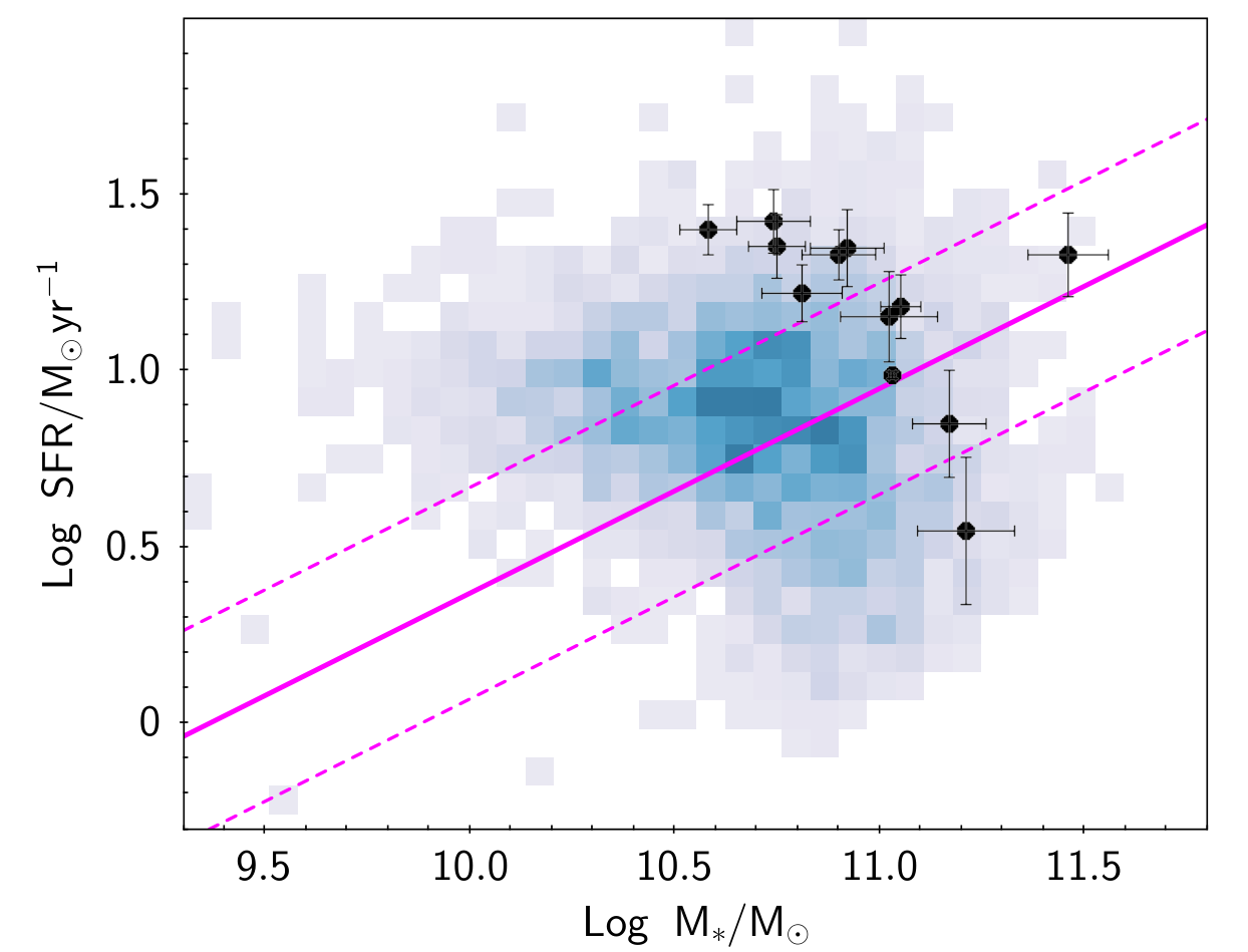
The sample has a narrow range of , making them far more ‘typical’ of galaxies at this redshift than previous very luminous IR samples (Combes et al. 2011, e.g.). The stellar masses are in the range . Comparison of the 250m selected sources with other optically selected galaxies at the same redshift from the GAMA survey (Driver et al. 2016; Baldry et al. 2018) in Figure 1 shows that the 250m selection picks out the leading edge of the optical cloud of galaxies, i.e. only the most massive or highly star forming galaxies at this redshift make it above the Herschel flux limit.
2.1 ALMA observations and data reduction
| SB name | Date | MS | p.w.v | Phase Cal. | Flux Cal. | B.P. | |||||
|---|---|---|---|---|---|---|---|---|---|---|---|
| (GHz) | (min) | (mm) | (Jy) | ||||||||
| LowV | 365.2 | 14.12.13 | X1644 | 26 | 50.2 | 0.84 | J | Pallas | J | 90 | 0.86 – 1.2 |
| 26.12.14 | X2543 | 40 | 33.3 | 0.84 | J | Ganymede | J | .. | |||
| HighV | 363.5 | 21.2.14 | X3e5 | 28 | 35.3 | 0.64 | J | Ganymede | J | 65 | 0.84 – 1.1 |
| 2.1.15 | X1e75 | 39 | 34.2 | 0.69 | J | Callisto | J | .. | |||
| 2.1.15 | X2365 | 39 | 15.4 | 0.82 | J | Ganymede | J | .. | |||
| 2.1.15 | X2606 | 39 | 34.2 | 0.91 | J | Ganymede | J | .. |
is the average rms in Jy/beam for the continuum.
Observations in the 3-mm band were made in Dec 2013 during Cycle 1 with the ALMA Band 3 receiver tuned to 85 GHz. The total integration time for all 12 sources plus calibrations was 96 minutes giving Jy per synthesised beam of . The [Ci](3P1-3P0) observations were split across Cycles 1 and 2 spanning a period from December 2013–January 2015, and using 4 tunings of the Band 7 receiver in the range 362–367 GHz. The total integration time was 10.7 hours giving Jy beam-1 with . A list of the observations is presented in Table 3.
The 3-mm Band 3 data were reduced manually using the Common Astronomy Software Applications (CASA) v4.5 package (McMullin et al. 2007) with flux calibration from Mars and the phase/bandpass calibrator J0854+2006. The two measurement sets (MS), which were observed on the same day, were concatenated before imaging having been set to a common flux scale. We created spectral line cubes using tclean in CASA in 100 channels, natural weighting was used in order to maximise signal-to-noise. We also imaged in spectral line mode, the three TDM windows which were used for the continuum at 3-mm. We did so in order to search for emission lines in the high redshift SMG discovered in our fields. The noise in these cubes was 0.4–0.5 mJy beam-1 respectively.
The Band 7 observations were set up in four Scheduling Blocks (SBs) where the sources that could share a single tuning were grouped into a given SB. Due to some of these data being taking during Cycle 2, the newer CASA v4.7 was used for the reduction. Some of the MS were calibrated using the ALMA pipeline, while others were reduced manually, depending on how the data were delivered. All MS were checked and reprocessed allowing for tailoring of the calibration to the specific issues in this data-set. For example, there are several atmospheric lines which are evident in the Band 7 data and so the pipeline calibration was modified to avoid flagging the system noise temperature ()11 1 is a representation of the noise from both receivers and the atmosphere and is used to calculate initial weightings of the visibility data. In spectral regions of high atmospheric opacity there is a resultant spike in with frequency, and as these spikes are genuine reductions in sensitivity in this part of the spectrum they should not be clipped from the calibration curves which are used in future calibrations. response in some cases, and to output the data-set from the pipeline after the generation of the water vapour radiometer (WVR) and calibration tables. The data were then manually processed from that stage so that the atmospheric lines could be flagged in the bandpass calibrator and the bandpass solutions interpolated in these regions. Additional manual flagging was also applied where required.
Imaging in B7 between 350-360 GHz was performed using the casa task tclean with a Hogbom algorithm, using natural weighting. Sources above in the dirty image were masked and lightly cleaned (to 1.5).
| EB | Typical rms | Signal-to-noise ratio of the SMG in each individual EB. | ||||||
|---|---|---|---|---|---|---|---|---|
| (Jy beam-1) | 1160.s1 | 1160.s2 | 2173 | 3366 | 4104 | 5437 | 6418 | |
| X3e5 | 136 | 5.7 | 3.4 | 3.8 | 5.5 | |||
| X1e75 | 100 | 7.9 | 8.4 | 5.3 | 4.6 | |||
| X2365 | 171 | 3.5 | 4.6 | 3.6 | 3.9 | |||
| X2606 | 170 | 4.8 | 3.1 | 3.8 | 5.5 | |||
| X1644 | 163 | 3.7 | 3.5 | 12.8 | ||||
| X2543 | 103 | 5.0 | 7.2 | 15.2 | ||||
Notes: This table records the SNR of each SMG in all of the individual Execution Blocks. In every case, there is a positive source at the same position in each EB. Sources brighter than 4 were cleaned, there is no significant change in properties with or without cleaning applied (except for the brightest source 6418, which is bright enough to self calibrate).
| Field | Number of peaks in given signal-to-noise range | ||||
|---|---|---|---|---|---|
| () | () | () | () | ||
| 1160 | 0 | 1 | 1t | 0 | 2 |
| 2173K | 0 | 0 | 1 | 0 | 1 |
| 3366K | 0 | 1 | 1 | 0 | 1 |
| 4104K | 0 | 0 | 1t | 1 | 0 |
| 5347K | 0 | 0 | 0 | 0 | 1 |
| 6418 | 0 | 0 | 0 | 0 | 1 |
Notes: Number of negative peaks more significant than compared to the positive peaks as a simple test of source robustness. There are no negative peaks at while there are 7 peaks at . A K symbol at the field name indicates that the SMG has a K-band counterpart. A t symbol indicates that this positive peak is the target low-z galaxy.
During imaging, it was obvious from the dirty images that there were point sources in the fields of at least half of the targets, which were not associated with the system. They were very obvious as they were usually much higher SNR than the target source itself. We did not run any source extraction algorithms, but merely noted when a bright point source was present in the imaging (as it needed to be cleaned) and later on went back to analyse these serendipitous detections. To check the robustness of these sources, we made two analyses. Firstly, we noted the flux and SNR of each SMG in all of the different Execution Blocks (EB) in which they were observed. Four of the SMG were observed in four execution blocks, three on the same night and another taken almost a year earlier. The other three SMG were observed in two execution blocks, taken roughly one year apart. Table 4 shows the SNR ratios for each SMG in each of the EB imaged separately. In every case, the SMG is present in each of the EB going into the final data-set. Obviously, those EB with shorter integration times, poorer weather or fewer antennae have lower SNR for the SMG, but nevertheless they are positive peaks above 3 in each of the separate observations. The resulting sample of seven robust SMG are all those detected with SNR, (in fact all of them have SNR). There are also two peaks just below the 5 threshold, which are listed as candidate sources in Table 11 but are not considered further in the analysis. The second test that we did was to count the negative and positive peaks in the final images. The results are shown in Table 5, and in no cases are any negative peaks at or below found. Furthermore, four of the SMG (with the lowest SNR) also are found to have K-band counterparts in infrared imaging from the VIKING survey (Edge et al. 2013). This combined with the detection of all SMG in all the individual EB confirms that this is a very robust set of sources. Given the number of beams in the surveyed area, we expect a false detection rate at 5 of 0.002 sources in this sample.
2.2 Flux and size measurements


We measured the fluxes of the source in two ways, firstly by fitting a Gaussian and taking the peak flux from the CASA task imfit, and secondly, by fitting a Gaussian in the plane using uvmdodelfit (Martí-Vidal et al. 2014). We used both methods as a check for systematics, and also because very little size information can be derived in the image plane for sources which are smaller than the synthesised beam. Fitting in the plane is more direct and avoids the uncertainties associated with the non-linear process of deconvolution in the imaging. The fluxes and sizes are reported in Table 6, the first row for each source lists the parameters from the fitting while the second row lists the peak flux reported by imfit (equivalent to a point source flux).
For the fitting we averaged the data across each spectral window and in intervals of 30 seconds, both of these do not lead to significant band-width or time smearing for this ALMA band. We then fixed the phase centre to be the position of the SMG and fitted with a 2D Gaussian where the flux , position, major axis size and position angle () were free parameters. The sixth parameter, the axial ratio , was found to be unconstrained by fitting, tending to an axial ratio approaching zero, usually aligned with the of the beam. This tendency produces a bias in the values for and , both of them being maximised. Since an axial ratio approaching zero is not physical, we have used a constrained fit as described in Appendix A.
The major axis source sizes fitted in this way range from 0.1–0.6′′ , and the average value of the circularised size is ′′ , which translates to kpc for . This value is comparable to other studies of SMG in which the sources were much better resolved, and so this gives a measure of confidence in our fluxes and sizes (Simpson et al. 2015; Hodge et al. 2016; Oteo et al. 2016; Rujopakarn et al. 2016; Fujimoto et al. 2017; Tadaki et al. 2017; Lang et al. 2019). The limit for reliable size determination in interferometric observations is given by Martí-Vidal et al. 2012, and using their Eqn.7 with and the 2 limit to the minimum size which could be reliably measured for our sources is listed in Table 6. Two of the sources have fit results which are comparable or slightly smaller than this limit and so for these we quote the 2 upper limit to their sizes (SDP.5347, SDP.6418). Figure 2 shows the azimuthally binned data, together with the model representing the best fit for the median likelihood axial ratio, .
There is a small difference between the peak flux derived from the fit to the imaging and the 2D fit to the data described above (where the size is a free parameter), such that the integrated fluxes from the fits with finite size are higher than the point source fluxes. This is expected, a point source flux estimate will always underestimate the flux of a source with a finite size, the degree of underestimation being dependent on the ratio of the source area compared to the beam area. To be certain that this distinction (which for the most part is not highly significant, the most significant being SDP.4104.s1 at 2.6) does not bias our subsequent study of the number counts, we checked that repeating the analysis with the peak fluxes instead of the integrated fluxes does not change the conclusions.
All fluxes and errors were then corrected for the primary beam attenuation using the primary beam model output by CASA during the clean stage. The fluxes presented in Table 6 are corrected for the primary beam, and the correction made for the primary beam attenuation is also listed there.
3 An over-density of high redshift SMG around massive galaxies at
Half of the fields observed contained one or more serendipitously detected high redshift SMG. In total 7 SMG are confidently detected at in 6 fields. The details of these SMG are given in Table 6 and images are shown in Figure 3.22 2 The ALMA images have not been corrected for the variable attenuation of the primary beam. A source nearer to the edge of the map will have a higher flux at the same signal-to-noise contour level compared to a source in the centre. This is due to the fact that the primary beam attenuation increases the noise as a function of radius from the pointing centre. We give detailed notes on each source in Appendix B.
We looked for counterparts to these SMG in VIKING K-band imaging (Edge et al. 2013; Driver et al. 2016), which is the deepest ancillary data-set in this region, and find K-band counterparts to four out of seven SMG. Counterparts or upper limits to the K-band magnitudes are noted in Table 6 and the K-band images are shown also in Figure 3.
| SMG | R.A. | Dec. | SNR | decon. size | P.B. | ||||
|---|---|---|---|---|---|---|---|---|---|
| (mJy) | ′′ | ′′ | |||||||
| 1160.s1 | 09:00:30.40 | 01:22:02.90 | 11.4 | (0.20) | 5.0 | 0.82 | |||
| 1160.s2 | 09:00:30.17 | 01:22:12.44 | 11.1 | (0.21) | 12.5 | 0.20 | |||
| 2173.s1 | 08:58:49.26 | 01:27:48.3 | 6.3 | (0.28) | 7.5 | 0.59 | |||
| 3366.s1 | 09:04:50.20 | 00:12:00.10 | 11.0 | (0.21) | 3.4 | 0.91 | |||
| 4104.s1 | 09:07:07.47 | 00:00:06.94 | 6.0 | (0.29) | 7.2 | 0.58 | |||
| 5347.s1 | 09:06:58.65 | 02:02:51.95 | 7.4 | 8.0 | 0.52 | ||||
| 6418.s1 | 09:04:02.38 | 01:07:53.4 | 23.7 | 6.0 | 0.75 | ||||
Name of SMG, R.A. and Dec., : 850m flux from two methods. First row from fitting in the plane using uvmodelfit, where the size fitted is also quoted. Second row is a minimum flux estimate, using the peak of a Gaussian fitted to the image with imfit. SNR: signal-to-noise ratio from the peak pixel and rms map noise. : Deconvolved size from the fitting (see text for details). is the minimum reliable size which can be measured given the SNR of these sources using the formalism of Martí-Vidal et al. 2012. Where the fitted size is comparable to or smaller than this size, we quote the 2 size limit in this column. : distance of the SMG to the centre of the target galaxy in arcseconds. P.B.: the primary beam correction which has been applied to these fluxes. : K-band magnitude (AB) or 3 limit at the position of the SMG using VIKING data. 1 flux measured in a 2″aperture on VIKING image created by Driver et al. 2016. 2 flux measured on VIKING image using SeXtractor to deblend the red object from the foreground and using mag auto.


3.1 Over-density calculation
In order to estimate 850m number counts from this sample, we must first sum the area observed in which a given source could have been detected with a SNR.33 3 Given that our least significant source is actually 6, going down to 5 provides a more generous area and therefore lower density estimate than if we had stated a cut off at 6.
The sensitivity of our ALMA pointings is not uniform, due to the tapering effect of the primary beam. We created a noise-map for each of the twelve fields to capture this radially varying noise level by multiplying the primary beam attenuation image by the rms noise measured in a source free region of the flux image before primary beam correction. This gives us a map of the average noise as a function of radius for each field. For the 12 noise-maps (one for each of the 12 target fields), we sum the area over which we could have detected each source at its peak measured flux at a significance level of 5 times the local noise. The surface density of a source of a given flux is then simply the inverse of this area.
There are currently only two published measures of the faint number counts at 850m using ALMA, those from Oteo et al. 2016 (henceforth O16) who used the ALMA calibrator data-set to produce a direct and unbiased measurement of the 850m counts with ALMA down to sub-mJy levels, and more recently those from Bethermin et al. 2020 (henceforth B20) who present serendipitous 850m sources detected in fields targeted at [Cii] emitters. Both of these analyses were performed in comparable ways to ours, with a selection criteria and measurement of the source fluxes using integrated 2D Gaussian fitting (although both of these works used image plane rather than () fitting).
With such small numbers, we cannot hope to make an accurate measure of the counts since our uncertainties are always going to be dominated by counting statistics. Our aim in this paper is to determine with some confidence level whether we are seeing a statistical over-density of SMG in these fields containing massive galaxies. In order to do this, we will compare our results to those of O16 and B20, exploring the impact of different criteria for the flux measurement, and the magnitude of completeness corrections. In each comparison, we utilise the results of simulations by O16 and B20, who provide completeness estimates for samples similarly selected with .
To begin with, we provide short summary of the methods used by each of the comparison counts analyses and highlight any points of difference.
O16 measure fluxes by fitting 2-D Gaussians to the image plane and using the integrated flux, although sources are detected with an initial peak pixel flux requirement . The beam-sizes are ′′ for 8 sources, and ′′ for 3 sources. Their simulations consist of point sources injected into the visibilities and recovered using their normal procedure in a uniform manner. These simulations demonstrate that completeness reaches percent at for catalogues with a 5 detection threshold (Oteo et al. 2016). This is likely to be the best case scenario as the simulated sources are all point-like while the real sources would be expected to have finite sizes (particularly in the cases with smaller synthesised beams).
B20 also measure their fluxes using integrated 2-D Gaussian fitting in the image plane, having detected the source based on a peak pixel . The beam sizes are typically ′′ . Despite having a larger beam size compared to O16 (and other studies which have measured the sizes of SMG), Bethermin et al. 2020 infer that the sources are marginally resolved by their ′′ resolution imaging, based on their finding that the ratio of the integrated flux to the peak pixel flux is significantly greater than unity. While no size measurements are explicitly mentioned in B20, we have used their Eqn.4 and Fig. 4 which relate the peak/integrated flux ratio to , to estimate the average implied deconvolved size of their sources as ′′ . The beam size for our data-set is similar to B20, and yet our plane analysis indicates that our sources have a size , with a mean of , comparable to the average size measured for SMG in the literature (′′ Lang et al. 2019 and references within). The upper range of the reported sizes in the literature is kpc (Rujopakarn et al. 2016), which translates to FWHM′′ for redshifts greater than unity. It is note-worthy that the average size of ′′ implied by the B20 analysis of the peak-to-integrated flux ratio is larger than the upper end of the range found in all of the rest of the SMG literature. This has implications for our comparison of number counts, because B20 perform their simulations of completeness including size as a variable, finding that the larger sources have much lower completeness at a given detection signal-noise ratio. In the B20 simulations, sources are injected directly into the image plane rather than into the () visibilities as in O16. As a result, the completeness corrections derived by B20 are very different at the detection threshold compared to those produced in O16 (80 percent for O16, 25–30 percent for a source with the average size of 0.72′′ implied by Fig. 4 in B20). Thus, for a given set of sources, detected and measured in identical ways the Bethermin et al. 2020 method would produce counts a factor larger than using the Oteo et al. 2016 method, solely due to the size dependence of the completeness correction, and the interpretation of the peak/integrated flux ratio as a size measurement by Bethermin et al. 2020.44 4 We note that B20 do not present any discussion of the impact of the source size on the derivation of the number counts, or the implications of their sample appearing to show such large extended sizes.
Having contrasted the methods and data-sets used we now contrast the number counts quoted by each survey. O16 use a fitting formula which describes the counts all the way from 0.4 mJy to the bright-end measured with ALMA by Simpson et al. 2015.
where , mJy, and . B20 do not fit a function to their counts but present the cumulative counts in bins, which we logarithmically interpolate to the flux values of interest to us.
The counts for the two analyses are presented in Table 7, where we are listing the ‘robust ’ counts from B20 to ensure we are not including any over-density associated with the target sources. The B20 counts are higher by a factor 1.7 -- 2.5 compared to those of O16.55 5 The errors quoted on the O16 counts are very much larger than 1/, but there is no explanation within the paper as to what other sources of error are contributing. Taking the O16 errors at face value, the B20 counts are compatible within the 1 uncertainty, but if we used a 1/ estimate for the O16 errors, then the B20 counts would be significantly higher. We must acknowledge two factors in the way the counts have been obtained which may make the B20 counts tend to be higher than those of O16. Firstly, the fields used to derive the B20 counts are targeted at high-redshift galaxies with high star formation rates. They are therefore biased sight-lines as galaxies are clustered, thus an extra signal at the same redshift might be expected. For this reason, we compare to the robust counts from B20 which will have removed any contamination from clustered sources at the same redshift as the targets. There is, however, another more subtle bias which may be present, which is in fact the topic of this paper. Magnification lensing bias means that the pre-selection of fields containing bright, high redshift objects increases the probability of sight-lines containing more large-scale structure; which weakly lenses the high redshift sources making them appear slightly brighter, and hence more likely to be selected as targets. Dusty galaxies present in any foreground structures could create a bias to higher number counts. Secondly, as mentioned earlier, the completeness corrections adopted by each study are very different, with the size-dependent completeness correction of B20 leading to much higher corrections on average for their sources compared to the point source estimates of O16.
Due to this uncertainty, we proceed to calculate our over-densities with three different assumptions about the completeness correction:
- 1.
No completeness correction applied – gives a minimum estimate of the counts for our fields.
- 2.
Completeness correction following O16 simulations, meaning our two sources with (SDP.2173, SDP.4104) have corrections of 80 percent applied to them.
- 3.
Completeness correction following B20 size dependent simulations, adopting the sizes measured for our sources using the fitting (see Table 6). This gives a completeness for SDP.2173 of 80 percent (as it is compact) but for SDP.4104, the largest source, completeness is only 35 percent.
In Table 7 we present the counts we measure with each of the three completeness scenarios. We list the over-density of sources in our survey relative to both the predicted number counts from Oteo et al. 2016, and relative to the robust () sample from B20. The minimum over-density we find when we apply no completeness correction to our counts at mJy, is 6.6–7.5 for O16 and 3–4 for B20. Furthermore, in contrast to the other studies, we have not excluded the area in the centre of the map which is covered by the target optical galaxy, which makes our surface density estimates lower limits.
Making a fairer comparison between our data and the literature, if we compare our counts using the O16 completeness correction to the O16 counts, we find an over-density of a factor 7–8. If we compare our counts using the B20 completeness correction to the B20 counts, we find over-density factors of 5–5.5.
We have estimated the 1- uncertainties on our over-density measurements using the Bayesian approach described by Kraft et al. 1991. We used the same approach to estimate the probability that we could find the observed number of sources in our fields given the null hypothesis that there is no over-density compared to the background counts. Using the O16 counts, the resulting probability rules out the null hypothesis at the 4- level; using the B20 counts the null hypothesis is ruled out at 3.6-. So, even though our over-density estimates have large uncertainties, we are confident that there is a significant over-density in our fields.
| Reference | Over-density | P(null)obs | P(null)cor | ||||||
|---|---|---|---|---|---|---|---|---|---|
| (mJy) | counts | (deg-1) | (deg-1) | (deg-1) | observed | corrected | () | () | |
| 0.82 | 7 | O16 | 25735 | 28089 | 3861 | 3.9 | 4.0 | ||
| 1.3 | 4 | 12109 | 13266 | 1609 | 3.1 | 3.2 | |||
| 0.82 | 7 | B20 | 25735 | 35529 | 6431 | 3.1 | 3.6 | ||
| 1.3 | 4 | 12109 | 20707 | 4033 | 2.1 | 2.7 | |||
Estimated counts in bins of 850m flux. is the number of sources per bin, is the surface density we measure not corrected for completeness, accounts for the completeness correction using the same method as the background counts being compared to. are the background cumulative counts from Oteo et al. 2016 (O16) and Bethermin et al. 2020 (B20) respectively. These are corrected for completeness. The over-density columns are the relative over-density in our fields (both uncorrected and corrected for completeness) compared to the literature ‘blank-field’ measures including 1 errors derived from the approach of Kraft et al. 1991. P(null) is the significance at which the null hypothesis is rejected (that the number of sources we see is a random realisation of the number counts given by the literature reference).
We next consider a possible physical explanation for this excess of SMG.
3.2 Lensing Magnification Bias
Cross-correlations between foreground structure traced by SDSS galaxies and background galaxies detected by Herschel have been detected with high significance (González-Nuevo et al. 2014; González-Nuevo et al. 2017). Anomalies in the positional offset distribution between Herschel-ATLAS sources with high-redshift submillimeter colours and foreground optical galaxies are also seen (Bourne et al. 2014). These findings both imply that there is significant magnification of the background SMG population by large scale structure in the foreground. The recent work by González-Nuevo et al. 2017(hereafter GN17) shows that lensing from the foreground halo will produce an over-density of SMG relative to the unlensed background within ′′ of halos with . The magnitude of the over-density will correlate with the distance of the SMG from the projected centre of the halo mass distribution.
We have computed the relative over-density of SMG as a function of radius from the centre (assuming that the target galaxy is the centre of its halo). Figure 4 shows our estimated cross-correlation (red dots) compared to the cross-correlation measurements obtained by GN17 (grey squares), who studied the magnification bias due to Luminous Red Galaxies with from GAMA (Baldry et al. 2018) which act as lenses on the high redshift () SMG detected by H-ATLAS. There is a good agreement between both set of measurements. To derive physical information on the typical halo that can produce such magnification bias, we perform a similar analysis to that described in Bonavera et al. 2019. By neglecting the shear effect in the magnification bias, Bonavera et al. 2019 exploit the direct relationship between the cross-correlation function and the halo convergence: , where is the slope of the integrated source counts of the background SMG sample. As is common in previous works analysing the magnification bias, we model a Navarro Frenk and White (NFW: Navarro et al. 1997) mass density profile with the mass, , and concentration, . The data do not allow a direct constraint with the current statistics, but Figure 4 shows that they are consistent with typical values of and (blue solid line). Varying each parameter by percent produces the dashed lines () and the pale blue solid lines (). There is intrinsic degeneracy between mass and concentration in the fitting, and to provide direct constraints will require a larger sample which could be split over more radial bins.
The values which are representative of the cross-correlation are in good agreement with the vs relationships from Child et al. 2018 and Dutton & Macciò 2014. The magnifications expected at for halos this massive are of the order (González-Nuevo et al. 2014) which is enough to make a substantial over-density of SMG visible due to the steep number counts in the sub-mm waveband. This halo mass corresponds to using the relationships for from both Moster et al. 2010 and Behroozi et al. 2013. We might expect to find a small group of galaxies consisting of a bright, massive central galaxy with a few additional dwarf satellites of much lower mass.

The six SMG fields have central galaxies with ; four of the six central galaxies are interacting with smaller satellites (evidence for this is the optical morphology and kinematics of CO and [Ci] , see Dunne et al. submitted for details), and a fifth (SDP.1160) is a member of a GAMA spectroscopic group with another galaxy lying outside the ALMA B7 field of view. The only galaxy for which we have no spectroscopic evidence for a close neighbour is SDP.2173, although there are three dwarf galaxies in the KIDS catalogue (de Jong et al. 2017; Cavuoti et al. 2015; Wright et al. 2018) which have located 40-90 kpc in projection and could very plausibly be in the same halo. SDP.2173 also has the brightest r-band magnitude of any of the sources we observed, . All four of the interacting systems in our sample of 12 have an SMG in the field. The GAMA survey is highly spectroscopically complete for galaxies, and groups with spectroscopic members have been catalogued in the GC3 group catalogue of Robotham & Driver 2011. While only SDP.163 and SDP.1160 are listed as group members in the GC3, our own exploration of the GAMA data cube reveals a galaxy (GAMA 372510) located a co-moving projected distance of Mpc with a from SDP.6418. Not all the galaxies with SMG in the field would be expected to be designated as groups by GAMA for two reasons. Firstly, the GAMA criteria for group identification requires sources with meeting the radius and velocity criteria. Smaller groups with one dominant bright galaxy would therefore probably not be identified as such because the second brightest group member would be fainter than the GAMA spectroscopic limit. All of our ALMA targets have , with a median for the fields containing SMG – much brighter than the typical GAMA group brightest galaxy at this redshift. Secondly inspection of the GAMA N(z) shows that the sensitivity to large scale structure drops dramatically at so the group catalogue is likely to be incomplete for intermediate mass groups at the redshifts of this sample.
The environments and optical properties of the SMG field target galaxies are listed in Table 8.
| Field | Environment | dwarf | |
|---|---|---|---|
| 1160 | GAMA group (103864) | ||
| 2173 | 3 dwarfs kpc | 0.37–0.38 | |
| 3366 | close pair | 0.26–0.38 | |
| 4104 | close pair | 0.37 | |
| 5347 | 2 dwarfs, signs of interaction | 0.62 | |
| 6418 | GAMA 372510: Mpc, | 0.42 | |
| and | |||
| also dwarf interaction |
Total absolute r-band magnitude of the galaxies in the halo. Environment: commentary on the type of environment for the target galaxy whose halo is responsible for the lensing magnification bias. Dwarf : photo-z of any dwarf satellite galaxies using KIDS data (de Jong et al. 2017; Cavuoti et al. 2015; Wright et al. 2018).
4 Boosting of the H-ATLAS fluxes by SMG in the beam.
Lensing by the halo of the massive system increases the probability of finding a high redshift SMG within the same Herschel beam as the target low redshift source. This is a proverbial can of worms for modelling statistical properties of sub-mm surveys, e.g. source counts, sub-mm colour distributions and SED modelling. Flux boosting from the SMG will affect all SPIRE fluxes, but those at longer wavelengths disproportionately so for two reasons. Firstly, the Herschel beam is larger at longer wavelengths, thus a contaminant at distance will have a higher beam profile weighting at longer wavelengths. Secondly, the sub-mm colour of the high redshift SMG will be redder (relatively brighter at 500m ) compared to the target source, as the observed frame samples closer to the peak of the SED at high redshift. The percentage contamination to the 500m flux from the high-z SMG is thus larger than that at 250m .
To estimate the contamination of the H-ATLAS fluxes for this sample at , we take the ALMA 850m flux measured for each SMG () and calculate the SPIRE fluxes the SMG should have using plausible values for the dust SED. We consider a range of redshift (), ruling out redshift ranges where the predicted 250–500m signal would be highly visible in the H-ATLAS maps at the position of the SMG. For the remaining possible redshifts we calculate , the contribution of the SMG to the Herschel m fluxes of the galaxy, by weighting the predicted SMG flux in each SPIRE band by the beam attenuation at the location of the galaxy relative to the position of the SMG:
Here refers to the SPIRE wavelength of interest in m , is the relevant beam size for SPIRE (18′′ , 25′′ and 35′′ for the 250, 350 and 500m bands). is the 850m ALMA flux of the SMG and is the redshift chosen for the prediction. The dust SED parameters we use are K and , which are plausible values for SMG (Chapman et al. 2005; da Cunha et al. 2015; Stach et al. 2019), and is the separation between the SMG and the centre of the target galaxy in arcsec.
To determine the most likely contamination values, we step through in redshift from 1.5–5 in steps of , calculating the estimated contamination signal at each redshift. We adjust the H-ATLAS catalogue fluxes for the low redshift targets (Table 2) by these contamination values and then fit the SED from UV–850m using magphys (see Section 4.2). We choose the redshift () at which the correction produces the lowest overall for the SED fit; and contamination values are listed in Table 9.66 6 The redshift and are roughly degenerate in this process but we are not attempting to constrain either; merely we wish to retrieve FIR colours which are most compatible with the PACS and ALMA 850m photometry, which we know to be uncontaminated. Interestingly, we find that the fields containing SMG with K-band counterparts produce the best fits when the SMG is assumed to be at while those without K-band counterparts have better fits when the SMG is assumed to have .
| SMG | ||||
|---|---|---|---|---|
| (mJy) | (mJy) | (mJy) | ||
| 1160.s1 | 2 | 11.0 (9.0) | 8.0 (7.1) | 3.9 (3.7) |
| 1160.s2 | 3 | 16.4 (4.6) | 18.1 (9.0) | 12.0 (8.6) |
| 1160.H1 | 4 | 17.0 (0.02) | 28.6 (0.8) | 26.0 (4.5) |
| 2173 | 1.5 | 14.4 (9.2) | 8.6 (6.7) | 3.7 (3.3) |
| 3366 | 1.5 | 13.7 (12.5) | 8.1 (7.7) | 3.5 (3.4) |
| 4104 | 2 | 19.3 (12.7) | 14.0 (11.1) | 6.9 (6.2) |
| 5347 | 4 | 3.3 (1.2) | .. (2.5) | … (2.7) |
| 6418 | 5 | 1.6 (1.2) | 4.1 (3.5) | 5.1 (4.7) |
| 6451.b7 | 4 | 1.2 (0.7) | 1.9 (1.5) | 1.8 (1.5) |
| 6451.b3 | 4 | 3.4 (0.9) | 5.7 (2.7) | 5.2 (3.6) |
is the redshift used to compute the SMG fluxes for an SED with K, and the measured flux from Table 6. Predicted flux of the SMG in the Herschel bands and in parentheses its contamination to the H-ATLAS fluxes of the galaxy. The 1160.H1 red source catalogue fluxes, 18.0, 27.7, 23.9 mJy at 250, 350, 500m Ivison et al. 2016 are replicated with an mJy SMG for our standard SED, which produces the contamination listed above. 6451.b7 is a 4.9 source in the band 7 image with a flux of mJy. 6451.b3 is a potential line emitter at 3 mm, which is given the maximum mJy based on the 3 noise at its position in the B7 image.
The boosting effect will also mean that a low redshift sub-mm source is more likely to be above the detection threshold in a flux-limited survey if its halo is acting as a lens for a SMG with small projected separation. In order to see what effect the best estimate of our boosting has on our initial sample selection, we subtract the 250m contamination in Table 9 from the flux reported in the H-ATLAS SDP catalogue from Rigby et al. 2011.77 7 This is the relevant catalogue for the purpose of this calculation since it was from here that the sample was originally selected. We then determine how many of the sources would still have been in the catalogue at had there been no SMG. There is clearly a lot of uncertainty in this rough estimate because a wide range of contaminating 250m fluxes still produce acceptable fits to both the Herschel maps and the SED fits. The two brightest sources with SMG in the field (SDP.1160 and SDP.2173) remain at for any reasonable SMG contamination estimate. Of the other four, there are possible redshift ranges where the contamination would still allow them to remain in the sample (e.g. for SDP.3366 and SDP.4104, for SDP.5347 and for SDP.6418).
Depending on the redshift of the SMG, it is entirely possibly that all six source would remain in the SDP sample even without the presence of the SMG, for the best estimate of contamination in Table 9 4/6 would remain in the sample and in the worst case, pushing the contamination to the highest permitted values only 2/6 would remain.
The possibility that the high fraction of ‘lensing’ systems in our 250m catalogue is higher than it should be due to the effect of the boosting does not negate the magnification lensing bias as an explanation for this effect, however it would need to be accounted for in the modelling to derive more accurate parameters. This is beyond the scope of this study, and much larger samples which could be selected in flux bins to mitigate this uncertainty would be required to exploit this further.
4.1 How much boosting is there for flux limited surveys with Herschel?
The sample of 12 galaxies at targeted by ALMA is a blind sample of 250m selected sources from H-ATLAS, and while small, it is an unbiased set of sources from that survey. The implications of so much boosting in the long wavelength H-ATLAS photometry could be profound. Taking the results from Tables 2& 9 we find that the average 350 (500)m boost for the fields with SMG is 1.44 (1.75). If we assume the other fields have no contamination at all then we arrive at a global average boost factor of 1.26 (1.44) at 350 (500)m . This is significantly higher than that estimated from the simulations for the H-ATLAS data release (DR1) by Valiante et al. 2016, who report an average boost of 1.09-1.1 for these flux densities in the 350 and 500m bands. At 250m the average boost is 1.23 for the SMG fields and 1.13 overall (assuming the other fields have a boost of 1.0). This agrees reasonably well with the Valiante et al. 2016 and Rigby et al. 2011 simulations indicating that the analysis of 250m data from H-ATLAS is tractable using the corrections produced in the data release papers. This boosting by lensing bias will be a redshift dependent effect because there is a higher probability for lensing events to occur for halos within a certain redshift range (dependent on the redshift distribution of the background population). For typical SMG, simulations by Lapi et al. 2012 suggest that this lensing bias will be greatest for lens halos around and will decrease sharply below . To determine the boosting corrections with more accuracy, a larger sample across a larger redshift range would be required. This effect will not be limited to the H-ATLAS survey but will affect any Herschel survey where the sources are in the redshift interval with a high probability for lensing (). The method of flux measurement is also unlikely to mitigate these boosts unless any high redshift SMG are identified at other wavelengths during source extraction using a cross-identification (XID) method (Hurley et al. 2017; Pearson et al. 2017; Wang et al. 2019, e.g.)
4.2 Impact of ALMA data on SED fits to Herschel photometry
The discovery of such a large boost to the 350m and 500m fluxes in this sample suggests that in the absence of ALMA information, SED fits to H-ATLAS (and any other non-deblended Herschel) photometry could be biased in some significant fraction of sources.
To assess this, we fitted UV-FIR SEDs for the targets to two versions of our photometry. We used the energy balance SED fitting code magphys (da Cunha et al. 2008) which uses libraries of optical and infrared SEDs with parameters drawn stochastically from physically motivated priors. We use extended infrared libraries which have an ISM cold temperature range of 10–30 K, as several of the sources favoured warmer ISM temperatures than allowed in the standard magphys infrared libraries. More details of the ancillary data used in the fitting and the full results for the sample are in Dunne et al. submitted.
In Case 1, we used H-ATLAS only data for the FIR photometry (Table 2: longest wavelength 500m ) without any adjustment for the contamination by high-z sources, i.e. what we would have done in ignorance of the 850m information from ALMA. In Case 2, we used our full FIR data-set including the ALMA 850m flux and having corrected the SPIRE 250–500m photometry for the contamination by any high-z SMG in the field as described in Section 4.
The results of the comparison are shown in Table 10, where we compute from the magphys fit as has been done in some literature studies (Hughes et al. 2017). The fits using only the Herschel photometry give (500m ) while those which additionally include the ALMA B7 data give (850m ).
The average offset in the SED-based 850m luminosity, dex (for the fields without SMG the average is 0.09 dex, while for those fields with SMG the average is 0.2 dex). The temperatures estimated for the cold dust in the diffuse ISM are sensitive to the Herschel SPIRE colours, and as expected, these are also biased in the fits to H-ATLAS only photometry in the fields with SMG. In Table 10, is the cold ISM temperature from magphys for the fits to Herschel only photometry, while are the temperatures from fits including the ALMA photometry, and having corrected the Herschel fluxes for SMG contamination. The average temperature without ALMA photometry is K (median 21.6 K), while that with ALMA 850m data and corrected fluxes is K (median 24.5 K). Part of this effect is independent of any boosting by SMG and is due to the lower signal-to-noise at the 350 and 500m wavelengths compared to 250m in the Herschel photometry. The long-wavelength ALMA flux constrains the cold dust temperature and mass, and without it we suspect that magphys fits are returning close to the median of the flat prior (20 K).
For the dust masses the bias is greater with an average offset , again the effect is much larger in fields with SMG (0.36 vs. 0.11). The effect on the derived dust mass from magphys is larger than that on because the dust mass is sensitive to temperature as well as the overall flux, and the temperatures from the Herschel only fits are lower than those which include the ALMA data.
The effect of the flux boosting on the SED fits is much smaller once ALMA data are present because the ALMA 850m data force such a tight constraint on the SED shape. Using uncorrected SPIRE fluxes in conjunction with ALMA 850m data produces differences in SED parameters which are well within the 1 errors ( dex in , dex in , dex in sSFR, and K in ). Therefore, the boosting corrections are not so important as long as the high resolution long wavelength data are present; however without ALMA data, the lack of boosting correction may lead to large biases in analyses of Herschel samples. For example, the VALES survey (Villanueva et al. 2017) was an ALMA CO(1-0) follow-up of 160m selected H-ATLAS sources in the redshift range . In one paper (Hughes et al. 2017) the H-ATLAS photometry was fitted using magphys and the SED extrapolated to give (500m ). This was then compared to the CO luminosities and calibrations for the dust-to-ISM mass factor derived. However, in a re-analysis of the literature, Dunne et al. in prep show that the average / from VALES is 0.2 dex lower than any other sample of low or high redshift sources, including this sample. We expect that this offset in / is due to the lensing magnification boosting effect shown in this work; Table 10 shows that the difference in inferred with and without the ALMA data is of this order. Other analyses potentially affected by this bias are the evolution of the 350 and 500m luminosity and dust mass functions (Dunne et al. 2011; Marchetti et al. 2016), modelling of the 350 and 500m source counts (Clements et al. 2010; Béthermin et al. 2012; Valiante et al. 2016), SED evolution (Symeonidis et al. 2013; Viero et al. 2013, e.g.) and stacking analyses (Bourne et al. 2012; Viero et al. 2013; Schreiber et al. 2015, e.g.). In particular, the stacking analyses of both Bourne et al. 2012 and Viero et al. 2013 found that the dust temperatures decreased with stellar mass in the lowest redshift bin (as we would predict based on the extra boosting at 350 and 500m due to the cosmic lensing bias). In Bourne et al. 2012, a strong increase in the stacked 500m luminosity of optically red (passive) galaxies was also seen from . A strong lensing explanation did not seem to explain those findings at that time, but the possibility of the lensing bias reported here and in González-Nuevo et al. 2014 was not known at that time. A strongly evolving optically red population which had optical spectral signatures (in stacks) of both old stellar populations and ongoing SF was found in Eales et al. 2018 using the H-ATLAS catalogues. Could these optically red sources with strongly evolving dust emission be sign-posting the halos producing the magnification lensing bias?
A larger sample of galaxies selected at 250m and imaged with ALMA will be required to understand and address these issues, and to determine the statistics of boosting due to this effect in bins of redshift and stellar mass.
The difference in SED fitted parameters when using Herschel only photometry compared to the corrected Herschel ALMA data. Name SMG 163 N 22.5 21.6 0.07 0.08 3132 N 25.9 22.4 0.19 0.15 5323† N 21.8 16.5 0.53 0.45 5526 N 24.4 25.6 6216 N 20.0 20.3 6451 N 25.0 25.7 0.03 0.06 1160 Y 28.3 21.5 0.66 0.32 2173 Y 24.5 19.7 0.40 0.26 3366 Y 26.5 20.2 0.71 0.58 4104 Y 27.7 25.4 0.22 0.06 5347 Y 19.9 20.4 0.03 0.02 6418 Y 23.4 21.7 0.14 0.001 Notes: Sources are grouped as to whether they have an SMG detected in the field at 850m . is the cold dust temperature fitted by magphys using the 850m ALMA data and making corrections for blending as described in Section 4. is the temperature fitted to the catalogued H-ATLAS photometry only with no corrections. is the difference in log between the H-ATLAS only and corrected H-ATLAS+850m photometry. is the difference in log from the best fitting magphys SED in the H-ATLAS only and corrected H-ATLAS+850m cases. † SDP.5323 has no PACS coverage and therefore its SED is very poorly constrained without the ALMA data point. We do not use this source in the analysis of average properties.
4.3 Summary of flux boosting and its implications
In summary, the 250m flux is the least affected of the SPIRE bands by the presence of a background SMG because (a) the beam size increases with increasing wavelength, and (b) the K-correction favours means that high redshift sources are relatively brighter at the longer wavelengths. The practical consequences of the contaminant sources are thus:
- •
The SMG in the Herschel beam boosts the 250m flux of the galaxy; in cases near the threshold for detection this could push the source into the H-ATLAS catalogue. This effect results in an increased probability to find a nearby background SMG for 250m sources close to the detection limit.
- •
The lensing explanation for the over-density of SMG in these fields is not weakened by the boosting effect, but the parameters derived from the modelling would be affected. This is beyond the scope of this study.
- •
The SMG in the beam reddens the Herschel sub-mm colours of the target galaxy, making them relatively brighter at 350 and 500m than they would have been without the contaminant. This mimics the effect of colder dust in the SED and leads to an underestimate of the cold dust temperature in magphys or two-component MBB fitting. For single MBB fits, it would result in a lower value for , if that were a free parameter.
- •
There are likely to be significant over-estimates of sub-mm fluxes if they are estimated by extrapolating SEDs fitted to Herschel fluxes which have been boosted in this way.
- •
The combination of flux-boosting and reddening of the SED means that and can be biased high by 0.15-0.25 dex for samples affected by this process: 350–850m sources measured with large beams.
5 Conclusions
We present serendipitous detections of high redshift dusty galaxies in ALMA 850m images of a complete sample of twelve galaxies, selected at 250m from the H-ATLAS survey.
- •
Half of the ALMA Band 7 fields contained one or more high redshift SMG, an over-density of a factor 4–6 relative to the background counts.
- •
We compared the statistics for the SMG with models of the lensing effect of group scale halos finding a remarkably good agreement, both in terms of the cross-correlation signal and the correlation between galaxies in halos with interacting satellites and the presence of SMG. Thus lensing is certainly a plausible explanation for the excess SMG detected around these sources.
- •
These extra SMG contribute significantly to the SPIRE 350 and 500m in some cases. We derive average flux-boosting factors of 1.13, 1.26 and 1.44 for the 250, 350 and 500m SPIRE bands for this group of 12 representative 250m sources at from H-ATLAS. These are significantly larger corrections at 350 and 500m than estimated by Valiante et al. 2016 who used simulations which did not include lensing between low and high-redshift sources. A boosting correction related to lensing is likely to be dependent on the redshifts of the target sources, as the probability for lensing depends on the lens-source geometry. For the lensing probability is much lower, but from it is likely that this sample is reasonably representative. Larger samples at different redshifts would be required to investigate this further.
Data Availability
The data underlying this article are publicly available from the ALMA archive http://almascience.eso.org/aq/ using the project code 2012.1.00973.S.
Acknowledgements
We thank S. Eales for helpful discussions on the impact of boosting on the H-ATLAS photometry, R. J. Ivison for healthy paranoia and an encyclopedic knowledge of SMG, and H. Gomez for careful consideration of the draft manuscript. LD and SJM acknowledge support from the European Research Council Advanced Investigator grant, COSMICISM and Consolidator grant, COSMIC DUST. LB and JGN acknowledge financial support from the PGC 2018 project PGC2018-101948-B-I00 (MICINN, FEDER) and PAPI-19-EMERG-11 (Universidad de Oviedo). JGN acknowledges financial support from the Spanish MINECO for the ‘Ramon y Cajal’ fellowship (RYC-2013-13256). This paper makes use of the following ALMA data: ADS/JAO.ALMA#2012.1.00973.S. ALMA is a partnership of ESO (representing its member states), NSF (USA) and NINS (Japan), together with NRC (Canada), MOST and ASIAA (Taiwan), and KASI (Republic of Korea), in cooperation with the Republic of Chile. The Joint ALMA Observatory is operated by ESO, AUI/NRAO and NAOJ. The National Radio Astronomy Observatory is a facility of the National Science Foundation operated under cooperative agreement by Associated Universities, Inc. The Herschel-ATLAS is a project with Herschel, which is an ESA space observatory with science instruments provided by European-led Principal Investigator consortia and with important participation from NASA. The H-ATLAS web-site is http://www.h-atlas.org. GAMA is a joint European-Australasian project based around a spectroscopic campaign using the Anglo- Australian Telescope. The GAMA input catalogue is based on data taken from the Sloan Digital Sky Survey and the UKIRT Infrared Deep Sky Survey. Complementary imaging of the GAMA regions is being obtained by a number of independent survey programs including GALEX MIS, VST KIDS, VISTA VIKING, WISE, Herschel-ATLAS, GMRT and ASKAP providing UV to radio coverage. GAMA is funded by the STFC (UK), the ARC (Australia), the AAO, and the participating institutions. The GAMA website is: http://www.gama-survey.org/. This publication has made use of data from the VIKING survey from VISTA at the ESO Paranal Observatory, programme ID 179.A-2004. Data processing has been contributed by the VISTA Data Flow System at CASU, Cambridge and WFAU, Edinburgh.
References
- ALMA Partnership et al. (2015) ALMA Partnership et al., 2015, ApJ, 808, L4
- Almaini et al. (2005) Almaini O., Dunlop J. S., Willott C. J., Alexand er D. M., Bauer F. E., Liu C. T., 2005, MNRAS, 358, 875
- Aretxaga et al. (2011) Aretxaga I., et al., 2011, MNRAS, 415, 3831
- Baldry et al. (2018) Baldry I. K., et al., 2018, MNRAS, 474, 3875
- Behroozi et al. (2013) Behroozi P. S., Wechsler R. H., Conroy C., 2013, The Astrophysical Journal, 770, 57
- Béthermin et al. (2012) Béthermin M., et al., 2012, A&A, 542, A58
- Bethermin et al. (2020) Bethermin M., et al., 2020, arXiv e-prints, p. arXiv:2002.00962
- Blain (1997) Blain A. W., 1997, MNRAS, 290, 553
- Blain et al. (1999) Blain A. W., Kneib J. P., Ivison R. J., Smail I., 1999, ApJ, 512, L87
- Bonavera et al. (2019) Bonavera L., et al., 2019, arXiv e-prints, p. arXiv:1902.03624
- Bourne et al. (2012) Bourne N., et al., 2012, MNRAS, 421, 3027
- Bourne et al. (2014) Bourne N., et al., 2014, MNRAS, 444, 1884
- Bourne et al. (2016) Bourne N., et al., 2016, MNRAS, 462, 1714
- Bussmann et al. (2015) Bussmann R. S., et al., 2015, ApJ, 812, 43
- Cañameras et al. (2015) Cañameras R., et al., 2015, A&A, 581, A105
- Cavuoti et al. (2015) Cavuoti S., et al., 2015, MNRAS, 452, 3100
- Chapman et al. (2005) Chapman S. C., Blain A. W., Smail I., Ivison R. J., 2005, ApJ, 622, 772
- Child et al. (2018) Child H. L., Habib S., Heitmann K., Frontiere N., Finkel H., Pope A., Morozov V., 2018, ApJ, 859, 55
- Clements et al. (2010) Clements D. L., et al., 2010, A&A, 518, L8
- Combes et al. (2011) Combes F., García-Burillo S., Braine J., Schinnerer E., Walter F., Colina L., 2011, A&A, 528, A124
- Cowie et al. (2002) Cowie L. L., Barger A. J., Kneib J. P., 2002, AJ, 123, 2197
- Driver et al. (2011) Driver S. P., et al., 2011, MNRAS, 413, 971
- Driver et al. (2016) Driver S. P., et al., 2016, MNRAS, 455, 3911
- Dunne et al. (2011) Dunne L., et al., 2011, MNRAS, 417, 1510
- Dutton & Macciò (2014) Dutton A. A., Macciò A. V., 2014, MNRAS, 441, 3359
- Eales et al. (2010) Eales S., et al., 2010, PASP, 122, 499
- Eales et al. (2018) Eales S., et al., 2018, MNRAS, 473, 3507
- Edge et al. (2013) Edge A., Sutherland W., Kuijken K., Driver S., McMahon R., Eales S., Emerson J. P., 2013, The Messenger, 154, 32
- Fujimoto et al. (2017) Fujimoto S., Ouchi M., Shibuya T., Nagai H., 2017, ApJ, 850, 83
- González-Nuevo et al. (2014) González-Nuevo J., et al., 2014, MNRAS, 442, 2680
- González-Nuevo et al. (2017) González-Nuevo J., et al., 2017, J. Cosmology Astropart. Phys., 2017, 024
- Graham & Liu (1995) Graham J. R., Liu M. C., 1995, ApJ, 449, L29
- Griffin et al. (2010) Griffin M. J., et al., 2010, A&A, 518, L3
- Harris et al. (2012) Harris A. I., et al., 2012, ApJ, 752, 152
- Hildebrandt et al. (2013) Hildebrandt H., et al., 2013, MNRAS, 429, 3230
- Hodge et al. (2016) Hodge J. A., et al., 2016, ApJ, 833, 103
- Hsu et al. (2016) Hsu L.-Y., Cowie L. L., Chen C.-C., Barger A. J., Wang W.-H., 2016, ApJ, 829, 25
- Hughes et al. (2017) Hughes T. M., et al., 2017, MNRAS, 468, L103
- Hurley et al. (2017) Hurley P. D., et al., 2017, MNRAS, 464, 885
- Ivison et al. (2016) Ivison R. J., et al., 2016, The Astrophysical Journal, 832, 78
- Jarugula et al. (2019) Jarugula S., et al., 2019, ApJ, 880, 92
- Knudsen et al. (2008) Knudsen K. K., van der Werf P. P., Kneib J. P., 2008, MNRAS, 384, 1611
- Kraft et al. (1991) Kraft R. P., Burrows D. N., Nousek J. A., 1991, ApJ, 374, 344
- Lang et al. (2019) Lang P., et al., 2019, ApJ, 879, 54
- Lapi et al. (2012) Lapi A., Negrello M., González-Nuevo J., Cai Z. Y., De Zotti G., Danese L., 2012, ApJ, 755, 46
- Liske et al. (2015) Liske J., et al., 2015, MNRAS, 452, 2087
- Maddox & Dunne (2020) Maddox S. J., Dunne L., 2020, MNRAS, 493, 2363
- Marchetti et al. (2016) Marchetti L., et al., 2016, MNRAS, 456, 1999
- Martí-Vidal et al. (2012) Martí-Vidal I., Pérez-Torres M. A., Lobanov A. P., 2012, A&A, 541, A135
- Martí-Vidal et al. (2014) Martí-Vidal I., Vlemmings W. H. T., Muller S., Casey S., 2014, A&A, 563, A136
- McMullin et al. (2007) McMullin J. P., Waters B., Schiebel D., Young W., Golap K., 2007, in Shaw R. A., Hill F., Bell D. J., eds, Astronomical Society of the Pacific Conference Series Vol. 376, Astronomical Data Analysis Software and Systems XVI. p. 127
- Moster et al. (2010) Moster B. P., Somerville R. S., Maulbetsch C., van den Bosch F. C., Macciò A. V., Naab T., Oser L., 2010, ApJ, 710, 903
- Navarro et al. (1997) Navarro J. F., Frenk C. S., White S. D. M., 1997, ApJ, 490, 493
- Nayyeri et al. (2017) Nayyeri H., et al., 2017, ApJ, 844, 82
- Negrello et al. (2007) Negrello M., Perrotta F., González-Nuevo J., Silva L., de Zotti G., Granato G. L., Baccigalupi C., Danese L., 2007, MNRAS, 377, 1557
- Negrello et al. (2010) Negrello M., et al., 2010, Science, 330, 800
- Negrello et al. (2017) Negrello M., et al., 2017, MNRAS, 465, 3558
- Oteo et al. (2016) Oteo I., Zwaan M. A., Ivison R. J., Smail I., Biggs A. D., 2016, ApJ, 822, 36
- Oteo et al. (2018) Oteo I., et al., 2018, ApJ, 856, 72
- Pearson et al. (2017) Pearson W. J., Wang L., van der Tak F. F. S., Hurley P. D., Burgarella D., Oliver S. J., 2017, A&A, 603, A102
- Pilbratt et al. (2010) Pilbratt G. L., et al., 2010, A&A, 518, L1
- Planck Collaboration et al. (2016) Planck Collaboration et al., 2016, A&A, 594, A13
- Poglitsch et al. (2010) Poglitsch A., et al., 2010, A&A, 518, L2
- Rigby et al. (2011) Rigby E. E., et al., 2011, MNRAS, 415, 2336
- Robotham & Driver (2011) Robotham A. S. G., Driver S. P., 2011, MNRAS, 413, 2570
- Rowan-Robinson et al. (1991) Rowan-Robinson M., et al., 1991, Nature, 351, 719
- Rujopakarn et al. (2016) Rujopakarn W., et al., 2016, ApJ, 833, 12
- Schreiber et al. (2015) Schreiber C., et al., 2015, A&A, 575, A74
- Simpson et al. (2015) Simpson J. M., et al., 2015, The Astrophysical Journal, 799, 81
- Smail et al. (1997) Smail I., Ivison R. J., Blain A. W., 1997, ApJ, 490, L5
- Smith et al. (2011) Smith D. J. B., et al., 2011, MNRAS, 416, 857
- Speagle et al. (2014) Speagle J. S., Steinhardt C. L., Capak P. L., Silverman J. D., 2014, The Astrophysical Journal Supplement Series, 214, 15
- Stach et al. (2019) Stach S. M., et al., 2019, MNRAS, 487, 4648
- Swinbank et al. (2015) Swinbank A. M., et al., 2015, ApJ, 806, L17
- Symeonidis et al. (2013) Symeonidis M., et al., 2013, MNRAS, 431, 2317
- Tadaki et al. (2017) Tadaki K.-i., et al., 2017, ApJ, 841, L25
- Valiante et al. (2016) Valiante E., et al., 2016, MNRAS, 462, 3146
- Vieira et al. (2010) Vieira J. D., et al., 2010, ApJ, 719, 763
- Viero et al. (2013) Viero M. P., et al., 2013, ApJ, 779, 32
- Villanueva et al. (2017) Villanueva V., et al., 2017, MNRAS, 470, 3775
- Wang et al. (2011) Wang L., et al., 2011, MNRAS, 414, 596
- Wang et al. (2019) Wang L., Pearson W. J., Cowley W., Trayford J. W., Béthermin M., Gruppioni C., Hurley P., Michałowski M. J., 2019, A&A, 624, A98
- Wright et al. (2016) Wright A. H., et al., 2016, MNRAS, 460, 765
- Wright et al. (2018) Wright A. H., et al., 2018, arXiv e-prints, p. arXiv:1812.06077
- Yang et al. (2019) Yang C., et al., 2019, A&A, 624, A138
- Zemcov et al. (2010) Zemcov M., Blain A., Halpern M., Levenson L., 2010, ApJ, 721, 424
- Zhang et al. (2018) Zhang Z.-Y., et al., 2018, MNRAS, 481, 59
- da Cunha et al. (2008) da Cunha E., Charlot S., Elbaz D., 2008, MNRAS, 388, 1595
- da Cunha et al. (2015) da Cunha E., et al., 2015, ApJ, 806, 110
- de Jong et al. (2017) de Jong J. T. A., et al., 2017, A&A, 604, A134
Appendix A Size fitting procedure
For the source fitting we use the CASA task uvmodelfit with a 2-d Gaussian model. The model is described by 6 parameters: the flux , position in RA and DEC, major axis size , P.A., and the axial ratio . For our data, the axial ratio is very poorly constrained and this led to a bias towards an axial ratio very close to zero, usually aligned with the P.A. of the beam. This tendency produces a bias in the value for and , both of them being pushed towards the maximum allowable values. Since an axial ratio approaching zero is not physical, we conclude that no information can be derived on the axial ratio of these sources. To avoid the bias we chose to constrain the axial ratio to physically sensible values.
If we assume that galaxies are randomly oriented disks with inclination , the distribution of will be uniform. The resulting distribution of the apparent axial ratios is non-uniform such that:
where is the intrinsic axial ratio of the disk, which is thought to be between 0.1–0.2 for disk galaxies. For a randomly oriented distribution of disks the expectation value of is 0.5, which gives . We therefore fitted the model to the data with the axial ratio fixed at and these parameters are listed in Table 6.
The range of possible unknown disk orientations will contribute to the uncertainties of the other parameters, even though we have fixed the axial ratio in the fit. The upper and lower 1- ranges of from the distribution of disk orientations are represented by the 16th and 84th percentiles () respectively. So to estimate the total uncertainties, we fit the model with fixed to its 16th and 84th percentile values, and use the resulting parameters to set the 1- upper and lower bounds on and . We then add this error in quadrature to the quoted fitting errors, to arrive at our best estimate of the uncertainties:
with a similar formalism for the other two parameters, and (which is simply the axial ratio times the major axis).
In the majority of cases, the variation of from the 16th–84th percentile range causes little extra variation in or , and so the quoted parameter is rather insensitive to the exact value of axial ratio (1–3 percent in flux and 10–20 percent for major axis). For two sources (SDP.4104, SDP.5347) there is a larger sensitivity (5–7 percent in flux and 23–62 percent in major axis), this is reflected in larger errors on the parameters.
Appendix B Notes on individual fields
SDP.1160
There are two bright SMG in this field located 5 and 12.5′′ from the optical galaxy (Fig. 3); neither have a counterpart in the VIKING K-band image (). There is also a 500m Herschel source 28.5′′ to the South that is identified in the H-ATLAS ‘red source’ catalogue, which uses a subtractive method to recover sources which are very faint at 250m but brighter at 500m (Ivison et al. 2016). The H-ATLAS red source contributes 4.5 mJy to the 500m flux for SDP.1160. This source is outside the Band 7 imaged area, but searching in the Band 3 cube we find tentative evidence for two 3-mm line sources at similar redshift at the position of the 350 and 500m peaks, see Table 11. Combining the line information with the SPIRE colours (using the red source catalogue fluxes) we find that the most plausible redshift is with the lines being either CO(4–3) or [Ci](3P1-3P0) . A very bright 850m source with a flux of 8–12 mJy would be expected in this scenario, or a number of weaker sources which together produce the red Herschel colours, such as those found by Oteo et al. 2018.
SDP.2173
SDP.3366
The galaxy is interacting with a smaller companion to the North-East, as evidenced from the [Ci] kinematics. Slightly further north we find strong 850m continuum emission from a SMG coincident with a very red source () located 3.4′′ to the north-east of the galaxy (Fig 3). There is a second, fainter, candidate SMG () just to the left of first, which is listed in Table 11 as 3366.s2. No 3-mm continuum or lines are detected at the location of the SMG.
SDP.4104
The galaxy is interacting with a similar sized companion, as evidenced by the CO and [Ci] kinematics. There is a bright SMG in this field located 7.2′′ from the largest member of the pair, which has (see Fig. 3). No 3 mm continuum or lines are detected at the location of the SMG.
SDP.5347
The galaxy is interacting with several small satellites, leaving a tidal trail of CO, [Ci] and some dust to the western side of the galaxy. There is a 850m continuum source to the north-east, which we assume to be a high redshift SMG; details are presented in Table 6 and Fig. 3. There is a faint whiff of K-band emission in a highly smoothed image, and no 3 mm continuum or line detection.
SDP.6418
The galaxy is interacting with a smaller neighbour, as evidenced by the [Ci] kinematics. The SMG in this image is strong enough for self-calibration. There is no K-band counterpart and no 3 mm or line emission detected.
SDP.6451
The SPIRE colours of this source are most definitely contaminated, as is obvious when attempting an SED fit. We searched the data-set for any evidence of sources which may be contributing to the red SPIRE colours and find two potential candidates, which are listed in Table 11. 6451.s1 is a 4.9 850m source, which is only just below the threshold we consider for calculation of the number counts. 6451l refers to a potential 3-mm line source, which just overlaps the B7 fov giving an upper limit to the 850m flux. These are not considered in the over-density calculation but listed in the Appendix for further information.
Appendix C Candidate high redshift sources.
| SMG | R.A. | Dec. | SNR | ||||
| (mJy) | (′′ ) | ||||||
| 3366.s2 | 09:04:50.31 | 00:12:00.17 | 5.1 | point | 4.2 | ||
| 4.8 | |||||||
| 6451.s1 | 09:08:50.0 | 02:26:00.85 | 4.9 | 8.7 | |||
| SMG | R.A. | Dec. | |||||
| (Jy ) | (Jy ) | (′′ ) | (GHz) | ||||
| 1160.l1 | 09:00:29.32 | 01:21:46.8 | 2.83 | 0.76 | 30 | 85.25 | |
| 1160.l2 | 09:00:28.86 | 01:21:45.1 | 0.62 | 0.12 | 30 | 85.485 | |
| 1160.l3 | 09:00:29.24 | 01:21:46.8 | 0.56 | 0.12 | 30 | 87.525 | |
| 5347.l1 | 09:06:59.22 | 02:02:20.74 | 1.73 | 0.52 | 26.9 | 85.948 | |
| 5347.l2 | 09:06:59.14 | 02:02:27.17 | 0.52 | 0.17 | 20.7 | 85.948 | |
| 6451.l1 | 09:08:48.6 | 02:26:00.8 | 1.64 | 0.37 | 13 | 99.1678 | |
| 6451.l2 | 09:08:49.3 | 02:25:59.3 | 1.95 | 0.57 | 4 | 99.509 |
Line candidates at 3-mm. There is no continuum imaging at 850m at the location of the SDP.1160 line candidates. Plausible line identifications are: CO(3–2), CO(4–3)/ [Ci](3P1-3P0) and CO(5–4), but only the solutions fit well with the SPIRE colours.