QFT treatment of a bound state in a thermal gas

In this section we discuss the relatively simple but nontrivial interacting QFT involving a single scalar field $\varphi$ subject to the Lagrangian

where the first two terms describe a free particle with mass $m$ and the last term corresponds to the quartic interaction. The coupling constant $\lambda$ is dimensionless and the theory is renormalizable [36]. For a detailed analysis of this theory in the context of perturbation theory¹¹ 1 The $\varphi^{4}$ QFT could also be trivial, in the sense that the coupling constant vanishes after the renormalization procedure is carried out, see e.g. Refs. [37, 38] and refs. therein for the discussion of this issue. see Ref. [39]. As we shall comment later on, we will introduce a non-perturbative unitarization procedure on top of Eq. (4), in such a way to make the theory finite, unitary and well defined for each value of the coupling constant $\lambda$ (even for large ones). This is done at the one-loop resummed level with a suitable subtraction constant.

In the centre of mass frame, the differential cross-section is given by [36]

where $A(s,t,u)$ is the scattering amplitude as evaluated through Feynman diagrams, and $s,t$ and $u$ are Mandelstam variables:

where $p_{1},p_{2},p_{3}$ and $p_{4}$ are four-momenta of the particles ($p_{1},p_{2}$ ingoing and $p_{3},p_{4}$ outgoing), and $\theta$ is the scattering angle. The sum of these three variables is $s+t+u=4m^{2}$. The scattering amplitude can be expressed in terms of partial waves (by keeping $s$ and $\theta$ as independent variables) as [40]:

where $P_{l}(\xi)$ with $\xi=\cos\theta$ are the Legendre polynomials with

In general, the $l$-th wave contribution to the amplitude is given by $A_{l}(s)=\frac{1}{2}\int_{-1}^{+1}d\xi A(s,\theta)P_{l}(\xi).$

In the particular case of our Lagrangian of Eq. (4), the tree-level scattering amplitude $A(s,t,u)$ takes the very simple form:

For $\lambda>0$, one has $A<0$: the (tree-level) interaction is repulsive. On the other hand for $\lambda<0$ one has $A>0,$ which corresponds to an attractive interaction. [This case implies that the vacuum $\varphi=0$ is only metastable, but this shall not affect our discussion.]

At tree-level the $s$-wave amplitude’s contribution takes the form:

while all other waves vanish, $A_{l=1,2,...}(s)=0$ (this holds true also when unitarizing the theory within the adopted resummation scheme). Further, the total cross-section reads

At threshold:

where $a_{0}^{\text{SL}}$ is the s-wave ($l=0$) scattering length (at tree-level) given by:

The factor $1/2$ in the previous equation refers to identical particles.

Next, we introduce the phase shifts. For identical particles, one has the following general definition of the $l$-th wave phase shift $\delta_{l}(s)$:

where $k=\sqrt{\frac{s}{4}-m^{2}}$ is the modulus of the three-momentum of one of the ingoing (or outgoing) particles. In the present case, the only non-vanishing phase-shift is given by $\delta_{0}(s)$

where the ‘running’ length $a_{0}(s)$ is by construction such that $a_{0}(s=4m^{2})=a_{0}^{\text{SL}}.$ Note, for $s$ just above the threshold we have

In general, the phase-shift $\delta_{0}(s)$ can be calculated as:

Next, we explore the role of $\lambda$ for the tree-level scattering. In Fig. 1 we show the behavior of phase shift $\delta_{0}(s)$ using Eq. (19) for different values of $\lambda$. For positive $\lambda$ values, the function $\delta_{0}(s)$ is negative and decreases with increasing $\sqrt{s}/m$: the slope of the curve ($\partial\delta_{0}/\partial\sqrt{s}$) is negative for any arbitrary value of $s$, which indicates an repulsive interaction. For negative $\lambda$ values, the opposite behavior is realized, signalizing attraction.

The asymptotic values $\delta_{0}(s\rightarrow\infty)$ does not tend to a multiple of $\pi,$ since the theory at first order in $\lambda$ is only unitary at that order. As a consequence, we can trust the results only when $\delta_{0}(s)$ is sufficiently small. As a related side-remark, the expression $\delta_{0}(s)=\frac{1}{2}\arcsin\left[\frac{k}{8\pi\sqrt{s}}A_{0}(s)\right]$ (which in principle follows from Eq. (17)) is also valid only when the amplitude is sufficiently small. This drawback is also due to the lack of unitarity.

All these aspects show that the unitarization is necessary, as we show in detail in the next subsection.

Here, we introduce the two-particle loop of the field $\varphi$, that we denote as $\Sigma(s).$ We start from the requirement about its imaginary part above threshold (because of the optical theorem):

We shall put here no cutoff, hence the above equation is considered valid up to arbitrary values of the variable $s$ (note, in each realistic QFT the quantity $\operatorname{Im}\Sigma(s)$ should decrease for $s$ large enough, e.g. above the GUT or the Planck scale; nevertheless, from a mathematical point of view, we can get a fully consistent treatment for any value of $s$). The loop function $\Sigma(s)$ for complex values of the variable $s$ reads

where the subtraction $C$ guarantees convergence. Here, we make the choice $\Sigma(s\rightarrow 0)=0,$ hence

This choice turns out to be very convenient for our purposes. Explicitly, the loop reads (we keep track of the arbitrary small $\epsilon$ since this will be important later on):

(For details on the $\varphi\varphi$ loops, see Ref. [41] and references therein.) For $s$ being real we get

where $\varepsilon\propto\epsilon$ is an infinitesimal positive quantity. Note. Eq. (20) is fulfilled, as it should. Moreover, for $s$ real and larger than $4m^{2}$, the real part of the loop is given by the principal part (P) of the following integral:

The function $\operatorname{Im}\Sigma(s)$ and $\operatorname{Re}\Sigma(s)$ (for real values of $s$) are presented in Fig. 2. The real part rises below threshold, has a cusp at it, then decreases monotonically and becomes negative for $\sqrt{s}/m$ large enough. The imaginary part is zero (infinitesimally small) below threshold, then it rises above it and saturates to the value $1/(32\pi)$ for large $\sqrt{s}/m$. Note, its right-hand-side derivative at threshold is infinite.

The loop function allows to calculate the unitarized amplitudes in the $k$-channel as:

All unitarized amplitudes (and consequently phase shifts) with $l=1,2,...$ vanish also at the unitarized level. The unitarized $s$-wave amplitude and phase shift are nonzero and take the form:

Hence

The scattering length is changed by the unitarization:

Within the used unitarization

hence it follows that

It is then clear that $a_{0}^{U,\text{SL}}<0$ for $\lambda>0$ (repulsion), and that $a_{0}^{U,\text{SL}}>0$ for $\lambda\in(\lambda_{c}=-16\pi^{2},0)$ (attraction). However, $a_{0}^{U,\text{SL}}<0$ for $\lambda<\lambda_{c},$ in agreement with the fact that repulsion sets in again. This is due to the fact that for $\lambda<\lambda_{c}$ a bound-state below threshold emerges, as we shall show in the next subsection.

Finally one can calculate $\delta_{0}^{U}(s)$ by using the equivalent expressions

Once the unitarization procedure is employed, the expressions (33), (34), and (28) give rise to the same result for the phase-shift. This is also a useful check of the correctness of our approach.

If $\lambda$ is negative the two scalar particles attract each other. A natural question is under which condition a bound state emerges. Such a bound state, denoted as $B$, with mass $M_{B},$ should fulfill the equation (for $s\in(0,4m^{2})$)

Since $\Sigma(s)$ is real for $s<4m^{2}$ and has a maximum at threshold with $\Sigma(s=4m^{2})=\frac{1}{16\pi^{2}}$ (see Eq. (23)), it turns out that a bound state is present if

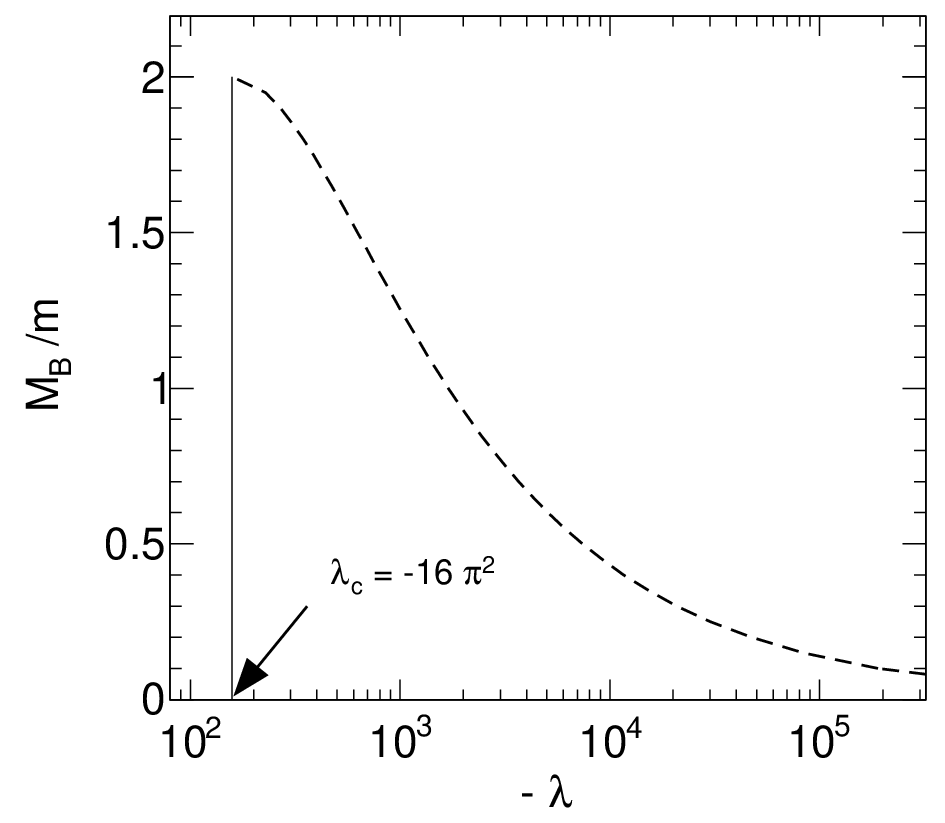
The mass $M_{B}$ as a function of $\lambda$, plotted in Fig. 3, fulfills the conditions:

This result also shows the convenience of the employed subtraction scheme: when the attraction is infinitely strong, the bound state becomes massless. This choice avoids also the emergence of an additional energy scale into the problem.

Of course, one could perform the study also for different subtraction choices: if e.g. $\Sigma(0)>0$ the mass $M_{B}$ tends to a finite value for an infinite negative coupling; if, instead, $\Sigma(0)<0$ a tachyonic mode (instability) appears for a negative coupling whose modulus is large enough. Alternatively, one could use a finite cutoff function, but this choice is linked to a non-local Lagrangian [42, 43, 44]. Yet, all these possibilities imply that a new energy scale enters into the problem. While this might be possible, that would introduce an unnecessary complication and would also spoil the fact that only the mass $m$ entering in Eq. (4) is the unique energy scale of the system.

In conclusion, the quartic theory of Eq. (4) is fully defined only once its unitarization is settled. The unitarized version of the model together with the employed subtraction constant chosen in this work assures that the model under study is well defined for any $\lambda$ (positive and negative) and is therefore very well suited for the study that we aim to do, namely the role of the bound state in a thermal bath.

In order to discuss uniterized phase shift, an important note on the adopted convention is in order. We impose that the phase-shift vanishes at threshold:

regardless on the existence of the bound state below threshold or not. In this way, the comparison between different curves is better visible. We recall that often a different convention is used, according to which the phase space at threshold equals $n_{BS}\pi,$ where $n_{BS}$ is the number of bound states below threshold [45]. Of course, the choice of the convention has no impact on the physics. For instance, the Levinson theorem [46, 47] relates the number of poles below threshold to the difference of the phase-shift at infinity and at threshold:

This quantity is clearly independent on the choice of an overall constant. In some cases, the number of poles below threshold equals the number of bound states, but care is needed, since some unphysical poles may also exist, see below.

Similarly, the finite temperature properties studied in the next section depend on the derivative $d\delta_{0}^{U}(s)/ds,$ which is also independent on the convention regarding $\delta_{0}^{U}(s=4m^{2}).$We shall also elaborate more on the behavior of $\delta_{0}^{U}(s)$ in Sec. 3.3.

Let us now present the behavior of the unitarized phase-shift $\delta_{0}^{U}(s)$ in Fig. 4. Only for small $\lambda$, the behavior of $\delta_{0}(s)$ is similar to that of Fig. 1. Yet, also in the unitarized case, for $\lambda>0$ the phase-shift and its derivative are always negative. Moreover, the asymptotic value

is realized. In addition, the point at which $\delta_{0}^{U}(s=s_{1})=-\pi/2$ is obtained for

where the amplitude becomes purely imaginary with

The point $s_{1}$ is present for each positive value of $\lambda$ since $\operatorname{Re}\Sigma(s_{1})$ is unbounded from below. According to the Levinson theorem [46, 47], Eq. (41) implies that a pole below threshold exist. Indeed, for $\lambda>0$ such a pole of the amplitude is present for a negative value of $s$ that fulfills the very same Eq. (35), but of course this pole does not correspond to a physical bound state.

Next, for $\lambda$ negative but belonging to the range $\left(\lambda_{c}=-16\pi^{2},0\right)$, the phase-shift is positive, it rises for small values of $\sqrt{s}/m,$ it reaches a maximum, and than it bends over approaching zero for large values of $s$:

This is also in agreement with the Levinson’s theorem, since no pole below threshold appears.

Finally, for $\lambda<\lambda_{c}$ the phase $\delta_{0}^{U}(s)$ is negative and approaches $-\pi$:

in accordance with Levinson’s theorem, since a pole for $s=M_{B}^{2}$ exists. Also in this case, there is a certain value $s=s_{1}$ at which the phase is $-\pi/2.$

In Fig. 5 we compare the tree level (T) and the unitarized (U) phase shifts. The top panel shows the results when $\lambda$ is small ($\pm 10$). The qualitative behavior of the phase shifts for both cases is similar for all $\sqrt{s}/m$ shown in the figure. When $\sqrt{s}/m$ is small ($<4$), the tree-level and unitarized results are very close to each other, then a discrepancy is appreciable at larger values of $\sqrt{s}/m$. In the middle panel we show a similar comparison for $\lambda=\pm 100$. In this case the unitarized phase shifts differ significantly from the tree-level ones. For $\lambda=-100$, the unitarized phase shift first increases sharply for increasing $\sqrt{s}/m$, reaches a maximum, and then starts decreasing. The magnitude of the unitarized phase shift is larger than that at tree-level at low $\sqrt{s}/m$, but becomes smaller at large $\sqrt{s}/m$. For $\lambda=+100$ both the tree level and the unitarized phase shift decrease for increasing $\sqrt{s}/m$. However, the decrease is much steeper for the unitarized phase shift. The bottom panel of Fig. 5 shows the choice $\lambda=\pm 200$. For $\lambda=200$ the comparison of the tree-level and unitarized phase shift is similar to that of $\lambda=100$. However, the behavior of unitarized phase shift for $\lambda=-200$ is completely different from the tree level one. While tree-level phase shift is positive, the unitarized phase-shift is negative because $\lambda<\lambda_{c}$. Correspondingly, in this case the bound state that dominates the near-threshold phenomenology is built.

The non-interacting part of the pressure for a gas of particles with mass $m$ reads:

In the $S$-matrix formalism [48, 49, 50, 51, 52, 53, 54, 55, 56], the interacting part of the pressure is related to the derivative of the phase shift with respect to the energy by the following relation:

where $x=\sqrt{s}$. In our specific case, only the $s$-wave contribution is nonzero:

Then, the total tree-level pressure (obviously in the absence of a bound state, since at tree-level it cannot be generated) is given by

The previous equations show that we can evaluate the pressure at $T>0$ by using solely the phase shift evaluated in the vacuum. Of course, all other relevant thermodynamic quantities of the thermal system (such as energy and entropy densities, etc.) can be determined once the pressure is known.

The temperature dependence of the corresponding pressure $(P_{\varphi,free}+P_{\varphi\varphi-int})/T^{4}$ is shown in Fig. 6. The $\lambda=0$ line corresponds to the pressure of a free gas $P_{\varphi,free}/T^{4}$ that for large $T/m$ saturates towards the massless limit ($P_{\varphi,free}/T_{m=0}^{4}=\pi^{2}/90$). For positive (negative) $\lambda$, the tree-level repulsive (attractive interaction implies that the pressure is smaller (larger) than the non-interacting case, but never exceed 0.5. As we shall see, the unitarization enhances the contribution of the interaction.

Next, in Fig. 7 we study $P_{\varphi\varphi-int}/T^{4}$ and $P_{\varphi\varphi-int}/P_{\varphi,\text{free}}$ as function of $\lambda$ for four different $m/T$ ratios $2,$ $1,$ $0.5$ and $0.2$. One can see that near $\lambda=0$, $P_{\varphi\varphi-int}/T^{4}$ changes rapidly with $\lambda$, but then saturates at large values of $\lambda$. In the right panel, one can see that all the curves of the function $P_{\varphi\varphi-int}/P_{\varphi,\text{free}}$ cross the origin at $\lambda=0,$ which is expected since there is no interaction at $\lambda=0$. Further, it can be seen that the effect of the interaction is larger both for large $\lambda$ and/or low $m/T$.

When including the unitarization procedure explained in Sec. 2.2, the interaction contribution to the pressure is obtained by using the unitarized phase-shift into the $S$-matrix formalism:

Then, the total pressure (in the absence of a bound state) is given by

Figure 8 shows the temperature dependence of pressure in the unitarized case. [Note, no bound state contribution is present here since all the considered values of the coupling $\lambda$ are larger than $\lambda_{c}$.] For small $\lambda$ ($\pm 10$), the normalized pressure saturates at large $T/m$.

Yet, for $\lambda=\pm 100$ the normalized pressure as function of the temperature is quite different from the non-interacting case, since it reaches a maximum for a finite value of the temperature. In general, this figure shows that for large values of $\lambda$ and for large temperatures, the unitarized result is sizably different from the tree level result reported in Fig. 6.

The crucial question of the present work is how to include the effect of the emergent bound state $B$ in the thermodynamics. The easiest way is to add to the pressure of the system the pressure of of mass $M_{B}$ as:

where the theta function takes into account that for $\lambda>\lambda_{c}$ there is no bound state $B.$ Of course, $M_{B}$ is itself also a function of $\lambda,$ see Eq. (35) and Fig. 3.

Within this context, the full (unitarized) pressure looks like

Quite remarkably, $P_{tot}^{U}$ turns out to be a continuous function of $\lambda$, even if $P_{B}$ is not continuous at $\lambda=\lambda_{c}$ since it jumps abruptly from $0$ to a certain finite value. Yet, the quantity $P_{\varphi\varphi\text{-int}}^{U}$ is also not continuous in such a way to compensate the previous jump, see below.

The issue is if the inclusion of $P_{B}$ as in Eq. (52) is correct. To study this point, we discuss how the contribution of the bound state can be formally included into the phase-shift analysis, showing that the simple prescription of adding one additional state to the thermodynamics is correct and the result is independent on the residuum of the pole of the bound state.

In order to show these features, let us first modify Eq. (28) by extending its validity also below the threshold. To this end we consider

where $\operatorname{Im}\Sigma(s)$ is given by Eq. (24). Clearly, above threshold nothing changes. On the other hand, below threshold we get the following expression:

Note, if $\varepsilon$ is set strictly to zero, we get obviously zero. If there is no pole below threshold, $\delta_{0}^{U}$ is an infinitesimally small number, that can be set to zero and has no effect in the description of the system.

Next, let us assume that a bound state below threshold appears: $A_{0}^{-1}(s)-\Sigma(s)=0$ for $s=M_{B}^{2}\in(0,4m^{2}).$ In this case, we have (below threshold):

where

Using the expression for the phase-shift of Eq. (34) we find:

For $0<s<M_{B}^{2}$ the argument of the $\arccos$ is $1$ (for an arbitrary small $\varepsilon$), then unitarized phase shift $\delta_{0}^{\text{U}}=n\pi,$ where $n$ is an integer. We recall that it in this work we require that $\delta_{0}^{U}(s)$ vanishes at threshold:

By assuming that there is a single pole below threshold, for $s<M_{B}^{2}$ it is useful to impose that $n=-1$:

Next, we notice that for $s=M_{B}^{2}$, the argument equals to $1-\frac{2\varepsilon^{2}}{\varepsilon^{2}}=-1,$ therefore $\delta_{0}^{U}=\frac{n}{2}\pi$ for this particular choice of $s.$

The function $\delta_{0}^{U}(s=x^{2})$ must be (for a finite $\varepsilon,$ even if arbitrarily small) a continuous and differentiable function. Hence, it follows that

Moreover, for any value of $M_{B}^{2}<s<4m^{2}$ we have

We may then conclude that for $s\in(0,4m^{2})$, alias for $x\in(0,2m)$, the phase shift takes the form:

In this way we obtain the desired result:

Quite interestingly, this result is independent on the residue of the pole $Z.$ The bound state counts always as $1,$ showing that the corresponding density of states is given by

in agreement with thermal models.

In order to understand better the behavior of the phase-shift, we show in the left panel of Fig. 9 the behavior of the unitarized phase shift below threshold for two different $\lambda$ values, one below and another above the critical value. For $\lambda=200>\lambda_{c}$, the phase shift is simply zero below the threshold and decreases with the increase of $\sqrt{s}/m$, whereas, for $\lambda=-200<\lambda_{c}$, the phase shift is $-\pi$ (according to our convention) below the mass of the bound state ($M_{B}/m\sim 1.98$). The phase shift jumps to zero for $\sqrt{s}=M_{B}$ and remains zero upto the threshold. This jump of phase shift is due to the formation of the bound state. Above threshold the phase shift decreases with the increase of $\sqrt{s}/m$.

The right panel of Fig. 9 shows the energy dependence of the derivative of the phase shift. For $\lambda=200$, the derivative of the phase shift is zero below threshold. Above threshold this quantity is negative and its magnitude increases with the increase of $\sqrt{s}/m$. For $\lambda=-200$, there is a delta function at $\sqrt{s}=M_{B}$, which is responsible for the inclusion of the bound state in the phase-shift formalism. Indeed, as shown in Eq. 50, the pressure depends on the derivative of the phase shift, hence the functions depicted in the right panel of Fig. 9 represent the two-particle energy weight.

One can also understand form the plots in Fig. 9 that, using the more common convention according to which the phase-shift equals $\pi$ at threshold when a bound state is present, would amount to consider $\delta_{0}^{U}(s)+\pi$ for $\lambda=-200$ in the left panel, while the right panel would remain unchanged. This result shows that the choice of the phase-shift value at threshold does not affect the thermodynamics (as well as any other physical property), as it should.

Finally, we turn to the thermodynamics of the system. The pressure contributions from the bound state and from the interaction can be described by the following expression

where the lower bound of the integral is now set to zero. If the bound state is present, it is automatically taken into account (independently on the binding energy).

Next, we discuss the numerical result in presence of a bound state. As we have already mentioned, the formation of bound state is possible when $\lambda$ is less than the critical value $\lambda_{c}=-16\pi^{2}$.

Figure 10 shows the temperature dependence of the normalized total pressure for $\lambda=\pm 200$. For the value $\lambda=-200$ (which is less than $\lambda_{c}$) the bound state is present and, as expected, the total normalized pressure is larger than that of non-interacting particle. For the value $\lambda=200$ the total pressure is strongly reduced. Yet, in general, the qualitative behavior of the curves for $\lambda=\pm 200$ is quite similar to those for $\lambda=\pm 100$ depicted in Fig. 8.

The left panel of Fig. 11 shows the variation of the interacting part of normalized pressure with $\lambda$ (excluding the contribution of the bound state) using the unitarized phase-shift. Unlike the tree-level result (left panel of Fig. 7), the interacting pressure in the present case is discontinuous at $\lambda=\lambda_{c}$. In fact, for $\lambda<\lambda_{c}$, the interacting part of the pressure becomes negative as a consequence of the bound state. The right panel of Fig. 11 shows the $\lambda$-dependence of interacting part of the pressure relative to that of a free gas. It shows that for $\lambda$ of the order (or larger) of $200$, the interacting part of the pressure is definitely sizable.

Figure 12 shows the behavior of the normalized total pressure as function of $\lambda$. Here, both the contribution of the bound state and of the $\varphi\varphi$ interaction above threshold are included. Quite remarkably, the total pressure is a continuous function also at $\lambda=\lambda_{c}$: the discontinuity of the interacting part of the pressure shown in the left panel of Fig. 12 is compensated by an analogous (but with opposite sign) jump of the bound state pressure.

Finally, in Fig. 13 we show the variation of $\zeta$

as function of $T/m$ for two different values of $\lambda$ for which the bound states forms: one just below the critical value, $\lambda_{c}$, and a value sizably below it, $\lambda=-200$. This ratio approaches unity when $P^{U}_{\varphi\varphi-int}$ is zero. When $\lambda$ is just below $\lambda_{c}$, this ratio is close to unity only at low $T/m$; it then decreases with the increase of $T/m$ and eventually saturates around 0.6 at higher $T/m$. So, even at high temperature $T/m$ this fraction is not negligible. Although the magnitude of $\zeta$ is smaller, the trend is similar in case of $\lambda=-200$ as well.

The results suggest that for a bound state created close to threshold (thus $\lambda$ smaller but close to $\lambda_{c}$), the bound state is indeed important, and the negative contribution to the pressure generated by the particle-particle interaction does not overcome the positive contribution of the bound state. In that case, one should better include the contribution of the bound state to the pressure, but eventually one should take into account that its quantitative role is diminished by the interaction above threshold.

References

- [1] V. T. Cocconi, T. Fazzini, G. Fidecaro, M. Legros, N. H. Lipman, and A. W. Merrison, Mass Analysis of the Secondary Particles Produced by the 25-Gev Proton Beam of the Cern Proton Synchrotron, Phys. Rev. Lett. 5 (1960) 19–21.
- [2] STAR Collaboration, B. I. Abelev et al., Observation of an Antimatter Hypernucleus, Science 328 (2010) 58–62, [arXiv:1003.2030].
- [3] STAR Collaboration, H. Agakishiev et al., Observation of the antimatter helium-4 nucleus, Nature 473 (2011) 353, [arXiv:1103.3312]. [Erratum: Nature475,412(2011)].
- [4] ALICE Collaboration, J. Adam et al., Production of light nuclei and anti-nuclei in pp and Pb-Pb collisions at energies available at the CERN Large Hadron Collider, Phys. Rev. C93 (2016), no. 2 024917, [arXiv:1506.08951].
- [5] STAR Collaboration, J. Adam et al., Measurement of the mass difference and the binding energy of the hypertriton and antihypertriton, Nature Phys. 16 (2020), no. 4 409–412, [arXiv:1904.10520].
- [6] ALICE Collaboration, S. Acharya et al., Production of (anti-)3He and (anti-)3H in p-Pb collisions at = 5.02 TeV, Phys. Rev. C101 (2020), no. 4 044906, [arXiv:1910.14401].
- [7] ALICE Collaboration, S. Acharya et al., (Anti-)Deuteron production in pp collisions at TeV, arXiv:2003.03184.
- [8] A. Esposito, A. L. Guerrieri, F. Piccinini, A. Pilloni, and A. D. Polosa, Four-Quark Hadrons: an Updated Review, Int. J. Mod. Phys. A 30 (2015) 1530002, [arXiv:1411.5997].
- [9] LHCb Collaboration, R. Aaij et al., Observation of a narrow pentaquark state, , and of two-peak structure of the , Phys. Rev. Lett. 122 (2019), no. 22 222001, [arXiv:1904.03947].
- [10] K.-J. Sun, L.-W. Chen, C. M. Ko, and Z. Xu, Probing QCD critical fluctuations from light nuclei production in relativistic heavy-ion collisions, Phys. Lett. B774 (2017) 103–107, [arXiv:1702.07620].
- [11] K.-J. Sun, L.-W. Chen, C. M. Ko, J. Pu, and Z. Xu, Light nuclei production as a probe of the QCD phase diagram, Phys. Lett. B781 (2018) 499–504, [arXiv:1801.09382].
- [12] H. Liu, D. Zhang, S. He, K.-j. Sun, N. Yu, and X. Luo, Light nuclei production in Au+Au collisions at = 5–200 GeV from JAM model, Phys. Lett. B805 (2020) 135452, [arXiv:1909.09304].
- [13] X. Luo, S. Shi, N. Xu, and Y. Zhang, A Study of the Properties of the QCD Phase Diagram in High-Energy Nuclear Collisions, Particles 3 (2020), no. 2 278–307, [arXiv:2004.00789].
- [14] K. Blum, K. C. Y. Ng, R. Sato, and M. Takimoto, Cosmic rays, antihelium, and an old navy spotlight, Phys. Rev. D96 (2017), no. 10 103021, [arXiv:1704.05431].
- [15] V. Poulin, P. Salati, I. Cholis, M. Kamionkowski, and J. Silk, Where do the AMS-02 antihelium events come from?, Phys. Rev. D99 (2019), no. 2 023016, [arXiv:1808.08961].
- [16] AMS Collaboration, V. Vagelli, Results from AMS-02 on the ISS after 6 years in space, Nuovo Cim. C42 (2019), no. 4 173.
- [17] P. J. Siemens and J. I. Kapusta, Evidence for a soft nuclear matter equation of state, Phys. Rev. Lett. 43 (1979) 1486–1489.
- [18] A. Andronic, P. Braun-Munzinger, J. Stachel, and H. Stocker, Production of light nuclei, hypernuclei and their antiparticles in relativistic nuclear collisions, Phys. Lett. B697 (2011) 203–207, [arXiv:1010.2995].
- [19] A. Andronic, P. Braun-Munzinger, K. Redlich, and J. Stachel, The statistical model in Pb-Pb collisions at the LHC, Nucl. Phys. A904-905 (2013) 535c–538c, [arXiv:1210.7724].
- [20] J. Cleymans, S. Kabana, I. Kraus, H. Oeschler, K. Redlich, and N. Sharma, Antimatter production in proton-proton and heavy-ion collisions at ultrarelativistic energies, Phys. Rev. C84 (2011) 054916, [arXiv:1105.3719].
- [21] P. G. Ortega, D. R. Entem, F. Fernandez, and E. Ruiz Arriola, Counting states and the Hadron Resonance Gas: Does X(3872) count?, Phys. Lett. B781 (2018) 678–683, [arXiv:1707.01915].
- [22] P. G. Ortega and E. Ruiz Arriola, Is X(3872) a bound state?, Chin. Phys. C 43 (2019), no. 12 124107, [arXiv:1907.01441].
- [23] H. H. Gutbrod, A. Sandoval, P. J. Johansen, A. M. Poskanzer, J. Gosset, W. G. Meyer, G. D. Westfall, and R. Stock, Final State Interactions in the Production of Hydrogen and Helium Isotopes by Relativistic Heavy Ions on Uranium, Phys. Rev. Lett. 37 (1976) 667–670.
- [24] H. Sato and K. Yazaki, On the coalescence model for high-energy nuclear reactions, Phys. Lett. 98B (1981) 153–157.
- [25] S. Mrowczynski, On the neutron proton correlations and deuteron production, Phys. Lett. B277 (1992) 43–48.
- [26] L. P. Csernai and J. I. Kapusta, Entropy and Cluster Production in Nuclear Collisions, Phys. Rept. 131 (1986) 223–318.
- [27] S. Mrowczynski, Production of light nuclei in the thermal and coalescence models, Acta Phys. Polon. B48 (2017) 707, [arXiv:1607.02267].
- [28] S. Bazak and S. Mrowczynski, vs. and production of light nuclei in relativistic heavy-ion collisions, Mod. Phys. Lett. A33 (2018), no. 25 1850142, [arXiv:1802.08212].
- [29] Z.-J. Dong, G. Chen, Q.-Y. Wang, Z.-L. She, Y.-L. Yan, F.-X. Liu, D.-M. Zhou, and B.-H. Sa, Energy dependence of light (anti)nuclei and (anti)hypertriton production in the Au-Au collision from to 5020 GeV, Eur. Phys. J. A54 (2018), no. 9 144, [arXiv:1803.01547].
- [30] K.-J. Sun and L.-W. Chen, Production of and in central Pb+Pb collisions at = 2.76 TeV within a covariant coalescence model, Phys. Rev. C94 (2016), no. 6 064908, [arXiv:1607.04037].
- [31] A. Polleri, J. P. Bondorf, and I. N. Mishustin, Effects of collective expansion on light cluster spectra in relativistic heavy ion collisions, Phys. Lett. B419 (1998) 19–24, [nucl-th/9711011].
- [32] S. Mrowczynski and P. Slon, Hadron-Deuteron Correlations and Production of Light Nuclei in Relativistic Heavy-Ion Collisions, arXiv:1904.08320.
- [33] S. Bazak and S. Mrowczynski, Production of and correlation function in relativistic heavy-ion collisions, arXiv:2001.11351.
- [34] P. Danielewicz and G. F. Bertsch, Production of deuterons and pions in a transport model of energetic heavy ion reactions, Nucl. Phys. A533 (1991) 712–748.
- [35] D. Oliinychenko, L.-G. Pang, H. Elfner, and V. Koch, Microscopic study of deuteron production in PbPb collisions at via hydrodynamics and a hadronic afterburner, Phys. Rev. C99 (2019), no. 4 044907, [arXiv:1809.03071].
- [36] M. E. Peskin and D. V. Schroeder, An Introduction to quantum field theory. Addison-Wesley, Reading, USA, 1995.
- [37] U. Wolff, Precision check on triviality of theory by a new simulation method, Phys. Rev. D 79 (2009) 105002, [arXiv:0902.3100].
- [38] A. Agodi, G. Andronico, P. Cea, M. Consoli, and L. Cosmai, The (lambda Phi**4)(4) theory on the lattice: Effective potential and triviality, Nucl. Phys. B Proc. Suppl. 63 (1998) 637–639, [hep-lat/9709057].
- [39] H. Kleinert and V. Schulte-Frohlinde, Critical properties of phi**4-theories. 2001.
- [40] A. Messiah, Quantum Mechanics. Dover Publication, New York, USA, 1999.
- [41] F. Giacosa and G. Pagliara, On the spectral functions of scalar mesons, Phys. Rev. C 76 (2007) 065204, [arXiv:0707.3594].
- [42] Y. Burdanov, G. Efimov, S. Nedelko, and S. Solunin, Meson masses within the model of induced nonlocal quark currents, Phys. Rev. D 54 (1996) 4483–4498, [hep-ph/9601344].
- [43] A. Faessler, T. Gutsche, M. Ivanov, V. E. Lyubovitskij, and P. Wang, Pion and sigma meson properties in a relativistic quark model, Phys. Rev. D 68 (2003) 014011, [hep-ph/0304031].
- [44] F. Giacosa, T. Gutsche, and A. Faessler, A Covariant constituent quark / gluon model for the glueball-quarkonia content of scalar - isoscalar mesons, Phys. Rev. C 71 (2005) 025202, [hep-ph/0408085].
- [45] J. R. E. Taylor, Scattering Theory: The Quantum Theory of Nonrelativistic Collisions. John Wiley, USA, 1972.
- [46] J. B. Hartle and C. E. Jones, Inelastic Levinson’s theorem, cdd singularities and multiple resonance poles, Annals Phys. 38 (1966) 348–362.
- [47] M. Wellner, Levinson’s Theorem (an Elementary Derivation), American Journal of Physics 32.
- [48] R. Dashen, S.-K. Ma, and H. J. Bernstein, S Matrix formulation of statistical mechanics, Phys. Rev. 187 (1969) 345–370.
- [49] R. Venugopalan and M. Prakash, Thermal properties of interacting hadrons, Nucl. Phys. A 546 (1992) 718–760.
- [50] W. Broniowski, F. Giacosa, and V. Begun, Cancellation of the meson in thermal models, Phys. Rev. C 92 (2015), no. 3 034905, [arXiv:1506.01260].
- [51] P. M. Lo, B. Friman, M. Marczenko, K. Redlich, and C. Sasaki, Repulsive interactions and their effects on the thermodynamics of a hadron gas, Phys. Rev. C 96 (2017), no. 1 015207, [arXiv:1703.00306].
- [52] P. M. Lo, S-matrix formulation of thermodynamics with N-body scatterings, Eur. Phys. J. C 77 (2017), no. 8 533, [arXiv:1707.04490].
- [53] P. M. Lo, B. Friman, K. Redlich, and C. Sasaki, S-matrix analysis of the baryon electric charge correlation, Phys. Lett. B 778 (2018) 454–458, [arXiv:1710.02711].
- [54] A. Dash, S. Samanta, and B. Mohanty, Interacting hadron resonance gas model in the K -matrix formalism, Phys. Rev. C 97 (2018), no. 5 055208, [arXiv:1802.04998].
- [55] A. Dash, S. Samanta, and B. Mohanty, Thermodynamics of a gas of hadrons with attractive and repulsive interactions within an S -matrix formalism, Phys. Rev. C 99 (2019), no. 4 044919, [arXiv:1806.02117].
- [56] P. M. Lo and F. Giacosa, Thermal contribution of unstable states, Eur. Phys. J. C 79 (2019), no. 4 336, [arXiv:1902.03203].