The Meta-Variational Quantum Eigensolver (Meta-VQE): Learning energy profiles of parameterized Hamiltonians for quantum simulation

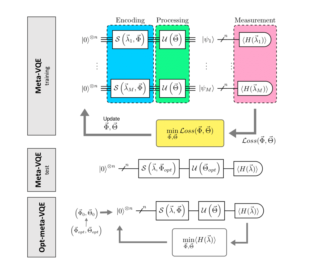
The structure of the meta-VQE is shown diagrammatically in Fig. 1. Given an $n$ qubits parametrized Hamiltonian of the form $H=H(\vec{\lambda})$, where $\vec{\lambda}=\{\lambda_{1},\lambda_{2},\cdots,\lambda_{q}\}$ are the $q$ different parameters, we select $M$ sets of $\vec{\lambda}$ that we will use as a training set. The circuit is initialized in the $|0\rangle^{\otimes n}$ state or in the Hartree-Fock state for molecules (see next section). The first part of the circuit is the encoding unitary $\mathcal{S}$ containing parametrized gates which arguments include the Hamiltonian parameters of one of the training points $\vec{\lambda}_{i}$ and variational parameters $\vec{\Phi}$. The second unitary of the circuit $\mathcal{U}$ also contains parametrized gates that depend on $\vec{\Theta}$ variables, but not the Hamiltonian parameters. The final state of the circuit can be written as

$$|\psi_{i}\rangle\equiv|\psi(\vec{\lambda}_{i},\vec{\Phi},\vec{\Theta})\rangle=\mathcal{U}(\vec{\Theta})\mathcal{S}(\vec{\lambda}_{i},\vec{\Phi})|0\rangle^{\otimes n}.$$

(1)

The meta-VQE is optimized over a set of training points $\lambda_{i}$ by minimizing a cost function that depends on all expected values of the Hamiltonians $H(\lambda_{i})$. Here we employ a simple cost function that is the sum of all expected values

$$\mathcal{L}oss(\vec{\Phi},\vec{\Theta})=\sum_{i=1}^{M}\langle\psi_{i}\lvert H(\lambda_{i})|\psi_{i}\rangle,$$

(2)

but other more sophisticated or problem-dependent ones can be developed and conveniently implemented within tequila. Finally, we minimize this loss function with a gradient-based method obtaining the optimal values for the variational parameters, $\vec{\Phi}_{opt}$ and $\vec{\Theta}_{opt}$.

Once the meta-VQE circuit is trained, we can proceed to test its performance. We compute the expected value of the Hamiltonian with other values of $\vec{\lambda}$ by running the meta-VQE circuit with the trained parameters $\vec{\Phi}_{opt}$ and $\vec{\Theta}_{opt}$ and the corresponding $\vec{\lambda}$ values for the test point. The results show that a meta-VQE is capable of learning the profile of the ground state energy as a function of the parameters $\vec{\lambda}$, but its accuracy depends strongly on the ansatz for the encoding and processing circuit. For that reason, we also propose to use the result of the meta-VQE as an initial-state guess for a standard VQE, giving what we call opt-meta-VQE. In the following subsections, we present particular examples of meta-VQE circuits and test them with different kinda of physical Hamiltonians.

Let us start with the 1D antiferromagnetic XXZ spin Hamiltonian with an external magnetic field

$$\mathcal{H}=\sum_{i=1}^{n}\sigma_{i}^{x}\sigma_{i+1}^{x}+\sigma_{i}^{y}\sigma_{i+1}^{y}+\Delta\sigma_{i}^{z}\sigma_{i+1}^{z}+\lambda\sum_{i=1}^{n}\sigma_{i}^{z},$$

(3)

where $\Delta$ is the anisotropy parameter and $\lambda$ the transverse field strength. We also consider periodic boundary conditions. For $\lambda=0$, this model contains two quantum phase transitions, at $\Delta=\pm 1$. Its ground state is a product state for $\Delta<-1$ and is highly entangled in the critical region, i.e. for $-1<\Delta\leq 1$. The introduction of the external field $\lambda$ moves the $\Delta=-1$ phase transition to higher values of $\Delta$, increasing the region with a product state as a ground state Langari 1998.

We use this model as a test for various reasons. First, this is a non-trivial model, with a highly entangled ground state, a property that motivates the use of a quantum computer. Second, there is no known quantum circuit capable of computing the ground state exactly, in contrast with other integrable models Kraus 2011; Hebenstreit et al. 2017; Schmoll and Orus 2017; Verstraete et al. 2009; Cervera-Lierta 2018; Montanaro and Stanisic 2020, although there has been recent work on the preparation of the Bethe-ansatz eigenstates using projective algorithms Van Dyke et al. 2021. Third, the energy profile as a function of $\Delta$ for a non-zero value of $\lambda$ has a non-trivial shape with a peak (see Fig. 2). Finally, some condensed matter models such as Haldane-Shastry Cirac and Sierra 2010 and some electronic Hamiltonians, are related to this model.

As stated above, no known quantum circuit represents the ground state of this model for any $n$ and $\Delta$. This gives us a good training ground to test the most general approach to a meta-VQE. We follow the same strategy as in other VQAs when applied to a general problem: we construct the quantum circuit with minimal blocks, called layers, that are concatenated and progressively introduce more variational parameters and generate entanglement. One may expect that, the greater the number of layers that are considered, the closer to the ground state the algorithm will end up. The encoding part of the meta-VQE follows a similar strategy as data re-uploading for variational quantum classification Pérez-Salinas et al. 2020: we encode the parameter $\Delta$ into rotational single-qubit gates using a linear function of the form $w\Delta+\phi$, where $w$ and $\phi$ are the variational parameters. Universality of this kind of encoding, when provided with enough layers with a single-qubit, has been shown Pérez-Salinas et al. 2020, so we expect to obtain a similar behavior when it is used on multiple qubits and entanglement is added between them. Each layer, in both the encoding and the processing part, contains first-neighbor controlled-NOT (CNOT) gates. This kind of entanglement ansatz has been proven to provide circuits with high expressibility Sim et al. 2019.

An encoding layer $l$ of the meta-VQE circuit for this model can be written in the following form

$$S_{l}\equiv S(\Delta,\vec{\Phi}_{l})=R\left(f(\Delta,\vec{\varphi}_{1l}))\otimes\cdots\otimes R(f(\Delta,\vec{\varphi}_{nl})\right)\\ \otimes CNOT\otimes\cdots\otimes CNOT,$$

(4)

where $\vec{\Phi}_{l}=(\vec{\varphi}_{1l},\cdots,\vec{\varphi}_{nl})$ and

$$R(f(\Delta,\vec{\varphi}_{il}))=R_{z}(w_{il}^{(1)}\Delta+\phi_{il}^{(1)})R_{y}(w_{il}^{(2)}\Delta+\phi_{il}^{(2)})$$

(5)

are single-qubit rotational gates with $\vec{\varphi}_{il}=(\vec{w}_{il},\vec{\phi}_{il})$, $\vec{w}_{il}=(w_{il}^{(1)},w_{il}^{(2)})$ and $\vec{\phi}_{il}=(\phi_{il}^{(1)},\phi_{il}^{(2)})$. Then, each encoding layer contains $4n$ variational parameters. Notice that this linear encoding is similar to the classical neural-network encoding, where $\vec{w}_{il}$ and $\vec{\phi}_{il}$ play the role of the weights and biases respectively, and the rotational gate plays the role of the non-linear activation function. The encoding gate is then constructed with $L_{1}$ layers:

$$\mathcal{S}(\Delta,\vec{\Phi})=S_{1}\otimes\cdots\otimes S_{L_{1}},$$

(6)

where $\vec{\Phi}=(\vec{\Phi}_{1},\cdots,\vec{\Phi}_{L_{1}})$.

Each processing layer is constructed in the same way as in Eq. (4), now with rotations that do not depend on the meta parameters. Thus, each processing layer can be written as

$$U_{l}\equiv U(\vec{\Theta}_{l})=R(\vec{\theta}_{1l})\otimes\cdots\otimes R(\vec{\theta}_{nl})\\ \otimes CNOT\otimes\cdots\otimes CNOT,$$

(7)

where

$$R(\vec{\theta}_{il})=R_{z}(\theta_{il}^{(1)})R_{y}(\theta_{il}^{(2)}).$$

(8)

Each layer of processing unitary contains $2n$ variational parameters, the components of $\vec{\theta}_{il}$. Considering $L_{2}$ processing layers, the total unitary becomes

$$\mathcal{U}(\vec{\Theta})=U_{1}\otimes\cdots\otimes U_{L_{2}},$$

(9)

with $\vec{\Theta}=(\vec{\Theta}_{1},\cdots,\vec{\Theta}_{L_{2}})$.

Figure 3 shows the circuit ansatz described above for $n=4$ qubits and two encoding and processing layers.

We run the meta-VQE for the XXZ model with a transverse field $\lambda=0.75$. The training set of $\Delta$ points is composed of 20 equispaced points between $\Delta=-1.1$ and $\Delta=1.1$. The performance of the meta-VQE is then tested through evaluation on 100 equispaced testing points between the same $\Delta$ values (and using the parameter values found after the training).

To check whether the encoding strategy of the meta-VQE entails an advantage, we run a meta-VQE with no encoding layers, i.e. all layers have the form of $U_{l}$ in Eq. (7) (a globally-averaged VQE, GA-VQE). The number of optimization parameters is then lower than the original meta-VQE, so we keep the same total number of layers to maintain the circuit depth.

To check the possible advantage of the meta-VQE learning strategy, we compare the results with those from a standard VQE. Again, we keep the total number of layers of $L_{1}+L_{2}$ and all layers are of the form of $U_{l}$ in Eq. (7). We do not consider a single-point VQE with an encoding part because the encoding function $w\Delta+\phi$ can be expressed with a single angle, $\theta$, reducing the circuit to a standard VQE. Encoding only has an effect only in the simultaneous optimization of different points. In total, the meta-VQE and opt-meta-VQE need $n(4L_{1}+2L_{2})$ variational parameters and GA-VQE and the standard VQE need $n(2L_{1}+2L_{2})$.

Finally, we check whether we can use the results of a meta-VQE and GA-VQE, that is, with and without the encoding strategy respectively, as starting points for a standard VQE (opt-meta-VQE and opt-GA-VQE). We run the simulation of a VQE again using as initial parameters the results of the meta-VQE and of the meta-VQE without encoding (GA-VQE). In both cases, the circuit depth is the same but the optimization parameters are different. The latter initializes the quantum circuit to the same state, regardless of the Hamiltonian parameter while the former provides a parameter-dependent initialization. In contrast to the standard VQE with encoding, in this case the encoding helps us to start at a specific point: if the initialization is random, the encoding can be reduced to a single rotational parameter, but if it is not, it can be used to help the algorithm to start at a particular point.

Figure 2 shows the results of these four simulations for an XXZ spin chain of 14 qubits, with two encoding and two processing layers. In all cases, the circuit is not good enough to find the ground state energy for all values of $\Delta$. The reason is simple: the circuit ansatz does not generate enough entanglement and the rotational gates are not expressible enough. This is something that we should expect since we are considering just a few layers and in turn, their design is not physically inspired. As we mentioned before, we chose this model as an example of a worst-case scenario for a VQE-type simulation, where we have no clue regarding the circuit ansatz and the initial-state preparation. The results are much better for $\Delta\lesssim 0.6$ because the ground state there corresponds to all spins being aligned with the external magnetic field (a ferromagnetic phase), i.e. in the computational basis, the state $|11\cdots 1\rangle$. This basis element is easy to find for the algorithms due to the full basis superposition induced by the $R_{y}$ gates.

It seems that a meta-VQE can find the general energy shape but not provide an accurate value, in contrast to the standard VQE. GA-VQE can reproduce only a linear profile, not learning the behavior of the energy function. However, opt-meta-VQE proves valuable, achieving better results than standard VQE with random initialization. This result is better shown in Fig. 2 right, where we plot the absolute error of all algorithms with respect to the exact solution. Whereas the standard VQE gets stuck in local minima for some values of $\Delta$, opt-meta-VQE is able to deal with those false minima and achieve better precision.

Finally, we compare the scaling of the results for different numbers of qubits and, therefore, an increasing number of optimization parameters. Figure 4 shows the relative error with respect to the exact ground state energy for the four algorithms considered for $n=8,10,12,14$. The errors decrease slightly with the number of qubits for opt-meta-VQE and opt-GA-VQE. However, the meta-VQE shows fluctuations depending on the phase of the system and the number of qubits. This behavior may be a consequence of the hardness of the optimization; we are trying to learn the ground state energy of a critical system that undergoes to a quantum phase transition with a single global cost function. The ground state will change drastically when the critical point is crossed and the encoding may be dependent on the phase. As mentioned before, we chose this model as an example of a hard-case.

To explore the role of the encoding function, we employ an example of an electronic structure problem in quantum chemistry. As before, the objective is to approximate ground-states of qubit Hamiltonians, generated in this example, by transforming second-quantized fermionic operators using various transforms Cao et al. 2019; McArdle et al. 2020. We use the $k$-UpCCGSD approach of Ref. Lee et al. 2018 in a separated form, equivalent to a single Trotter step of the full approach, as a VQE ansatz. This denotes a unitary coupled-cluster ansatz with generalized electronic single and double excitations where the double excitations are limited to electron pairs within the same spatial orbital. This ansatz is repeated $k$ times, similarly to the layered construction used before. When applied to a reference state, unitary coupled-cluster approaches are number conserving, which is a necessary condition for electronic eigenstates. In this work we use the Hartree-Fock (best product state from a classical mean-field optimization) state as a reference. In contrast to the spin Hamiltonians above the circuit construction is physically motivated illustrating a different use case of the meta-VQE approach. In the next paragraphs we give a brief description on the construction of the parametrized quantum circuit following the implementations presented in Refs. Kottmann et al. 2021; Kottmann et al. 2020.

The overall circuit consists of a collection of primitive unitary coupled-cluster operations that describe collective excitations of $n$-electrons from spin-orbitals $\mathbf{p}=(p_{0},p_{1},\dots,p_{n})$ into spin-orbitals $\mathbf{q}=(q_{0},q_{1},\dots,q_{n})$

$$U\left(\theta_{\mathbf{p}\mathbf{q}}\right)=e^{-i\frac{\theta_{\mathbf{p}\mathbf{q}}}{2}G_{\mathbf{p}\mathbf{q}}}.$$

(10)

The generators $G_{\mathbf{p}\mathbf{q}}$ are constructed from pairs of fermionic creation and annihilation operators and mapped to linear combinations of Pauli strings by various transformations with the most prominent being the Jordan-Wigner transformation which we use in this paper. In the case of $k$-UpCCGSD the types of excitation are restricted to single and double excitations where the corresponding spin-orbitals $p_{0},p_{1},q_{0},q_{1}$ are restricted to the same spatial orbital. If we index the spatial orbitals with $P$ and label the spin-up (spin-down) orbitals with even (odd) numbers, a pair restricted excitation generator in the Jordan-Wigner representation can be written as

$$G_{(2P,2P+1),(2Q,2Q+1)}\\ \xrightarrow{JW}i\left(\sigma^{+}_{2P}\sigma^{-}_{2Q}\sigma^{+}_{2P+1}\sigma^{-}_{2Q+1}-h.c.\right),$$

(11)

where $\sigma^{\pm}=\left(\sigma^{x}\pm i\sigma^{y}\right)/2$. The single excitations behave similarly but introduce additional $\sigma^{z}$ terms on intermediate qubits

$$G_{2P,2Q}\xrightarrow{JW}i\left(\sigma^{+}_{2P}\left(\prod_{k=2P+1}^{2Q-1}\sigma^{z}_{k}\right)\sigma^{-}_{2Q}-h.c.\right),$$

(12)

and analogously for $G_{2P+1,2Q+1}$. A single layer of the factorized $k$-UpCCGSD circuit is then constructed from all possible restricted double excitations and the corresponding single excitations excluding spin flips

$$U_{\text{pCCGSD}}\left(\boldsymbol{\theta}\right)=\\ \prod_{P<Q}\left(\phantom{\prod_{P,Q}}e^{-i\frac{\theta_{(2P,2Q),(2P+1,2Q+1)}}{2}G_{(2P,2Q),(2P+1,2Q+1)}}\right.\\ \left.e^{-i\frac{\theta_{2P,2Q}}{2}G_{2P,2Q}}\phantom{\prod_{P,Q}}e^{-i\frac{\theta_{2P+1,2Q+1}}{2}G_{2P+1,2Q+1}}\right),$$

(13)

with $\boldsymbol{\theta}=\left(\theta_{0213},\theta_{02},\theta_{13},\cdots,\theta_{2P,2Q,2P+1,2Q+1},\cdots\right)$, following the implementation in Ref. Kottmann et al. 2020. The full $k$-UpCCGSD circuit consists of $k$ layers with individual parameter sets acting on an initial state commonly chosen as the Hartree-Fock state

$$U\left(\boldsymbol{\theta}\right)=\prod_{k}U_{\text{pCCGSD}}\left(\boldsymbol{\theta}^{(k)}\right)U_{\text{HF}}.$$

(14)

The unitary $U_{\text{HF}}$ prepares the Hartree-Fock state which is the fermionic state with the first $N_{\text{electrons}}$ molecular spin-orbitals occupied. In the Jordan-Wigner encoding this translates to a simple computational basis state

$$U_{\text{HF}}\xrightarrow{JW}\prod_{l=0}^{{N_{\text{electrons}}}}\sigma^{x}_{l}.$$

(15)

In the standard meta-VQE approach, each UpCCGSD angle is encoded in the same way as in the previous sections using a meta parameter $d$ and a linear function,

$\displaystyle\theta_{\mathbf{p}\mathbf{q}}=w_{\mathbf{p}\mathbf{q}}\ d+\phi_{\mathbf{p}\mathbf{q}},$

(16)

with independent variational parameters $w_{\mathbf{pq}}$ and $\phi_{\mathbf{pq}}$. Additionally we introduce a non-linear encoding (nl-meta-VQE) using a single Gaussian to encode each UpCCGSD angle as

$$\theta_{\mathbf{p}\mathbf{q}}=\alpha_{\mathbf{p}\mathbf{q}}e^{\beta_{\mathbf{p}\mathbf{q}}\left(\gamma_{\mathbf{p}\mathbf{q}}-d\right)}+\delta_{\mathbf{p}\mathbf{q}},$$

(17)

with individual variational parameters $\alpha_{\mathbf{pq}}$, $\beta_{\mathbf{pq}}$, $\gamma_{\mathbf{pq}}$ and $\delta_{\mathbf{pq}}$. In comparison with the previous sections and Fig. 1 this approach contains a static (non-parametrized) initial part $U_{\text{HF}}$ and an encoded part $U_{\text{pCCGSD}}$. Note that, although it could be envisioned in future approaches, there is no processing part in the examples explored here.

In Fig. 5, we show the results of the meta-VQE with $2$-UpCCGSD applied to the dimer of two hydrogen molecules in a rectangular arrangement (see for example Ref. Lee et al. 2018) using the distance between the two molecules as a meta parameter. At 1.23Å, this results in a quadratic structure and degeneracies within the orbitals due to a change in the point-group symmetry making this point challenging for standard single-reference approaches in classical quantum chemistry.

A single layer of the UpCCGSD ansatz is not able to achieve the accuracies below the milliHartree threshold, in both absolute and relative energies, that are required for accurate chemical predictions. Using more than one layer of UpCCGSD gives enough additional freedom to the circuit, but the usual optimization strategy that initializes all angles to zero (i.e. starting from the reference state) fails to converge here and leads to no improvement from the additional layers. The meta-VQE is able to capture the basic form of the VQE results at the individual points and reaches similar accuracy as the canonical VQE at the individual points if the system is not close to the critical point.

In the original work Lee et al. 2018, repeated random initialization was used to obtain convergence to the best possible result. Here, we initialize all angles to zero for the meta-VQE as well as for the regular VQE using the BFGS optimizer of scipy with settings that worked well for previously investigated molecular systems  Kottmann et al. 2020.

We extend the meta-VQE to a non-linear encoding as given in Eq. (17), abbreviated as nl-meta-VQE, using a single Gaussian to encode each UpCCGSD angle and the intermolecular distance of the two hydrogen molecules as meta parameter $d$. The parameters are initialized such that the initial values produced are the same as for the linear meta-VQE and the canonical VQE ($\alpha,\delta=0$, $\beta,\gamma=1$). The non-linear encoding results in significantly improved convergence which can be further improved by individually optimizing the individual points with a regular VQE. Floating Gaussians are fairly good general function approximators and in this example using a single one is sufficient for the corresponding interval of interest. In addition, floating Gaussians are able to capture the asymptotic behavior of molecular distances over the constant offset $\delta$. It is expected that with increasing intermolecular distance $d$ the dependence of the UpCCGSD parameters should asymptotically approach a constant value since the system will resemble two isolated molecules. A representation with floating Gaussians automatically incorporates this property. In the same way this holds true for bond distances – see our online material for a detailed example based on a single hydrogen molecule. More general non-linear encodings are currently under investigation.

In Fig. 5 a standard VQE takes on average 3345 evaluations of the objective function, while opt-nl-meta-VQE takes 204. The training of nl-meta-VQE takes 12760 evaluations of the objective, including all five training points. The cost of obtaining a given number of test points in terms of individual expectation value estimations can then be estimated as $12760\cdot n_{\text{training-points}}+204\cdot n_{\text{test-points}}$ for the opt-nl-meta-VQE, and $3345\cdot n_{\text{test-points}}$ for the standard VQE. Since we use five training points, opt-nl-meta-VQE becomes cheaper when more than 20 test points are required. Note that those numbers should not be interpreted as rigorous benchmarks. They reflect the state of our implementation in tequila at the time of writing of manuscript. We expect, for example, further improvement by incorporating analytical gradients for unitary coupled-cluster methods Kottmann et al. 2021 in combination with an improved automatic differentiation scheme, that avoids multiple evaluations of the same objective.

As a final example, we apply the meta-VQE to a state-of-the-art application of quantum computation: the quantum computer-aided design (QCAD) of superconducting digital quantum computers Kyaw et al. 2020. We use this example to show how the meta-VQE can be applied straightforwardly to recent work.

We consider the truncated four-qubit Gray-encoded Sawaya et al. 2020 Hamiltonian for a flux-tunable transmon presented in Ref. Kyaw et al. 2020. Following the original reference, as a circuit ansatz for both the encoding and the processing layer of the meta-VQE, we consider single-qubit rotations $R_{x}$ and $R_{z}$ applied on each qubit and parameterized $XX$ gates applied to all six pairs of qubits. As a further simplification, the parameters of the $XX$ gates are common to all layers, leading to the same entangling gate after each layer of single-qubit rotations. Finally, we add a layer of $R_{x}$ and $R_{z}$ gates at the end of the processing layer. We encode linearly the Hamiltonian parameter $f$ (flux) in only the rotational gates of the encoding layers, applying the same encoding strategy as for the XXZ Hamiltonian.

In this example, we compare the meta-VQE and opt-meta-VQE with the standard VQE and improved versions of the VQE. In particular, we define VQE-smart as a standard VQE that uses as initial points the optimized points of the previous Hamiltonian parameter optimization. This approach assumes that the ground state does not change when moving drastically from close points in the Hamiltonian parameter space. We also consider the effect of the encoding layers in this kind of VQE. We define VQE-enc as a VQE that has the same parameterized quantum circuit as in the meta-VQE and in opt-meta-VQE but uses as the starting point of each minimization the optimized variables of the previous point, as in VQE-smart. The main difference between VQE-enc and opt-meta-VQE is the choice of the initialization parameters: the result of the previous optimization at each step and the result of the meta-VQE, respectively. This methodology can be further improved by running, for instance, layerwise optimization strategies Skolik et al. 2020.

The results for one encoding and one processing layer are shown in Fig. 6. The meta-VQE learns the ground-state energy with high accuracy using only 10 training points. The performance of opt-meta-VQE is better than that of the VQE, VQE-smart and VQE-enc. As one might expect, the VQE with random initialization gets stuck in local minima for some of the test points. On the other hand, VQE-smart and VQE-enc show more consistent results. The encoding strategy in VQE-enc does not prove beneficial for increasing the precision. The increase in the number of parameters to be optimized in comparison with VQE-smart can produce the emergence of local minima or barren-plateaus McClean et al. 2018, i.e. the gradients are close to zero making it difficult to explore the parameter space. However, opt-meta-VQE shows the most precise results. This fact implies that a good initialization is crucial to find the best minimum. In this case, using the initial parameters provided by the meta-VQE outperforms the initialization strategy of using the previously optimized parameters as starting point, maybe because the assumption that the ground state does not change significantly from one point to another is not accurate enough.

Besides the better performance of opt-meta-VQE, notice that for the VQE and the VQE with encoding, to obtain any point of the g.s. energy, one needs to first optimize a close point and then use the result to optimize the target point. With opt-meta-VQE this is not necessary, and any point can be obtained by using the result of the meta-VQE. The number of optimization variables involved is 30 for the VQE and 38 for the rest (the meta-VQE, opt-meta-VQE, and the VQE with encoding).

References

- Preskill (2018) J. Preskill, Quantum 2, 79 (2018).
- Bharti et al. (2021) K. Bharti, A. Cervera-Lierta, T. H. Kyaw, T. Haug, S. Alperin-Lea, A. Anand, M. Degroote, H. Heimonen, J. S. Kottmann, T. Menke, et al., arXiv:2101.08448 (2021).
- Sim et al. (2019) S. Sim, P. D. Johnson, and A. Aspuru‐Guzik, Adv. Quantum. Tech. 2, 1900070 (2019).
- Peruzzo et al. (2014) A. Peruzzo, J. McClean, P. Shadbolt, M.-H. Yung, X.-Q. Zhou, P. J. Love, A. Aspuru-Guzik, and J. L. O’Brien, Nat. Commun. 5, 4213 (2014).
- McClean et al. (2016) J. R. McClean, J. Romero, R. Babbush, and A. Aspuru-Guzik, New J. Phys. 18, 023023 (2016).
- McClean and Aspuru-Guzik (2015) J. R. McClean and A. Aspuru-Guzik, RSC Adv. 5, 102277 (2015).
- Romero et al. (2018) J. Romero, R. Babbush, J. R. McClean, C. Hempel, P. J. Love, and A. Aspuru-Guzik, Quantum Sci. Technol. 4, 014008 (2018).
- Cao et al. (2019) Y. Cao, J. Romero, J. P. Olson, M. Degroote, P. D. Johnson, M. Kieferová, I. D. Kivlichan, T. Menke, B. Peropadre, N. P. D. Sawaya, S. Sim, L. Veis, and A. Aspuru-Guzik, Chem. Rev. 119, 10856 (2019).
- Yordanov et al. (2020) Y. S. Yordanov, D. R. M. Arvidsson-Shukur, and C. H. W. Barnes, arXiv:2005.14475 (2020).
- Kraus (2011) B. Kraus, Phys. Rev. Lett. 107, 250503 (2011).
- Hebenstreit et al. (2017) M. Hebenstreit, D. Alsina, J. I. Latorre, and B. Kraus, Phys. Rev. A 95, 052339 (2017).
- Schmoll and Orus (2017) P. Schmoll and R. Orus, Phys. Rev. B 95, 045112 (2017).
- Verstraete et al. (2009) F. Verstraete, J. I. Cirac, and J. I. Latorre, Phys. Rev. A 79, 032316 (2009).
- Cervera-Lierta (2018) A. Cervera-Lierta, Quantum 2, 114 (2018).
- Montanaro and Stanisic (2020) A. Montanaro and S. Stanisic, arXiv:2006.01179 (2020).
- Farhi et al. (2014) E. Farhi, J. Goldstone, and S. Gutmann, arXiv:1411.4028 (2014).
- Lee et al. (2018) J. Lee, W. J. Huggins, M. Head-Gordon, and K. B. Whaley, J. Chem. Theory Comput. 15, 311 (2018).
- Nakaji and Yamamoto (2020) K. Nakaji and N. Yamamoto, arXiv:2005.12537 (2020).
- McClean et al. (2018) J. R. McClean, S. Boixo, V. N. Smelyanskiy, R. Babbush, and H. Neven, Nat. Commun. 9, 4812 (2018).
- Mitarai et al. (2019) K. Mitarai, T. Yan, and K. Fujii, Phys. Rev. Appl. 11, 044087 (2019).
- Cao et al. (2017) Y. Cao, G. Giacomo Guerreschi, and A. Aspuru-Guzik, arXiv:1711.11240 (2017).
- Romero et al. (2017) J. Romero, J. P. Olson, and A. Aspuru-Guzik, Quantum Sci. Technol. 2, 045001 (2017).
- Schuld and Petruccione (2018) M. Schuld and F. Petruccione, Sci Rep 8, 2772 (2018).
- Verdon et al. (2019) G. Verdon, M. Broughton, J. R. McClean, K. J. Sung, R. Babbush, Z. Jiang, H. Neven, and M. Mohseni, arXiv:1907.05415 (2019).
- Schuld et al. (2020) M. Schuld, A. Bocharov, K. Svore, and N. Wiebe, Phys. Rev. A 101, 032308 (2020).
- Pérez-Salinas et al. (2020) A. Pérez-Salinas, A. Cervera-Lierta, E. Gil-Fuster, and J. I. Latorre, Quantum 4, 226 (2020).
- Abbas et al. (2020) A. Abbas, M. Schuld, and F. Petruccione, arXiv:2001.10833 (2020).
- Zhang and Yin (2020) D.-B. Zhang and T. Yin, Phys. Rev. A 101, 032311 (2020).
- Kyaw et al. (2020) T. H. Kyaw, T. Menke, S. Sim, N. P. D. Sawaya, W. D. Oliver, G. Giacomo Guerreschi, and A. Aspuru-Guzik, arXiv:2006.03070 (2020).
- Kottmann et al. (2020) J. S. Kottmann, S. Alperin-Lea, T. Tamayo-Mendoza, A. Cervera-Lierta, C. Lavigne, T.-C. Yen, V. Verteletskyi, P. Schleich, A. Anand, M. Degroote, et al., arXiv:2011.03057 (2020).
- Suzuki et al. (2020) Y. Suzuki, Y. Kawase, Y. Masumura, Y. Hiraga, M. Nakadai, J. Chen, K. M. Nakanishi, K. Mitarai, R. Imai, S. Tamiya, et al., arXiv:2011.13524 (2020).
- Langari (1998) A. Langari, Phys. Rev. B 58, 14467 (1998).
- Van Dyke et al. (2021) J. S. Van Dyke, G. S. Barron, N. J. Mayhall, E. Barnes, and S. E. Economou, arXiv:2103.13388 (2021).
- Cirac and Sierra (2010) J. I. Cirac and G. Sierra, Phys. Rev. B 81, 104431 (2010).
- McArdle et al. (2020) S. McArdle, S. Endo, A. Aspuru-Guzik, S. C. Benjamin, and X. Yuan, Rev. Mod. Phys. 92, 015003 (2020).
- Kottmann et al. (2021) J. S. Kottmann, A. Anand, and A. Aspuru-Guzik, Chem. Sci. , (2021).
- Kottmann et al. (2020) J. S. Kottmann, P. Schleich, T. Tamayo-Mendoza, and A. Aspuru-Guzik, arXiv:2008.02819 (2020).
- Sawaya et al. (2020) N. P. D. Sawaya, T. Menke, T. H. Kyaw, S. Johri, A. Aspuru-Guzik, and G. G. Guerreschi, NPJ Quantum Inf. 6 (2020).
- Skolik et al. (2020) A. Skolik, J. R. McClean, M. Mohseni, P. van der Smagt, and M. Leib, arXiv:2006.14904 (2020).
- Cerezo et al. (2020) M. Cerezo, A. Sone, T. Volkoff, L. Cincio, and P. J. Coles, arXiv:2001.00550 [quant-ph] (2020).
- Premaratne and Matsuura (2020) S. P. Premaratne and A. Y. Matsuura, arXiv:2006.03747 (2020).
- Volkoff and Coles (2020) T. Volkoff and P. J. Coles, arXiv:2005.12200 (2020).
- Grant et al. (2019) E. Grant, L. Wossnig, M. Ostaszewski, and M. Benedetti, Quantum 3, 214 (2019).
- Wang et al. (2020) S. Wang, E. Fontana, M. Cerezo, K. Sharma, A. Sone, L. Cincio, and P. J. Coles, arXiv:2007.14384 (2020).
- Barkoutsos et al. (2018) P. K. Barkoutsos, J. F. Gonthier, I. Sokolov, N. Moll, G. Salis, A. Fuhrer, M. Ganzhorn, D. J. Egger, M. Troyer, A. Mezzacapo, S. Filipp, and I. Tavernelli, Phys. Rev. A 98, 022322 (2018).
- Cowtan et al. (2020) A. Cowtan, W. Simmons, and R. Duncan, arXiv:2007.10515 (2020).
- Fujii et al. (2020) K. Fujii, K. Mitarai, W. Mizukami, and Y. O. Nakagawa, arXiv:2007.10917 (2020).
- Huggins et al. (2020) W. J. Huggins, J. Lee, U. Baek, B. O’Gorman, and K. B. Whaley, New J. Phys. 22, 073009 (2020).
- Chivilikhin et al. (2020) D. Chivilikhin, A. Samarin, V. Ulyantsev, I. Iorsh, A. R. Oganov, and O. Kyriienko, arXiv:2007.04424 (2020).
- Endo et al. (2018) S. Endo, S. C. Benjamin, and Y. Li, Phys. Rev. X 8, 031027 (2018).