跳到论文正文
W Papers独立论文阅读器 arXiv:2009.13502 论文正文 计算阅读时间 · 0%
引用这篇论文根据当前论文元数据生成,正式投稿前建议核对。


License: arXiv.org perpetual non-exclusive license
arXiv:2009.13502v1 [math.OC] 28 Sep 2020

Simpler Grassmannian optimization

Zehua Lai Address: Computational and Applied Mathematics Initiative, University of Chicago, Chicago, IL 60637-1514. Email address: laizehua@uchicago.edu, lekheng@uchicago.edu , Lek-Heng Lim and Ke Ye Address: KLMM, Academy of Mathematics and Systems Science, Chinese Academy of Sciences, Beijing 100190, China Email address: keyk@amss.ac.cn
Abstract.

There are two widely used models for the Grassmannian Gr⁡(k,n)\Gr(k,n), as the set of equivalence classes of orthogonal matrices O⁡(n)/(O⁡(k)×O⁡(n−k))\O(n)/\bigl(\O(k)\times\O(n-k)\bigr), and as the set of trace-kk projection matrices {P∈ℝn×n:P𝖳=P=P2,tr(P)=k}\{P\in\mathbb{R}^{n\times n}:P^{\scriptscriptstyle\mathsf{T}}=P=P^{2},\;\tr(P)=k\}. The former, standard in manifold optimization, has the advantage of giving numerically stable algorithms but the disadvantage of having to work with equivalence classes of matrices. The latter, widely used in coding theory and probability, has the advantage of using actual matrices (as opposed to equivalence classes) but working with projection matrices is numerically unstable. We present an alternative that has both advantages and suffers from neither of the disadvantages; by representing kk-dimensional subspaces as symmetric orthogonal matrices of trace 2​k−n2k-n, we obtain

Gr(k,n)≅{Q∈O(n):Q𝖳=Q,tr(Q)=2k−n}.\Gr(k,n)\cong\{Q\in\O(n):Q^{\scriptscriptstyle\mathsf{T}}=Q,\;\tr(Q)=2k-n\}.

As with the other two models, we show that differential geometric objects and operations — tangent vector, metric, normal vector, exponential map, geodesic, parallel transport, gradient, Hessian, etc — have closed-form analytic expressions that are computable with standard numerical linear algebra. In the proposed model, these expressions are considerably simpler, a result of representing Gr⁡(k,n)\Gr(k,n) as a linear section of a compact matrix Lie group O⁡(n)\O(n), and can be computed with at most one qr decomposition and one exponential of a special skew-symmetric matrix that takes only O⁡(n​k​(n−k))O\bigl(nk(n-k)\bigr) time. In particular, we completely avoid eigen- and singular value decompositions in our steepest descent, conjugate gradient, quasi-Newton, and Newton methods for the Grassmannian.

Key words and phrases: 
Grassmannian, Grassmann manifold, manifold optimization
2010 Mathematics Subject Classification
14M15, 90C30, 90C53, 49Q12, 65F25, 62H12

1. Introduction

As a manifold, the Grassmannian Gr⁡(k,n)\Gr(k,n) is just the set of kk-planes in nn-space with its usual differential structure; this is an abstract description that cannot be employed in algorithms and applications. In order to optimize functions f:Gr⁡(k,n)→ℝf:\Gr(k,n)\to\mathbb{R} using currently available technology, one needs to put a coordinate system on Gr⁡(k,n)\Gr(k,n). The best known way, as discovered by Edelman, Arias, and Smith in their classic work [23], is to realize Gr⁡(k,n)\Gr(k,n) as a matrix manifold [2], where every point on Gr⁡(k,n)\Gr(k,n) is represented by a matrix or an equivalence class of matrices and from which one may derive closed-form analytic expressions for other differential geometric objects (e.g., tangent, metric, geodesic) and differential geometric operations (e.g., exponential map, parallel transport) that in turn provide the necessary ingredients (e.g., Riemannian gradient and Hessian, conjugate direction, Newton step) for optimization algorithms. The biggest advantage afforded by the approach in [23] is that a judiciously chosen system of extrinsic matrix coordinates for points on Gr⁡(k,n)\Gr(k,n) allows all aforementioned objects, operations, and algorithms to be computed solely in terms of standard numerical linear algebra, which provides a ready supply of stable and accurate algorithms [30] with high-quality software implementations [5]. In particular, one does not need to solve any differential equations numerically when doing optimization on matrix manifolds à la [23].

1.1. Existing models

There are two well-known models for Gr⁡(k,n)\Gr(k,n) supplying such matrix coordinates — one uses orthogonal matrices and the other projection matrices. In optimization, the by-now standard model (see, for example, [22, 37, 49, 54, 62]) is the one introduced in [23], namely,

(1) Gr⁡(k,n)≅O⁡(n)/(O⁡(k)×O⁡(n−k))≅V⁡(k,n)/O⁡(k),\Gr(k,n)\cong\O(n)/\bigl(\O(k)\times\O(n-k)\bigr)\cong\V(k,n)/\O(k),

where V⁡(k,n)≔{V∈ℝn×k:V𝖳​V=I}≅O⁡(n)/O⁡(n−k)\V(k,n)\coloneqq\{V\in\mathbb{R}^{n\times k}:V^{\scriptscriptstyle\mathsf{T}}V=I\}\cong\O(n)/\O(n-k) is the Stiefel manifold. In this homogeneous space model, which is also widely used in areas other than optimization [6, 7, 29, 31, 47, 48, 67], a point 𝕍∈Gr⁡(k,n)\mathbb{V}\in\Gr(k,n), i.e., a kk-dimensional subspace 𝕍⊆ℝn\mathbb{V}\subseteq\mathbb{R}^{n}, is represented by its orthonormal basis, written as columns of a matrix V=[v1,…,vk]∈V⁡(k,n)V=[v_{1},\dots,v_{k}]\in\V(k,n). Since any two orthonormal bases V1,V2∈V⁡(k,n)V_{1},V_{2}\in\V(k,n) of 𝕍\mathbb{V} must be related by V1=V2​QV_{1}=V_{2}Q for some Q∈O⁡(k)Q\in\O(k), such a representation is not unique and so this model requires that we represent 𝕍\mathbb{V} not as a single n×kn\times k orthonormal matrix but as a whole equivalence class ⟦V⟧≔{V​Q∈V⁡(k,n):Q∈O⁡(k)}\llbracket V\rrbracket\coloneqq\{VQ\in\V(k,n):Q\in\O(k)\} of orthonormal bases of 𝕍\mathbb{V}. A brief word about our notations: Throughout this article, we adopt the convention that a vector space 𝕍∈Gr⁡(k,n)\mathbb{V}\in\Gr(k,n) will be typeset in blackboard bold, with the corresponding letter in normal typeface V∈V⁡(k,n)V\in\V(k,n) denoting an (ordered) orthonormal basis. Equivalence classes will be denoted in double brackets, so ⟦V⟧=𝕍\llbracket V\rrbracket=\mathbb{V}. Diffeomorphism of two smooth manifolds will be denoted by ≅\cong.

It is straightforward to represent a point 𝕍∈Gr⁡(k,n)\mathbb{V}\in\Gr(k,n) by an actual matrix as opposed to an equivalence class of matrices. Since any subspace 𝕍\mathbb{V} has a unique orthogonal projection matrix P𝕍P_{\mathbb{V}}, this gives us an alternative model for the Grassmannian that is also widely used (notably in linear programming [55, 66] but also many other areas [14, 10, 16, 24, 46, 51]):

(2) Gr(k,n)≅{P∈ℝn×n:P𝖳=P=P2,tr(P)=k}.\Gr(k,n)\cong\{P\in\mathbb{R}^{n\times n}:P^{\scriptscriptstyle\mathsf{T}}=P=P^{2},\;\tr(P)=k\}.

Note that rank⁡(P)=tr⁡(P)=dim(𝕍)\rank(P)=\tr(P)=\dim(\mathbb{V}) for orthogonal projection matrices. The reader is reminded that an orthogonal projection matrix is not an orthogonal matrix — the ‘orthogonal’ describes the projection, not the matrix. To avoid confusion, we drop ‘orthogonal’ from future descriptions — all projection matrices in our article will be orthogonal projection matrices.

As demonstrated in [33], it is also possible to derive closed-form analytic expressions for various differential geometric objects and present various optimization algorithms in terms of the matrix coordinates in (2). Nevertheless, the problem with the model (2) is that algorithms based on projection matrices are almost always numerically unstable, especially in comparison with algorithms based on orthogonal matrices. Roughly speaking an orthogonal matrix preserves (Euclidean) norms and therefore rounding errors do not get magnified through a sequence of orthogonal transformations [20, Section 3.4.4] and consequently algorithms based on orthogonal matrices tend to be numerically stable (details are more subtle, see [63, pp. 124–166] and [35]). Projection matrices not only do not preserve norms but are singular and give notoriously unstable algorithms — possibly the best known illustration of numerical instability [60, 61] is one that contrasts Gram–Schmidt, which uses projection matrices, with Householder qr, which uses orthogonal matrices.11 1 For example, computing the qr decomposition of a Hilbert matrix A=[1/(i+j−1)]i,j=115A=[1/(i+j-1)]_{i,j=1}^{15}, we get ∥Q∗​Q−I∥≈8.0×100\lVert Q^{*}Q-I\rVert\approx 8.0\times 10^{0} with Gram–Schmidt, 1.7×1001.7\times 10^{0} with modified Gram–Schmidt, 2.4×10−152.4\times 10^{-15} with Householder qr. In fact, the proper way to compute projections is to do so via a sequence of orthogonal matrices [57, pp. 260–261], as a straightforward computation is numerically unstable [15, pp. 849–851].

The alternative (1) is currently universally adopted for optimization over a Grassmannian. The main issue with the model (1) is that a point on Gr⁡(k,n)\Gr(k,n) is not a single matrix but an equivalence class of uncountably many matrices. Equivalence classes are tricky to implement in numerical algorithms and standard algorithms in numerical linear algebra [5] do not work with equivalence classes of matrices. Indeed, any optimization algorithm [22, 23, 37, 49, 54, 62] that rely on the model (1) side steps the issue by instead optimizing an O⁡(k)\O(k)-invariant function f~:V⁡(k,n)→ℝ\tilde{f}:\V(k,n)\to\mathbb{R}, i.e., where f~​(V​Q)=f~​(V)\tilde{f}(VQ)=\tilde{f}(V) for all Q∈O⁡(k)Q\in\O(k). This practice makes it somewhat awkward to optimize over a Grassmannian: Given a function f:Gr⁡(k,n)→ℝf:\Gr(k,n)\to\mathbb{R} to be optimized, one needs to first lift it to another function f~:V⁡(k,n)→ℝ\tilde{f}:\V(k,n)\to\mathbb{R} and the choice of f~\tilde{f} is necessarily ad hoc as there are uncountably many possibilities for f~\tilde{f}. Nevertheless this is presently the only viable option.

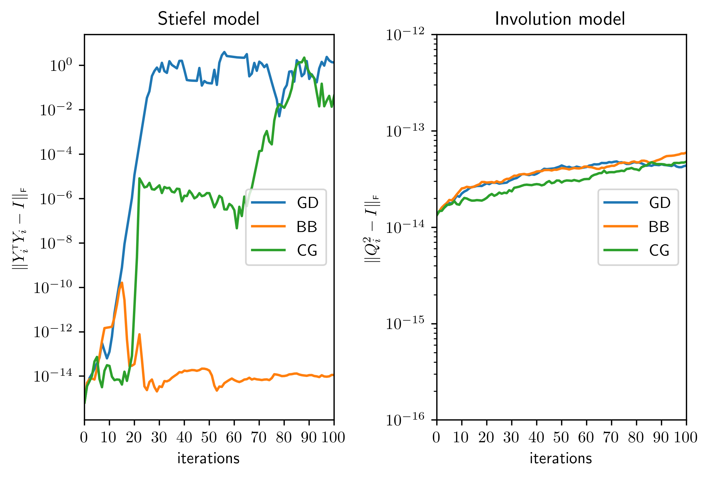
Numerical stability is of course relative, we will see in Section 8, for reasons explained therein, that the optimization algorithms in [23] for the model (1) are significantly less stable than those for our proposed model. In particular, the aforementioned loss-of-orthogonality remains very much an issue when one uses (1) to represent a Grassmannian.

We would like to mention a noncompact analogue of (1) that is popular in combinatorics [1, 25, 27, 42, 45]:

(3) Gr⁡(k,n)≅ℝkn×k/GL⁡(k),\Gr(k,n)\cong\mathbb{R}^{n\times k}_{k}/\GL(k),

with ℝkn×k≔{A∈ℝn×k:rank⁡(A)=k}\mathbb{R}^{n\times k}_{k}\coloneqq\{A\in\mathbb{R}^{n\times k}:\rank(A)=k\}. It has also been shown [2] that one may obtain closed-form analytic expressions for differential geometric quantities with the model (3) and so in principle one may use it for optimization purposes. Nevertheless, from the perspective of numerical algorithms, the model (3) suffers from the same problem as (2) — by working with rank-kk matrices, i.e., whose condition number can be arbitrarily large, algorithms based on (3) are inherently numerically unstable. In fact, since the model (3) also represents points as equivalence classes, it has both shortcomings of (1) and (2) but neither of their good features. The natural redress of imposing orthogonal constraints on (3) to get a well-conditioned representative for each equivalence class would just lead one back to the model (1).

Looking beyond optimization, we stress that each of the aforementioned models has its own (sometimes unique) strengths. For example, (3) is the only model we know in which one may naturally define the positive Grassmannian [25], an important construction in combinatorics [42] and physics [27]. The model (2) is indispensable in probability and statistics as probability measures [46, Section 3.9] and probability densities [14, Section 2.3.2] on Gr⁡(k,n)\Gr(k,n) are invariably expressed in terms of projection matrices.

1.2. Proposed model

We propose to use a model for the Grassmannian that combines the best features, suffers from none of the defects of the aforementioned models, and, somewhat surprisingly, is also simpler:

(4) Gr(k,n)≅{Q∈O(n):Q𝖳=Q,tr(Q)=2k−n}.\Gr(k,n)\cong\{Q\in\O(n):Q^{\scriptscriptstyle\mathsf{T}}=Q,\;\tr(Q)=2k-n\}.

This model, which represents kk-dimensional subspace as a symmetric orthogonal matrix of trace 2​k−n2k-n, is known but obscure. It was mentioned in passing in [9, p. 305] and was used in [39] to derive geodesics for the oriented Grassmannian, a different but related manifold. Note that (4) merely provides an expression for points, our main contribution is to derive expressions for other differential geometric objects and operations, as well as the corresponding optimization algorithms, thereby fully realizing (4) as a model for optimization. A summary of these objects, operations, and algorithms is given in Table 1. From a differential geometric perspective, Sections 2–5 may be regarded as an investigation into the embedded geometry of Gr⁡(k,n)\Gr(k,n) as a submanifold of O⁡(n)\O(n).

objects/operations results
point Proposition 2.1
change-of-coordinates Proposition 2.2, Proposition 2.3, Proposition 2.4, Proposition 2.5
tangent vector Proposition 3.1, Proposition 3.2, Corollary 3.3
metric Proposition 3.4, Proposition 3.5
normal vector Proposition 3.6, Corollary 3.7
curve Proposition 4.2
geodesic Theorem 4.3, Proposition 4.5
geodesic distance Corollary 4.6
exponential map Corollary 4.4
logarithmic map Corollary 4.7
parallel transport Proposition 4.8
gradient Proposition 5.1, Corollary 5.3
Hessian Proposition 5.2
retraction and vector transport Proposition 6.4, Proposition 6.5, Proposition 6.6
steepest descent Algorithm 1, Algorithm 2
Newton method Algorithm 3
conjugate gradient Algorithm 4
quasi-Newton Algorithm 5
Table 1. Guide to results.

The two key advantages of the model (4) in computations are immediate:

  1. (i)

    points on Gr⁡(k,n)\Gr(k,n) are represented as actual matrices, not equivalence classes;

  2. (ii)

    the matrices involved are orthogonal, so numerical stability is preserved.

The bonus with (4) is that the expressions and algorithms in Table 1 are considerably simpler compared to those in [2, 23, 33]. We will not need to solve quadratic eigenvalue problems, nor compute exp\exp/cos\cos/sin\sin/sinc\sinc of nonnormal matrices, nor even evd or svd except in cases when they can be trivially obtained. Aside from standard matrix arithmetic, our optimization algorithms require just two operations:

  1. (iii)

    all differential geometric objects and operations can be computed with at most a qr decomposition and an exponentiation of a skew-symmetric matrix,

    exp⁡([0B−B𝖳0]),B∈ℝk×(n−k),\exp\biggl(\begin{bmatrix}0&B\\ -B^{\scriptscriptstyle\mathsf{T}}&0\end{bmatrix}\biggr),\quad B\in\mathbb{R}^{k\times(n-k)},

    which may in turn be computed in time O⁡(n​k​(n−k))O\bigl(nk(n-k)\bigr) with a specialized algorithm based on Strang splitting.

The problem of computing matrix exponential has been thoroughly studied and there is a plethora of algorithms [36, 50], certainly more so than other transcendental matrix functions like cosine, sine, or sinc [36]. For normal matrices, matrix exponentiation is a well-conditioned problem — the numerical issues described in [50] only occur with nonnormal matrices. For us, [0B−B𝖳0]\begin{bmatrix}0&B\\ \smash[b]{-B^{\scriptscriptstyle\mathsf{T}}}&0\end{bmatrix} is skew-symmetric and thus normal; in fact its exponential will always be an orthogonal matrix.

There are other algorithmic advantages afforded by (4) that are difficult to explain without context and will be discussed alongside the algorithms in Section 7 and numerical results in Section 8.

1.3. Nomenclatures and notations

For easy reference, we will introduce names for the models (1)–(4) based on the type of matrices used as coordinates for points.

name model coordinates for a point
orthogonal model O⁡(n)/(O⁡(k)×O⁡(n−k))\O(n)/\bigl(\O(k)\times\O(n-k)\bigr) equivalence class of n×nn\times n orthogonal matrices ⟦V⟧\llbracket V\rrbracket
Stiefel model V⁡(k,n)/O⁡(k)\V(k,n)/\O(k) equivalence class of n×kn\times k orthonormal matrices ⟦Y⟧\llbracket Y\rrbracket
full-rank model ℝkn×k/GL⁡(k)\mathbb{R}^{n\times k}_{k}/\GL(k) equivalence class of n×kn\times k full-rank matrices ⟦A⟧\llbracket A\rrbracket
projection model {P∈ℝn×n:P𝖳=P=P2,tr(P)=k}\{P\in\mathbb{R}^{n\times n}:P^{\scriptscriptstyle\mathsf{T}}=P=P^{2},\;\tr(P)=k\} n×nn\times n orthogonal projection matrix PP
involution model {Q∈O(n):Q𝖳=Q,tr(Q)=2k−n}\{Q\in\O(n):Q^{\scriptscriptstyle\mathsf{T}}=Q,\;\tr(Q)=2k-n\} n×nn\times n symmetric involution matrix QQ
Table 2. Matrix manifold models for the Grassmannian Gr⁡(k,n)\Gr(k,n).

We note that there are actually two homogeneous space models for Gr⁡(k,n)\Gr(k,n) in (1), one as a quotient of O⁡(n)\O(n) and the other as a quotient of V⁡(k,n)\V(k,n). While they are used somewhat interchangeably in [23], we distinguish them in Table 2 as their change-of-coordinates maps to the involution model are different (see Section 2).

The name involution model is warranted for (4) because for any Q∈ℝn×nQ\in\mathbb{R}^{n\times n}, any two of the following conditions clearly imply the third:

Q𝖳​Q=I,Q𝖳=Q,Q2=I.Q^{\scriptscriptstyle\mathsf{T}}Q=I,\qquad Q^{\scriptscriptstyle\mathsf{T}}=Q,\qquad Q^{2}=I.

Thus a symmetric orthogonal matrix may also be viewed as a symmetric involution or an orthogonal involution matrix. We will need the eigendecomposition of a matrix in the involution model for all of our subsequent calculations; for easy reference we state this as a lemma. Such an eigendecomposition is trivial to compute, requiring only a single qr decomposition (of the matrix 12​(I+Q)\frac{1}{2}(I+Q); see Lemma 7.1).

Lemma 1.1.

Let k=1,…,nk=1,\dots,n and Q∈ℝn×nQ\in\mathbb{R}^{n\times n} be such that

Q𝖳​Q=I,Q𝖳=Q,tr⁡(Q)=2​k−n.Q^{\scriptscriptstyle\mathsf{T}}Q=I,\qquad Q^{\scriptscriptstyle\mathsf{T}}=Q,\qquad\tr(Q)=2k-n.

Then QQ has an eigenvalue decomposition

Q=V​Ik,n−k​V𝖳=[y1,…,yk,z1,…,zn−k]​[1⋱1−1⋱−1]​[y1𝖳yk𝖳z1𝖳zn−k𝖳],Q=VI_{k,n-k}V^{\scriptscriptstyle\mathsf{T}}=[y_{1},\dots,y_{k},z_{1},\dots,z_{n-k}]\begin{bmatrix}1&&&&&\\ &\ddots&&&&\\ &&1&&&\\ &&&-1&&\\ &&&&\ddots&\\ &&&&&-1\end{bmatrix}\begin{bmatrix}[l]y_{1}^{\scriptscriptstyle\mathsf{T}}\\ \vdots\\ y_{k}^{\scriptscriptstyle\mathsf{T}}\\ z_{1}^{\scriptscriptstyle\mathsf{T}}\\ \vdots\\ z_{n-k}^{\scriptscriptstyle\mathsf{T}}\end{bmatrix},

where V∈O⁡(n)V\in\O(n) and Ik,n−k≔diag⁡(Ik,−In−k)=diag⁡(1,…,1,−1,…,−1)I_{k,n-k}\coloneqq\diag(I_{k},-I_{n-k})=\diag(1,\dots,1,-1,\dots,-1).

Proof.

Existence of an eigendecomposition follows from the symmetry of QQ. A symmetric involution has all eigenvalues ±1\pm 1 and the multiplicity of 11 must be kk since tr⁡(Q)=2​k−n\tr(Q)=2k-n. ∎

Henceforth, for a matrix QQ in the involution model, we write

(5) YQ\displaystyle Y_{Q} ≔[y1,…,yk]∈V(k,n),ZQ≔[z1,…,zn−k]∈V(n−k,n),\displaystyle\coloneqq[y_{1},\dots,y_{k}]\in\V(k,n),\qquad Z_{Q}\coloneqq[z_{1},\dots,z_{n-k}]\in\V(n-k,n),
VQ\displaystyle V_{Q} =[YQ,ZQ]=V∈O⁡(n)\displaystyle=[Y_{Q},Z_{Q}]=V\in\O(n)

for its matrix of 11-eigenvectors, its matrix of −1-1-eigenvectors, and its matrix of all eigenvectors respectively. While these matrices are not unique, the 11-eigenspace and −1-1-eigenspace

im(YQ)=span{y1,…,yk}∈Gr(k,n),im(ZQ)=span{z1,…,zn−k}∈Gr(n−k,n)\im(Y_{Q})=\spn\{y_{1},\dots,y_{k}\}\in\Gr(k,n),\qquad\im(Z_{Q})=\spn\{z_{1},\dots,z_{n-k}\}\in\Gr(n-k,n)

are uniquely determined by QQ.

2. Points and change-of-coordinates

We begin by exhibiting a diffeomorphism to justify the involution model, showing that as smooth manifolds, Gr⁡(k,n)\Gr(k,n) and {Q∈O(n):Q𝖳=Q,tr(Q)=2k−n}\{Q\in\O(n):Q^{\scriptscriptstyle\mathsf{T}}=Q,\;\tr(Q)=2k-n\} are the same. In the next section, we will show that if we equip the latter with appropriate Riemannian metrics, then as Riemannian manifolds, they are also the same, i.e., the diffeomorphism is an isometry. The practically minded may simply take this as establishing a system of matrix coordinates for points on Gr⁡(k,n)\Gr(k,n).

Proposition 2.1 (Points).

Let k=1,…,nk=1,\dots,n. Then the map

(6) φ:Gr⁡(k,n)\displaystyle\varphi:\Gr(k,n) →{Q∈O(n):Q𝖳=Q,tr(Q)=2k−n},\displaystyle\to\{Q\in\O(n):Q^{\scriptscriptstyle\mathsf{T}}=Q,\;\tr(Q)=2k-n\},
φ⁡(𝕎)\displaystyle\varphi(\mathbb{W}) =P𝕎−P𝕎⟂,\displaystyle=P_{\mathbb{W}}-P_{\mathbb{W}^{\perp}},

is a diffeomorphism with φ−1​(Q)=im⁡(YQ)\varphi^{-1}(Q)=\im(Y_{Q}) where YQ∈V⁡(k,n)Y_{Q}\in\V(k,n) is as in (5).

Proof.

One can check that Q=P𝕎−P𝕎⟂Q=P_{\mathbb{W}}-P_{\mathbb{W}^{\perp}} is symmetric, orthogonal, and has trace 2​k−n2k-n. So the map φ\varphi is well-defined. If we write ψ⁡(Q)=im⁡(YQ)\psi(Q)=\im(Y_{Q}), then φ⁡(ψ⁡(Q))=Q\varphi(\psi(Q))=Q and ψ⁡(φ⁡(𝕎))=𝕎\psi(\varphi(\mathbb{W}))=\mathbb{W}, so ψ=φ−1\psi=\varphi^{-1}. To see that φ\varphi is smooth, we may choose any local coordinates, say, represent 𝕎∈Gr⁡(k,n)\mathbb{W}\in\Gr(k,n) in terms of any orthonormal basis W=[w1,…,wk]∈V⁡(k,n)W=[w_{1},\dots,w_{k}]\in\V(k,n) and observe that

φ⁡(𝕎)=2​W​W𝖳−I,\varphi(\mathbb{W})=2WW^{\scriptscriptstyle\mathsf{T}}-I,

which is smooth. With a linear change-of-coordinates, we may assume that

W=[Ik0].W=\begin{bmatrix}I_{k}\\ 0\end{bmatrix}.

The differential (d​φ)𝕎(d\varphi)_{\mathbb{W}} is given by the (clearly invertible) linear map

(d​φ)𝕎​([0X])=[Ik0]​[0X𝖳]+[0X]​[Ik0]=[0X𝖳X0](d\varphi)_{{\mathbb{W}}}\left(\begin{bmatrix}0\\ X\end{bmatrix}\right)=\begin{bmatrix}I_{k}\\ 0\end{bmatrix}\begin{bmatrix}0&X^{\scriptscriptstyle\mathsf{T}}\end{bmatrix}+\begin{bmatrix}0\\ X\end{bmatrix}\begin{bmatrix}I_{k}&0\end{bmatrix}=\begin{bmatrix}0&X^{\scriptscriptstyle\mathsf{T}}\\ X&0\end{bmatrix}

for all X∈ℝ(n−k)×kX\in\mathbb{R}^{(n-k)\times k}. So φ\varphi is a diffeomorphism. ∎

Since the manifolds in Table 2 are all diffeomorphic to Gr⁡(k,n)\Gr(k,n), they are diffeomorphic to each other. Our next results are not intended to establish that they are diffeomorphic but to construct these diffeomorphisms and their inverses explicitly, so that we may switch to and from the other systems of coordinates easily.

In the next proposition, ⟦V⟧={V[Q100Q2]:Q1∈O(k),Q2∈O(n−k)}\llbracket V\rrbracket=\Bigl\{V\begin{bmatrix}Q_{1}&0\\ 0&Q_{2}\end{bmatrix}:Q_{1}\in\O(k),\;Q_{2}\in\O(n-k)\Bigr\} denotes equivalence class in O⁡(n)/(O⁡(k)×O⁡(n−k))\O(n)/\bigl(\O(k)\times\O(n-k)\bigr).

Proposition 2.2 (Change-of-coordinates I).

Let k=1,…,nk=1,\dots,n. Then

φ1:O⁡(n)/(O⁡(k)×O⁡(n−k))\displaystyle\varphi_{1}:\O(n)/\bigl(\O(k)\times\O(n-k)\bigr) →{Q∈O(n):Q𝖳=Q,tr(Q)=2k−n},\displaystyle\to\{Q\in\O(n):Q^{\scriptscriptstyle\mathsf{T}}=Q,\;\tr(Q)=2k-n\},
φ1​(⟦V⟧)\displaystyle\varphi_{1}(\llbracket V\rrbracket) =V𝖳​Ik,n−k​V\displaystyle=V^{\scriptscriptstyle\mathsf{T}}I_{k,n-k}V

is a diffeomorphism with φ1−1​(Q)=⟦VQ⟧\varphi_{1}^{-1}(Q)=\llbracket V_{Q}\rrbracket with VQ∈O⁡(n)V_{Q}\in\O(n) as in (5).

Proof.

Note that Q=V1​Ik,n−k​V1𝖳=V2​Ik,n−k​V2𝖳Q=V_{1}I_{k,n-k}V_{1}^{\scriptscriptstyle\mathsf{T}}=V_{2}I_{k,n-k}V_{2}^{\scriptscriptstyle\mathsf{T}} iff

V2=V1​[Q100Q2]V_{2}=V_{1}\begin{bmatrix}Q_{1}&0\\ 0&Q_{2}\end{bmatrix}

for some (Q1,Q2)∈O⁡(k)×O⁡(n−k)(Q_{1},Q_{2})\in\O(k)\times\O(n-k) iff ⟦V1⟧=⟦V2⟧\llbracket V_{1}\rrbracket=\llbracket V_{2}\rrbracket. Hence both φ1\varphi_{1} and φ1−1\varphi_{1}^{-1} are well-defined and are inverses of each other. Observe that φ1\varphi_{1} is induced from the map

φ~1:O(n)→{Q∈O(n):Q𝖳=Q,tr(Q)=2k−n},φ~1(V)=V𝖳Ik,n−kV,\widetilde{\varphi}_{1}:\O(n)\to\{Q\in\O(n):Q^{\scriptscriptstyle\mathsf{T}}=Q,\;\tr(Q)=2k-n\},\quad\widetilde{\varphi}_{1}(V)=V^{\scriptscriptstyle\mathsf{T}}I_{k,n-k}V,

which is a surjective submersion. The proof that φ1−1\varphi_{1}^{-1} is well-defined shows that the fibers of φ~1\widetilde{\varphi}_{1} are exactly the O⁡(k)×O⁡(n−k)\O(k)\times\O(n-k)-orbits in O⁡(n)\O(n). Hence φ1\varphi_{1}, as the composition of φ~1\widetilde{\varphi}_{1} and the quotient map O⁡(n)→O⁡(n)/(O⁡(k)×O⁡(n−k))\O(n)\to\O(n)/\bigl(\O(k)\times\O(n-k)\bigr), is a diffeomorphism. ∎

The next result explains the resemblance between the projection and involution models — each is a scaled and translated copy of the other. The scaling and translation are judiciously chosen so that orthogonal projections become symmetric involutions, and this seemingly innocuous difference will have a significant impact on the numerical stability of Grassmannian optimization algorithms.

Proposition 2.3 (Change-of-coordinates II).

Let k=1,…,nk=1,\dots,n. Then

φ2:{P∈ℝn×n:P𝖳=P=P2,tr(P)=k}\displaystyle\varphi_{2}:\{P\in\mathbb{R}^{n\times n}:P^{\scriptscriptstyle\mathsf{T}}=P=P^{2},\;\tr(P)=k\} →{Q∈O(n):Q𝖳=Q,tr(Q)=2k−n},\displaystyle\to\{Q\in\O(n):Q^{\scriptscriptstyle\mathsf{T}}=Q,\;\tr(Q)=2k-n\},
φ2​(P)\displaystyle\varphi_{2}(P) =2​P−I\displaystyle=2P-I

is a diffeomorphism with φ2−1​(Q)=12​(I+Q)\varphi_{2}^{-1}(Q)=\frac{1}{2}(I+Q).

Proof.

Note that 2​P−I=P−P⟂2P-I=P-P^{\perp} where P⟂P^{\perp} is the projection onto the orthogonal complement of im⁡(P)\im(P), so both φ2\varphi_{2} and φ2−1\varphi_{2}^{-1} are well-defined. They are clearly diffeomorphisms and are inverses to each other. ∎

In the next proposition, ⟦Y⟧={Y​Q:Q∈O⁡(k)}\llbracket Y\rrbracket=\{YQ:Q\in\O(k)\} denotes equivalence class in V⁡(k,n)/O⁡(k)\V(k,n)/\O(k).

Proposition 2.4 (Change-of-coordinates III).

Let k=1,…,nk=1,\dots,n. Then

φ3:V⁡(k,n)/O⁡(k)\displaystyle\varphi_{3}:\V(k,n)/\O(k) →{Q∈O(n):Q𝖳=Q,tr(Q)=2k−n},\displaystyle\to\{Q\in\O(n):Q^{\scriptscriptstyle\mathsf{T}}=Q,\;\tr(Q)=2k-n\},
φ3​(⟦Y⟧)\displaystyle\varphi_{3}(\llbracket Y\rrbracket) =2​Y​Y𝖳−I\displaystyle=2YY^{\scriptscriptstyle\mathsf{T}}-I

is a diffeomorphism with φ3−1​(Q)=⟦YQ⟧\varphi_{3}^{-1}(Q)=\llbracket Y_{Q}\rrbracket with YQ∈V⁡(k,n)Y_{Q}\in\V(k,n) as in (5).

Proof.

Given ⟦Y⟧∈V⁡(k,n)/O⁡(k)\llbracket Y\rrbracket\in\V(k,n)/\O(k), the matrix Y​Y𝖳YY^{\scriptscriptstyle\mathsf{T}} is the projection matrix onto the kk-dimensional subspace im⁡(Y)∈Gr⁡(k,n)\im(Y)\in\Gr(k,n). Hence φ3\varphi_{3} is a well-defined map by Proposition 2.3. To show that its inverse is given by ψ3​(Q)=⟦YQ⟧\psi_{3}(Q)=\llbracket Y_{Q}\rrbracket, observe that any Y∈V⁡(k,n)Y\in\V(k,n) can be extended to a full orthogonal matrix V≔[Y,Y⟂]∈O⁡(n)V\coloneqq[Y,Y^{\perp}]\in\O(n) and we have

V𝖳​Y=[Ik0],Q=2​Y​Y𝖳−I=V​[2​Ik000]​V𝖳−I=V​Ik,n−k​V𝖳.V^{\scriptscriptstyle\mathsf{T}}Y=\begin{bmatrix}I_{k}\\ 0\end{bmatrix},\qquad Q=2YY^{\scriptscriptstyle\mathsf{T}}-I=V\begin{bmatrix}2I_{k}&0\\ 0&0\end{bmatrix}V^{\scriptscriptstyle\mathsf{T}}-I=VI_{k,n-k}V^{\scriptscriptstyle\mathsf{T}}.

This implies that ψ3∘φ3​(⟦Y⟧)=⟦YQ⟧=⟦Y⟧\psi_{3}\mathbin{\mathchoice{\vbox{\hbox{$\scriptstyle\circ$}}}{\vbox{\hbox{$\scriptstyle\circ$}}}{\vbox{\hbox{$\scriptscriptstyle\circ$}}}{\vbox{\hbox{$\scriptscriptstyle\circ$}}}}\varphi_{3}(\llbracket Y\rrbracket)=\llbracket Y_{Q}\rrbracket=\llbracket Y\rrbracket. That φ3\varphi_{3} is a diffeomorphism follows from the same argument in the proof of Proposition 2.1. ∎

In the next proposition, ⟦A⟧={A​X:X∈GL⁡(k)}\llbracket A\rrbracket=\{AX:X\in\GL(k)\} denotes equivalence class in ℝkn×k/GL⁡(k)\mathbb{R}^{n\times k}_{k}/\GL(k). Also, we write A=YA​RAA=Y_{A}R_{A} for the qr factorization of A∈ℝkn×kA\in\mathbb{R}^{n\times k}_{k}, i.e., YA∈V⁡(k,n)Y_{A}\in\V(k,n) and RA∈ℝk×kR_{A}\in\mathbb{R}^{k\times k} is upper triangular.

Proposition 2.5 (Change-of-coordinates IV).

Let k=1,…,nk=1,\dots,n. Then

φ4:ℝkn×k/GL⁡(k)\displaystyle\varphi_{4}:\mathbb{R}^{n\times k}_{k}/\GL(k) →{Q∈O(n):Q𝖳=Q,tr(Q)=2k−n},\displaystyle\to\{Q\in\O(n):Q^{\scriptscriptstyle\mathsf{T}}=Q,\;\tr(Q)=2k-n\},
φ4​(⟦A⟧)\displaystyle\varphi_{4}(\llbracket A\rrbracket) =2​YA​YA𝖳−I\displaystyle=2Y_{A}Y_{A}^{\scriptscriptstyle\mathsf{T}}-I

is a diffeomorphism with φ4−1​(Q)=⟦YQ⟧\varphi_{4}^{-1}(Q)=\llbracket Y_{Q}\rrbracket with YQY_{Q} is as in (5).

Proof.

First observe that V⁡(k,n)⊆ℝkn×k\V(k,n)\subseteq\mathbb{R}^{n\times k}_{k} and the inclusion map V⁡(k,n)↪ℝkn×k\V(k,n)\hookrightarrow\mathbb{R}^{n\times k}_{k} induces a diffeomorphism V⁡(k,n)/O⁡(k)≅ℝkn×k/GL⁡(k)\V(k,n)/\O(k)\cong\mathbb{R}^{n\times k}_{k}/\GL(k) — if we identify them, then φ4−1\varphi_{4}^{-1} becomes φ3−1\varphi_{3}^{-1} in Proposition 2.4 and is thus a diffeomorphism. It follows that φ4\varphi_{4} is a diffeomorphism. That the maps are inverses to each other follows from the same argument in the proof of Proposition 2.4. ∎

The maps φ,φ1,φ2,φ3,φ4\varphi,\varphi_{1},\varphi_{2},\varphi_{3},\varphi_{4} allow one to transform an optimization problem formulated in terms of abstract kk-dimensional subspaces or in terms of one of the first four models in Table 2 into a mathematically (but not computationally) equivalent problem in terms of the involution model. Note that these are change-of-coordinate maps for points — they are good for translating expressions that involve only points on Gr⁡(k,n)\Gr(k,n). In particular, one cannot simply apply these maps to the analytic expressions for other differential geometric objects and operations in [2, 23, 33] and obtain corresponding expressions for the involution model. Deriving these requires considerable effort and would take up the next three sections.

Henceforth we will identify the Grassmannian with the involution model:

Gr(k,n)≔{Q∈O(n):Q𝖳=Q,tr(Q)=2k−n},\Gr(k,n)\coloneqq\{Q\in\O(n):Q^{\scriptscriptstyle\mathsf{T}}=Q,\;\tr(Q)=2k-n\},

i.e., in the rest of our article, points on Gr⁡(k,n)\Gr(k,n) are symmetric orthogonal matrices of trace 2​k−n2k-n. With this, the well-known isomorphism

(7) Gr⁡(k,n)≅Gr⁡(n−k,n),\Gr(k,n)\cong\Gr(n-k,n),

which we will need later, is simply given by the map Q↦−QQ\mapsto-Q.

3. Metric, tangents, and normals

The simple observation in Lemma 1.1 implies that a neighborhood of any point Q∈Gr⁡(k,n)Q\in\Gr(k,n) is just like a neighborhood of the special point Ik,n−k=diag⁡(Ik,−In−k)∈Gr⁡(k,n)I_{k,n-k}=\diag(I_{k},-I_{n-k})\in\Gr(k,n). Consequently, objects like tangent spaces and curves at QQ can be determined by simply determining them at Ik,n−kI_{k,n-k}. Although Gr⁡(k,n)\Gr(k,n) is not a Lie group, the involution model, which models it as a linear section of O⁡(n)\O(n), allows certain characteristics of a Lie group to be retained. Here Ik,n−kI_{k,n-k} has a role similar to that of the identity element in a Lie group.

We will provide three different expressions for vectors in the tangent space 𝕋Q⁡Gr⁡(k,n)\T_{Q}\Gr(k,n) at a point Q∈Gr⁡(k,n)Q\in\Gr(k,n): an implicit form (8) as traceless symmetric matrices that anticommutes with QQ and two explicit forms (9), (10) parameterized by k×(n−k)k\times(n-k) matrices. Recall from Lemma 1.1 that any Q∈Gr⁡(k,n)Q\in\Gr(k,n) has an eigendecomposition of the form Q=V​Ik,n−k​V𝖳Q=VI_{k,n-k}V^{\scriptscriptstyle\mathsf{T}} for some V∈O⁡(n)V\in\O(n).

Proposition 3.1 (Tangent space I).

Let Q∈Gr⁡(k,n)Q\in\Gr(k,n) with eigendecomposition Q=V​Ik,n−k​V𝖳Q=VI_{k,n-k}V^{\scriptscriptstyle\mathsf{T}}. The tangent space of Gr⁡(k,n)\Gr(k,n) at QQ is given by

(8) 𝕋Q⁡Gr⁡(k,n)\displaystyle\T_{Q}\Gr(k,n) ={X∈ℝn×n:X𝖳=X,XQ+QX=0,tr(X)=0}\displaystyle=\left\{X\in\mathbb{R}^{n\times n}:X^{\scriptscriptstyle\mathsf{T}}=X,\;XQ+QX=0,\;\tr(X)=0\right\}
(9) ={V​[0BB𝖳0]​V𝖳∈ℝn×n:B∈ℝk×(n−k)}\displaystyle=\left\{V\begin{bmatrix}0&B\\ B^{\scriptscriptstyle\mathsf{T}}&0\end{bmatrix}V^{\scriptscriptstyle\mathsf{T}}\in\mathbb{R}^{n\times n}:B\in\mathbb{R}^{k\times(n-k)}\right\}
(10) ={Q​V​[0B−B𝖳0]​V𝖳∈ℝn×n:B∈ℝk×(n−k)}.\displaystyle=\left\{QV\begin{bmatrix}0&B\\ -B^{\scriptscriptstyle\mathsf{T}}&0\end{bmatrix}V^{\scriptscriptstyle\mathsf{T}}\in\mathbb{R}^{n\times n}:B\in\mathbb{R}^{k\times(n-k)}\right\}.
Proof.

By definition, a curve γ\gamma in Gr⁡(k,n)\Gr(k,n) passing through QQ satisfies

γ​(t)𝖳−γ⁡(t)=0,γ​(t)𝖳​γ​(t)=In,tr⁡(γ⁡(t))=2​k−n,t∈(−ε,ε),\gamma(t)^{\scriptscriptstyle\mathsf{T}}-\gamma(t)=0,\quad\gamma(t)^{\scriptscriptstyle\mathsf{T}}\gamma(t)=I_{n},\quad\tr(\gamma(t))=2k-n,\quad t\in(-\varepsilon,\varepsilon),

together with the initial condition γ⁡(0)=Q\gamma(0)=Q. Differentiating these equations at t=0t=0, we get

γ˙​(0)𝖳−γ˙​(0)=0,γ˙​(0)𝖳​Q+Q𝖳​γ˙​(0)=0,tr⁡(γ˙​(0))=0,\dot{\gamma}(0)^{\scriptscriptstyle\mathsf{T}}-\dot{\gamma}(0)=0,\quad\dot{\gamma}(0)^{\scriptscriptstyle\mathsf{T}}Q+Q^{\scriptscriptstyle\mathsf{T}}\dot{\gamma}(0)=0,\quad\tr(\dot{\gamma}(0))=0,

from which (8) follows. Now take X∈𝕋Q⁡Gr⁡(k,n)X\in\T_{Q}\Gr(k,n). By (8), V𝖳​X​V​Ik,n−k=V𝖳​(X​Q)​VV^{\scriptscriptstyle\mathsf{T}}XVI_{k,n-k}=V^{\scriptscriptstyle\mathsf{T}}(XQ)V is skew-symmetric and V𝖳​X​VV^{\scriptscriptstyle\mathsf{T}}XV is symmetric. Partition

V𝖳​X​V=[ABB𝖳C],A∈ℝk×k,B∈ℝk×(n−k),C∈ℝ(n−k)×(n−k).V^{\scriptscriptstyle\mathsf{T}}XV=\begin{bmatrix}A&B\\ B^{\scriptscriptstyle\mathsf{T}}&C\end{bmatrix},\qquad A\in\mathbb{R}^{k\times k},\;B\in\mathbb{R}^{k\times(n-k)},\;C\in\mathbb{R}^{(n-k)\times(n-k)}.

Note that AA and CC are symmetric matrices since XX is. So if

V𝖳​X​V​Ik,n−k=[ABB𝖳C]​[I00−I]=[A−BB𝖳−C]V^{\scriptscriptstyle\mathsf{T}}XVI_{k,n-k}=\begin{bmatrix}A&B\\ B^{\scriptscriptstyle\mathsf{T}}&C\end{bmatrix}\begin{bmatrix}I&0\\ 0&-I\end{bmatrix}=\begin{bmatrix}A&-B\\ B^{\scriptscriptstyle\mathsf{T}}&-C\end{bmatrix}

is skew-symmetric, then we must have A=0A=0 and C=0C=0 and we obtain (9). Since Q=V​Ik,n−k​V𝖳Q=VI_{k,n-k}V^{\scriptscriptstyle\mathsf{T}} and Q=Q𝖳Q=Q^{\scriptscriptstyle\mathsf{T}}, (10) follows from (9) by writing V=Q​V​Ik,n−kV=QVI_{k,n-k}. ∎

The implicit form in (8) is inconvenient in algorithms. Of the two explicit forms (9) and (10), the description in (9) is evidently more economical, involving only VV, as opposed to both QQ and VV as in (10). Henceforth, (9) will be our preferred choice and we will assume that a tangent vector at Q∈Gr⁡(k,n)Q\in\Gr(k,n) always takes the form

(11) X=V​[0BB𝖳0]​V𝖳,X=V\begin{bmatrix}0&B\\ B^{\scriptscriptstyle\mathsf{T}}&0\end{bmatrix}V^{\scriptscriptstyle\mathsf{T}},

for some B∈ℝk×(n−k)B\in\mathbb{R}^{k\times(n-k)}. This description appears to depend on the eigenbasis VV, which is not unique, as QQ has many repeated eigenvalues. The next proposition, which relates two representations of the same tangent vector with respect to two different VV’s, guarantees that the tangent space obtained will nonetheless be the same regardless of the choice of VV.

Proposition 3.2 (Tangent vectors).

If V1​Ik,n−k​V1𝖳=Q=V2​Ik,n−k​V2𝖳V_{1}I_{k,n-k}V_{1}^{\scriptscriptstyle\mathsf{T}}=Q=V_{2}I_{k,n-k}V_{2}^{\scriptscriptstyle\mathsf{T}}, then any X∈𝕋Q⁡Gr⁡(k,n)X\in\T_{Q}\Gr(k,n) can be written as

X=V2​[0BB𝖳0]​V2𝖳=V1​[0Q1​B​Q2𝖳Q2​B𝖳​Q1𝖳0]​V1𝖳,X=V_{2}\begin{bmatrix}0&B\\ B^{\scriptscriptstyle\mathsf{T}}&0\end{bmatrix}V_{2}^{\scriptscriptstyle\mathsf{T}}=V_{1}\begin{bmatrix}0&Q_{1}BQ_{2}^{\scriptscriptstyle\mathsf{T}}\\ Q_{2}B^{\scriptscriptstyle\mathsf{T}}Q_{1}^{\scriptscriptstyle\mathsf{T}}&0\end{bmatrix}V_{1}^{\scriptscriptstyle\mathsf{T}},

for some Q1∈O⁡(k)Q_{1}\in\O(k) and Q2∈O⁡(n−k)Q_{2}\in\O(n-k) such that

(12) V2=V1​[Q100Q2].V_{2}=V_{1}\begin{bmatrix}Q_{1}&0\\ 0&Q_{2}\end{bmatrix}.
Proof.

This is a consequence of the fact that V1​Ik,n−k​V1𝖳=Q=V2​Ik,n−k​V2𝖳V_{1}I_{k,n-k}V_{1}^{\scriptscriptstyle\mathsf{T}}=Q=V_{2}I_{k,n-k}V_{2}^{\scriptscriptstyle\mathsf{T}} iff there exist Q1∈O⁡(k)Q_{1}\in\O(k) and Q2∈O⁡(n−k)Q_{2}\in\O(n-k) such that (12) holds. ∎

Another consequence of using (9) is that the tangent space at any point QQ is a copy of the tangent space at Ik,n−kI_{k,n-k}, conjugated by any eigenbasis VV of QQ; by Proposition 3.2, this is independent of the choice of VV.

Corollary 3.3 (Tangent space II).

The tangent space at Ik,n−kI_{k,n-k} is

𝕋Ik,n−k⁡Gr⁡(k,n)={[0BB𝖳0]:B∈ℝk×(n−k)}.\T_{I_{k,n-k}}\Gr(k,n)=\left\{\begin{bmatrix}0&B\\ B^{\scriptscriptstyle\mathsf{T}}&0\end{bmatrix}:B\in\mathbb{R}^{k\times{(n-k)}}\right\}.

For any Q∈Gr⁡(k,n)Q\in\Gr(k,n) with eigendecomposition Q=V​Ik,n−k​V𝖳Q=VI_{k,n-k}V^{\scriptscriptstyle\mathsf{T}},

𝕋Q⁡Gr⁡(k,n)=V⁡(𝕋Ik,n−k⁡Gr⁡(k,n))​V𝖳.\T_{Q}\Gr(k,n)=V\bigl(\T_{I_{k,n-k}}\Gr(k,n)\bigr)V^{\scriptscriptstyle\mathsf{T}}.

With the tangent spaces characterized, we may now define an inner product ⟨⋅,⋅⟩Q\langle\cdot,\cdot\rangle_{Q} on each 𝕋Q⁡Gr⁡(k,n)\T_{Q}\Gr(k,n) that varies smoothly over all Q∈Gr⁡(k,n)Q\in\Gr(k,n), i.e., a Riemannian metric. With the involution model, Gr⁡(k,n)\Gr(k,n) is a submanifold of O⁡(n)\O(n) and there is a natural choice, namely, the Riemannian metric inherited from that on O⁡(n)\O(n).

Proposition 3.4 (Riemannian metric).

Let Q∈Gr⁡(k,n)Q\in\Gr(k,n) with Q=V​Ik,n−k​V𝖳Q=VI_{k,n-k}V^{\scriptscriptstyle\mathsf{T}} and

X=V​[0BB𝖳0]​V𝖳,Y=V​[0CC𝖳0]​V𝖳∈𝕋Q⁡Gr⁡(k,n).X=V\begin{bmatrix}0&B\\ B^{\scriptscriptstyle\mathsf{T}}&0\end{bmatrix}V^{\scriptscriptstyle\mathsf{T}},\quad Y=V\begin{bmatrix}0&C\\ C^{\scriptscriptstyle\mathsf{T}}&0\end{bmatrix}V^{\scriptscriptstyle\mathsf{T}}\in\T_{Q}\Gr(k,n).

Then

(13) ⟨X,Y⟩Q≔tr⁡(X​Y)=2​tr⁡(B𝖳​C)\langle X,Y\rangle_{Q}\coloneqq\tr(XY)=2\tr(B^{\scriptscriptstyle\mathsf{T}}C)

defines a Riemannian metric. The corresponding Riemannian norm is

(14) ∥X∥Q≔⟨X,X⟩Q=∥X∥𝖥=2​∥B∥𝖥.\lVert X\rVert_{Q}\coloneqq\sqrt{\langle X,X\rangle}_{Q}=\lVert X\rVert_{\scriptscriptstyle\mathsf{F}}=\sqrt{2}\lVert B\rVert_{\scriptscriptstyle\mathsf{F}}.

The Riemannian metric in (13) is induced by the unique (up to a positive constant multiple) bi-invariant Riemannian metric on O⁡(n)\O(n):

gQ(X,Y)≔tr(X𝖳Y),Q∈O(n),X,Y∈𝕋QO(n).g_{Q}(X,Y)\coloneqq\tr(X^{\scriptscriptstyle\mathsf{T}}Y),\quad Q\in\O(n),\quad X,Y\in\T_{Q}\O(n).

Here bi-invariance may be taken to mean

gV1​Q​V2𝖳​(V1​X​V2𝖳,V1​Y​V2𝖳)=gQ​(X,Y)g_{V_{1}QV^{\scriptscriptstyle\mathsf{T}}_{2}}(V_{1}XV^{\scriptscriptstyle\mathsf{T}}_{2},V_{1}YV^{\scriptscriptstyle\mathsf{T}}_{2})=g_{Q}(X,Y)

for all Q,V1,V2∈O⁡(n)Q,V_{1},V_{2}\in\O(n) and X,Y∈𝕋Q⁡O⁡(n)X,Y\in\T_{Q}\O(n).

There are also natural Riemannian metrics [2, 23, 33] on the other four models in Table 2 but they differ from each other by a constant. As such, it is not possible for us to choose our metric (13) so that the diffeomorphisms in Propositions 2.2–2.5 are all isometry but we do have the next best thing.

Proposition 3.5 (Isometry).

All models in Table 2 are, up to a constant factor, isometric as Riemannian manifolds.

Proof.

We verify that the diffeomorphism φ1\varphi_{1} in Proposition 2.2 gives an isometry between the orthogonal model and the involution model up a constant factor of 88. A tangent vector [23, Equation 2.30] at a point ⟦V⟧∈O⁡(n)/(O⁡(k)×O⁡(n−k))\llbracket V\rrbracket\in\O(n)/\bigl(\O(k)\times\O(n-k)\bigr) takes the form

V​[0B−B𝖳0]∈𝕋⟦V⟧⁡O⁡(n)/(O⁡(k)×O⁡(n−k)),B∈ℝk×(n−k);V\begin{bmatrix}0&B\\ -B^{\scriptscriptstyle\mathsf{T}}&0\end{bmatrix}\in\T_{\llbracket V\rrbracket}\O(n)/\bigl(\O(k)\times\O(n-k)\bigr),\quad B\in\mathbb{R}^{k\times(n-k)};

and the Riemannian metric [23, Equation 2.31] on O⁡(n)/(O⁡(k)×O⁡(n−k))\O(n)/\bigl(\O(k)\times\O(n-k)\bigr) is given by

g⟦V⟧​(V​[0B1−B1𝖳0],V​[0B2−B2𝖳0])=tr⁡(B1𝖳​B2).g_{\llbracket V\rrbracket}\biggl(V\begin{bmatrix}0&B_{1}\\ -B_{1}^{\scriptscriptstyle\mathsf{T}}&0\end{bmatrix},V\begin{bmatrix}0&B_{2}\\ -B_{2}^{\scriptscriptstyle\mathsf{T}}&0\end{bmatrix}\biggr)=\tr(B_{1}^{\scriptscriptstyle\mathsf{T}}B_{2}).

At InI_{n}, the differential can be computed by

(d​φ1)⟦In⟧​(In​[0B−B𝖳0])=2​Ik,n−k​[0B−B𝖳0]=2​[0BB𝖳0].(d\varphi_{1})_{\llbracket I_{n}\rrbracket}\biggl(I_{n}\begin{bmatrix}0&B\\ -B^{\scriptscriptstyle\mathsf{T}}&0\end{bmatrix}\biggr)=2I_{k,n-k}\begin{bmatrix}0&B\\ -B^{\scriptscriptstyle\mathsf{T}}&0\end{bmatrix}=2\begin{bmatrix}0&B\\ B^{\scriptscriptstyle\mathsf{T}}&0\end{bmatrix}.

Since both gg and ⟨⋅,⋅⟩\langle\cdot,\cdot\rangle are invariant under left multiplication by O⁡(n)\O(n), we have

⟨(d​φ1)⟦V⟧​(V​[0B1−B1𝖳0]),(d​φ1)⟦V⟧​(V​[0B1−B1𝖳0])⟩φ1​(⟦V⟧)=8​tr⁡(B1𝖳​B2).\biggl\langle(d\varphi_{1})_{\llbracket V\rrbracket}\biggl(V\begin{bmatrix}0&B_{1}\\ -B_{1}^{\scriptscriptstyle\mathsf{T}}&0\end{bmatrix}\biggr),(d\varphi_{1})_{\llbracket V\rrbracket}\biggl(V\begin{bmatrix}0&B_{1}\\ -B_{1}^{\scriptscriptstyle\mathsf{T}}&0\end{bmatrix}\biggr)\biggr\rangle_{\varphi_{1}(\llbracket V\rrbracket)}=8\tr(B_{1}^{\scriptscriptstyle\mathsf{T}}B_{2}).

The proofs for φ2,φ3,φ4\varphi_{2},\varphi_{3},\varphi_{4} are similar and thus omitted. ∎

As the above proof shows, the diffeomorphism φ1\varphi_{1} may be easily made an isometry of the orthogonal and involution models by simply changing our metric in (13) to “⟨X,Y⟩Q≔18​tr⁡(X​Y)\langle X,Y\rangle_{Q}\coloneqq\frac{1}{8}\tr(XY).” Had we wanted to make φ2\varphi_{2} into an isometry of the projection and involution models, we would have to choose “⟨X,Y⟩Q≔12​tr⁡(X​Y)\langle X,Y\rangle_{Q}\coloneqq\frac{1}{2}\tr(XY)” instead. We see no reason to favor any single existing model and we stick to our choice of metric in (13).

In the involution model, Gr⁡(k,n)⊆O⁡(n)\Gr(k,n)\subseteq\O(n) as a smoothly embedded submanifold and every point Q∈Gr⁡(k,n)Q\in\Gr(k,n) has a normal space ℕQ⁡Gr⁡(k,n)\N_{Q}\Gr(k,n). We will next determine the expressions for normal vectors.

Proposition 3.6 (Normal space).

Let Q∈Gr⁡(k,n)Q\in\Gr(k,n) with Q=V​Ik,n−k​V𝖳Q=VI_{k,n-k}V^{\scriptscriptstyle\mathsf{T}}. The normal space of Gr⁡(k,n)\Gr(k,n) at QQ is given by

ℕQ⁡Gr⁡(k,n)={V​[Λ100Λ2]​V𝖳∈ℝn×n:Λ1∈ℝk×k,Λ2∈ℝ(n−k)×(n−k)Λ1𝖳=−Λ1,Λ2𝖳=−Λ2}.\N_{Q}\Gr(k,n)=\biggl\{V\begin{bmatrix}\Lambda_{1}&0\\ 0&\Lambda_{2}\end{bmatrix}V^{\scriptscriptstyle\mathsf{T}}\in\mathbb{R}^{n\times n}:\begin{aligned} \Lambda_{1}&\in\mathbb{R}^{k\times k},&\Lambda_{2}&\in\mathbb{R}^{(n-k)\times(n-k)}\\ \smash[t]{\Lambda_{1}^{\scriptscriptstyle\mathsf{T}}}&=-\Lambda_{1},&\smash[t]{\Lambda_{2}^{\scriptscriptstyle\mathsf{T}}}&=-\Lambda_{2}\end{aligned}\biggr\}.
Proof.

The tangent space of a point Q∈O⁡(n)Q\in\O(n) is given by

𝕋Q⁡O⁡(n)={Q​Λ∈ℝn×n:Λ𝖳=−Λ}.\T_{Q}\O(n)=\{Q\Lambda\in\mathbb{R}^{n\times n}:\Lambda^{\scriptscriptstyle\mathsf{T}}=-\Lambda\}.

A tangent vector Q​Λ∈𝕋Q⁡O⁡(n)Q\Lambda\in\T_{Q}\O(n) is normal to Gr⁡(k,n)\Gr(k,n) at QQ iff

0=⟨X,Q​Λ⟩Q=tr⁡(X𝖳​Q​Λ),0=\langle X,Q\Lambda\rangle_{Q}=\tr(X^{\scriptscriptstyle\mathsf{T}}Q\Lambda),

for all X∈𝕋Q⁡Gr⁡(k,n)X\in\T_{Q}\Gr(k,n). By (11), X=V​[0BB𝖳0]​V𝖳X=V\begin{bmatrix}0&B\\ B^{\scriptscriptstyle\mathsf{T}}&0\end{bmatrix}V^{\scriptscriptstyle\mathsf{T}} where Q=V​Ik,n−k​V𝖳Q=VI_{k,n-k}V^{\scriptscriptstyle\mathsf{T}}. Thus

(15) tr⁡(V𝖳​Λ​V​[0−BB𝖳0])=0\tr\left(V^{\scriptscriptstyle\mathsf{T}}\Lambda V\begin{bmatrix}0&-B\\ B^{\scriptscriptstyle\mathsf{T}}&0\end{bmatrix}\right)=0

for all B∈ℝk×(n−k)B\in\mathbb{R}^{k\times(n-k)}. Since (15) must hold for all B∈ℝk×(n−k)B\in\mathbb{R}^{k\times(n-k)}, we must have

(16) Λ=V​[Λ100Λ2]​V𝖳,\Lambda=V\begin{bmatrix}\Lambda_{1}&0\\ 0&\Lambda_{2}\end{bmatrix}V^{\scriptscriptstyle\mathsf{T}},

for some skew-symmetric matrices Λ1∈ℝk×k\Lambda_{1}\in\mathbb{R}^{k\times k}, Λ2∈ℝ(n−k)×(n−k)\Lambda_{2}\in\mathbb{R}^{(n-k)\times(n-k)}, and therefore,

Q​Λ=V​Ik,n−k​V𝖳​Λ=V​[Λ100−Λ2]​V𝖳.Q\Lambda=VI_{k,n-k}V^{\scriptscriptstyle\mathsf{T}}\Lambda=V\begin{bmatrix}\Lambda_{1}&0\\ 0&-\Lambda_{2}\end{bmatrix}V^{\scriptscriptstyle\mathsf{T}}.

Conversely, any Λ\Lambda of the form in (16) must satisfy (15). ∎

Propositions 3.1 and 3.6 allow us to explicitly decompose the tangent space of O⁡(n)\O(n) at a point Q∈Gr⁡(k,n)Q\in\Gr(k,n) into

𝕋Q⁡O⁡(n)=𝕋Q⁡Gr⁡(k,n)\displaystyle\T_{Q}\O(n)=\T_{Q}\Gr(k,n) ⊕ℕQ⁡Gr⁡(k,n),\displaystyle\oplus\N_{Q}\Gr(k,n),
Q​Λ=Q​V​[0B−B𝖳0]​V𝖳\displaystyle Q\Lambda=QV\begin{bmatrix}0&B\\ -B^{\scriptscriptstyle\mathsf{T}}&0\end{bmatrix}V^{\scriptscriptstyle\mathsf{T}} +V​[Λ100Λ2]​V𝖳.\displaystyle+V\begin{bmatrix}\Lambda_{1}&0\\ 0&\Lambda_{2}\end{bmatrix}V^{\scriptscriptstyle\mathsf{T}}.

For later purposes, it will be useful to give explicit expressions for the two projection maps.

Corollary 3.7 (Projection maps).

Let Q∈Gr⁡(k,n)Q\in\Gr(k,n) with Q=V​Ik,n−k​V𝖳Q=VI_{k,n-k}V^{\scriptscriptstyle\mathsf{T}} and

projQ𝕋:𝕋Q⁡O⁡(n)→𝕋Q⁡Gr⁡(k,n),projQℕ:𝕋Q⁡O⁡(n)→ℕQ⁡Gr⁡(k,n)\proj^{\T}_{Q}:\T_{Q}\O(n)\to\T_{Q}\Gr(k,n),\qquad\proj^{\N}_{Q}:\T_{Q}\O(n)\to\N_{Q}\Gr(k,n)

be the projection maps onto the tangent and normal spaces of Gr⁡(k,n)\Gr(k,n) respectively. Then

(17) projQ𝕋⁡(Q​Λ)\displaystyle\proj^{\T}_{Q}(Q\Lambda) =12​(Q​Λ−Λ​Q)=12​V​(S+S𝖳)​V𝖳,\displaystyle=\frac{1}{2}(Q\Lambda-\Lambda Q)=\frac{1}{2}V(S+S^{\scriptscriptstyle\mathsf{T}})V^{\scriptscriptstyle\mathsf{T}},
projQℕ⁡(Q​Λ)\displaystyle\proj^{\N}_{Q}(Q\Lambda) =12​(Q​Λ+Λ​Q)=12​V​(S−S𝖳)​V𝖳,\displaystyle=\frac{1}{2}(Q\Lambda+\Lambda Q)=\frac{1}{2}V(S-S^{\scriptscriptstyle\mathsf{T}})V^{\scriptscriptstyle\mathsf{T}},

for any decomposition Q​Λ=V​S​V𝖳Q\Lambda=VSV^{\scriptscriptstyle\mathsf{T}} where S∈ℝn×nS\in\mathbb{R}^{n\times n} is such that Ik,n−k​SI_{k,n-k}S is skew-symmetric

Proof.

We see from Propositions 3.1 and 3.6 that the maps are well defined, i.e., 12​(Q​Λ−Λ​Q)∈𝕋Q⁡Gr⁡(k,n)\frac{1}{2}(Q\Lambda-\Lambda Q)\in\T_{Q}\Gr(k,n) and 12​(Q​Λ+Λ​Q)∈ℕQ⁡Gr⁡(k,n)\frac{1}{2}(Q\Lambda+\Lambda Q)\in\N_{Q}\Gr(k,n), and the images are orthogonal as

⟨Q​Λ−Λ​Q,Q​Λ+Λ​Q⟩Q=0.\langle Q\Lambda-\Lambda Q,Q\Lambda+\Lambda Q\rangle_{Q}=0.

The alternative expressions follow from taking S=Ik,n−k​V𝖳​Λ​VS=I_{k,n-k}V^{\scriptscriptstyle\mathsf{T}}\Lambda V. ∎

4. Exponential map, geodesic, and parallel transport

An explicit and easily computable formula for a geodesic curve is indispensable in most Riemannian optimization algorithms. By Lemma 1.1, any Q∈Gr⁡(k,n)Q\in\Gr(k,n) can be eigendecomposed as V​Ik,n−k​V𝖳VI_{k,n-k}V^{\scriptscriptstyle\mathsf{T}} for some V∈O⁡(n)V\in\O(n). So a curve γ\gamma in Gr⁡(k,n)\Gr(k,n) takes the form

(18) γ⁡(t)=V⁡(t)​Ik,n−k​V​(t)𝖳,\gamma(t)=V(t)I_{k,n-k}V(t)^{\scriptscriptstyle\mathsf{T}},

with V⁡(t)V(t) a curve in O⁡(n)\O(n) that can in turn be written as

(19) V⁡(t)=V​exp⁡(Λ⁡(t)),V(t)=V\exp(\Lambda(t)),

where Λ⁡(t)\Lambda(t) is a curve in the space of n×nn\times n skew-symmetric matrices, Λ⁡(0)=0\Lambda(0)=0, and V⁡(0)=VV(0)=V. We will show in Proposition 4.2 that in the involution model the curve Λ⁡(t)\Lambda(t) takes a particularly simple form. We first prove a useful lemma using the cs decomposition [28, 56].

Lemma 4.1.

Let Λ∈ℝn×n\Lambda\in\mathbb{R}^{n\times n} be skew-symmetric. Then there exist B∈ℝk×(n−k)B\in\mathbb{R}^{k\times(n-k)} and two skew-symmetric matrices Λ1∈ℝk×k\Lambda_{1}\in\mathbb{R}^{k\times k}, Λ2∈ℝ(n−k)×(n−k)\Lambda_{2}\in\mathbb{R}^{(n-k)\times(n-k)} such that

(20) exp⁡(Λ)=exp⁡([0B−B𝖳0])​exp⁡([Λ100Λ2]).\exp(\Lambda)=\exp\biggl(\begin{bmatrix}0&B\\ -B^{\scriptscriptstyle\mathsf{T}}&0\end{bmatrix}\biggr)\exp\biggl(\begin{bmatrix}\Lambda_{1}&0\\ 0&\Lambda_{2}\end{bmatrix}\biggr).
Proof.

By (7), we may assume k≤n/2k\leq n/2. Let the cs decomposition of Q≔exp⁡(Λ)∈O⁡(n)Q\coloneqq\exp(\Lambda)\in\O(n) be

Q=[U00V]​[cos⁡Θsin⁡Θ0−sin⁡Θcos⁡Θ000In−2​k]​[W00Z]𝖳,Q=\begin{bmatrix}U&0\\ 0&V\end{bmatrix}\begin{bmatrix}\cos\Theta&\sin\Theta&0\\ -\sin\Theta&\cos\Theta&0\\ 0&0&I_{n-2k}\end{bmatrix}\begin{bmatrix}W&0\\ 0&Z\end{bmatrix}^{\scriptscriptstyle\mathsf{T}},

where U,W∈O⁡(k)U,W\in\O(k), V,Z∈O⁡(n−k)V,Z\in\O(n-k), and Θ=diag⁡(θ1,…,θk)\Theta=\diag(\theta_{1},\dots,\theta_{k}) with θi∈[0,π/2]\theta_{i}\in[0,\pi/2], i=1,…,ki=1,\dots,k. We may write

[U00V]​[cos⁡Θsin⁡Θ0−sin⁡Θcos⁡Θ000In−2​k]\displaystyle\begin{bmatrix}U&0\\ 0&V\end{bmatrix}\begin{bmatrix}\cos\Theta&\sin\Theta&0\\ -\sin\Theta&\cos\Theta&0\\ 0&0&I_{n-2k}\end{bmatrix} =exp⁡([U00V]​[0Θ0−Θ00000]​[U00V]𝖳)​[U00V]\displaystyle=\exp\biggl(\begin{bmatrix}U&0\\ 0&V\end{bmatrix}\begin{bmatrix}0&\Theta&0\\ -\Theta&0&0\\ 0&0&0\end{bmatrix}\begin{bmatrix}U&0\\ 0&V\end{bmatrix}^{\scriptscriptstyle\mathsf{T}}\biggr)\begin{bmatrix}U&0\\ 0&V\end{bmatrix}
=exp⁡([0B−B𝖳0])​[U00V],\displaystyle=\exp\biggl(\begin{bmatrix}0&B\\ -B^{\scriptscriptstyle\mathsf{T}}&0\end{bmatrix}\biggr)\begin{bmatrix}U&0\\ 0&V\end{bmatrix},

where B≔U⁡[Θ,0]​V𝖳∈ℝk×(n−k)B\coloneqq U[\Theta,0]V^{\scriptscriptstyle\mathsf{T}}\in\mathbb{R}^{k\times(n-k)} with 0∈ℝk×(n−2​k)0\in\mathbb{R}^{k\times(n-2k)}. Finally, let Λ1,Λ2\Lambda_{1},\Lambda_{2} be skew symmetric matrices such that exp⁡(Λ1)=U​W𝖳\exp(\Lambda_{1})=UW^{\scriptscriptstyle\mathsf{T}} and exp⁡(Λ2)=V​Z𝖳\exp(\Lambda_{2})=VZ^{\scriptscriptstyle\mathsf{T}}. ∎

Proposition 4.2 (Curve).

Let Q∈Gr⁡(k,n)Q\in\Gr(k,n) with eigendecomposition Q=V​Ik,n−k​V𝖳Q=VI_{k,n-k}V^{\scriptscriptstyle\mathsf{T}}. Then a curve γ⁡(t)\gamma(t) in Gr⁡(k,n)\Gr(k,n) through QQ may be expressed as

(21) γ⁡(t)=V​exp⁡([0B⁡(t)−B​(t)𝖳0])​Ik,n−k​exp⁡([0−B⁡(t)B​(t)𝖳0])​V𝖳\gamma(t)=V\exp\left(\begin{bmatrix}0&B(t)\\ -B(t)^{\scriptscriptstyle\mathsf{T}}&0\end{bmatrix}\right)I_{k,n-k}\exp\left(\begin{bmatrix}0&-B(t)\\ B(t)^{\scriptscriptstyle\mathsf{T}}&0\end{bmatrix}\right)V^{\scriptscriptstyle\mathsf{T}}

for some curve B⁡(t)B(t) in ℝk×(n−k)\mathbb{R}^{k\times(n-k)} through the zero matrix.

Proof.

By (18) and (19), we have

γ⁡(t)=V​exp⁡(Λ⁡(t))​Ik,n−k​exp⁡(−Λ⁡(t))​V𝖳.\gamma(t)=V\exp\bigl(\Lambda(t)\bigr)I_{k,n-k}\exp\bigl(-\Lambda(t)\bigr)V^{\scriptscriptstyle\mathsf{T}}.

By Lemma 4.1, we may write

exp⁡(Λ⁡(t))=exp⁡([0B⁡(t)−B​(t)𝖳0])​exp⁡([Λ1​(t)00Λ2​(t)]),\exp\bigl(\Lambda(t)\bigr)=\exp\left(\begin{bmatrix}0&B(t)\\ -B(t)^{\scriptscriptstyle\mathsf{T}}&0\end{bmatrix}\right)\exp\left(\begin{bmatrix}\Lambda_{1}(t)&0\\ 0&\Lambda_{2}(t)\end{bmatrix}\right),

which gives the desired parametrization in (21). ∎

Proposition 4.2 yields another way to obtain the expression for tangent vectors in (11). Differentiating the curve in (21) at t=0t=0, we get

γ˙​(0)=V⁡([0−2​B˙​(0)−2​B˙​(0)𝖳0]​Ik,n−k)​V𝖳∈𝕋Q⁡Gr⁡(k,n).\dot{\gamma}(0)=V\left(\begin{bmatrix}0&-2\dot{B}(0)\\ -2\dot{B}(0)^{\scriptscriptstyle\mathsf{T}}&0\end{bmatrix}I_{k,n-k}\right)V^{\scriptscriptstyle\mathsf{T}}\in\T_{Q}\Gr(k,n).

Choosing B⁡(t)B(t) to be any curve in ℝk×(n−k)\mathbb{R}^{k\times(n-k)} with B⁡(0)=0B(0)=0 and B˙(0)=−B/2\dot{B}(0)=-B/2, we obtain (11).

The key ingredient in most manifold optimization algorithms is the geodesic at a point in a direction. In [23], the discussion regarding geodesics on the Grassmannian is brief: Essentially, it says that because a geodesic on the Stiefel manifold V⁡(k,n)\V(k,n) takes the form Q​exp⁡(t​Λ)Q\exp(t\Lambda), a geodesic on the Grassmannian V⁡(k,n)/O⁡(k)\V(k,n)/\O(k) takes the form ⟦Q​exp⁡(t​Λ)⟧\llbracket Q\exp(t\Lambda)\rrbracket. It is hard to be more specific when one uses the Stiefel model. On the other hand, when we use the involution model, the expression (23) in the next theorem describes a geodesic precisely, and any point on γ\gamma can be evaluated with a single qr decomposition (to obtain VV, see Section 7.1) and a single matrix exponentiation (the two exponents are transposes of each other).

Theorem 4.3 (Geodesics I).

Let Q∈Gr⁡(k,n)Q\in\Gr(k,n) and X∈𝕋Q⁡Gr⁡(k,n)X\in\T_{Q}\Gr(k,n) with

(22) Q=V​Ik,n−k​V𝖳,X=V​[0BB𝖳0]​V𝖳.Q=VI_{k,n-k}V^{\scriptscriptstyle\mathsf{T}},\qquad X=V\begin{bmatrix}0&B\\ B^{\scriptscriptstyle\mathsf{T}}&0\end{bmatrix}V^{\scriptscriptstyle\mathsf{T}}.

The geodesic γ\gamma emanating from QQ in the direction XX is given by

(23) γ⁡(t)=V​exp⁡(t2​[0−BB𝖳0])​Ik,n−k​exp⁡(t2​[0B−B𝖳0])​V𝖳.\gamma(t)=V\exp\left(\frac{t}{2}\begin{bmatrix}0&-B\\ B^{\scriptscriptstyle\mathsf{T}}&0\end{bmatrix}\right)I_{k,n-k}\exp\left(\frac{t}{2}\begin{bmatrix}0&B\\ -B^{\scriptscriptstyle\mathsf{T}}&0\end{bmatrix}\right)V^{\scriptscriptstyle\mathsf{T}}.

The differential equation for γ\gamma is

(24) γ​(t)𝖳​γ¨​(t)−γ¨​(t)𝖳​γ​(t)=0,γ⁡(0)=Q,γ˙​(0)=X.\gamma(t)^{\scriptscriptstyle\mathsf{T}}\ddot{\gamma}(t)-\ddot{\gamma}(t)^{\scriptscriptstyle\mathsf{T}}\gamma(t)=0,\qquad\gamma(0)=Q,\qquad\dot{\gamma}(0)=X.
Proof.

By Proposition 4.2, any curve through QQ must take the form

γ⁡(t)=V​exp⁡([0B⁡(t)−B​(t)𝖳0])​Ik,n−k​exp⁡([0−B⁡(t)B​(t)𝖳0])​V𝖳,\gamma(t)=V\exp\left(\begin{bmatrix}0&B(t)\\ -B(t)^{\scriptscriptstyle\mathsf{T}}&0\end{bmatrix}\right)I_{k,n-k}\exp\left(\begin{bmatrix}0&-B(t)\\ B(t)^{\scriptscriptstyle\mathsf{T}}&0\end{bmatrix}\right)V^{\scriptscriptstyle\mathsf{T}},

where B⁡(0)=0B(0)=0. Since γ\gamma is in the direction XX, we have that γ˙​(0)=X\dot{\gamma}(0)=X, and thus B˙(0)=−B/2\dot{B}(0)=-B/2. It remains to employ the fact that as a geodesic, γ\gamma is a critical curve of the length functional

L⁡(γ)≔∫01∥γ˙​(t)∥γ⁡(t)​𝑑tL(\gamma)\coloneqq\int_{0}^{1}\lVert\dot{\gamma}(t)\rVert_{\gamma(t)}\,dt

where the Riemannian norm is as in (14). Let ε>0\varepsilon>0. Consider a variation of γ⁡(t)\gamma(t) with respect to a C1C^{1}-curve C⁡(t)C(t) in ℝk×(n−k)\mathbb{R}^{k\times(n-k)}:

γε​(t)=V​exp⁡([0B⁡(t)+ε​C​(t)−B​(t)𝖳−ε​C​(t)𝖳0])​Ik,n−k​exp⁡([0−B⁡(t)−ε​C​(t)B​(t)𝖳+ε​C​(t)𝖳0])​V𝖳.\gamma_{\varepsilon}(t)=V\exp\left(\begin{bmatrix}0&B(t)+\varepsilon C(t)\\ -B(t)^{\scriptscriptstyle\mathsf{T}}-\varepsilon C(t)^{\scriptscriptstyle\mathsf{T}}&0\end{bmatrix}\right)I_{k,n-k}\exp\left(\begin{bmatrix}0&-B(t)-\varepsilon C(t)\\ B(t)^{\scriptscriptstyle\mathsf{T}}+\varepsilon C(t)^{\scriptscriptstyle\mathsf{T}}&0\end{bmatrix}\right)V^{\scriptscriptstyle\mathsf{T}}.

We require C⁡(0)=C⁡(1)=0C(0)=C(1)=0 so that γε\gamma_{\varepsilon} is a variation of γ\gamma with fixed end points. The tangent vector of γε\gamma_{\varepsilon} at time tt is given by

V​exp⁡([0B⁡(t)+ε​C​(t)−B​(t)𝖳−ε​C​(t)𝖳0])​(−2​[0B˙​(t)+ε​C˙​(t)B˙​(t)+ε​C˙​(t)𝖳0])​exp⁡([0−B⁡(t)−ε​C​(t)B​(t)𝖳+ε​C​(t)𝖳0])​V𝖳V\exp\left(\begin{bmatrix}0&B(t)+\varepsilon C(t)\\ -B(t)^{\scriptscriptstyle\mathsf{T}}-\varepsilon C(t)^{\scriptscriptstyle\mathsf{T}}&0\end{bmatrix}\right)\left(-2\begin{bmatrix}0&\dot{B}(t)+\varepsilon\dot{C}(t)\\ \dot{B}(t)+\varepsilon\dot{C}(t)^{\scriptscriptstyle\mathsf{T}}&0\end{bmatrix}\right)\exp\left(\begin{bmatrix}0&-B(t)-\varepsilon C(t)\\ B(t)^{\scriptscriptstyle\mathsf{T}}+\varepsilon C(t)^{\scriptscriptstyle\mathsf{T}}&0\end{bmatrix}\right)V^{\scriptscriptstyle\mathsf{T}}

and so ∥γε˙​(t)∥γ⁡(t)=2​2​∥B˙​(t)+ε​C˙​(t)∥𝖥\lVert\dot{\gamma_{\varepsilon}}(t)\rVert_{\gamma(t)}=2\sqrt{2}\lVert\dot{B}(t)+\varepsilon\dot{C}(t)\rVert_{\scriptscriptstyle\mathsf{F}} where ∥⋅∥𝖥\lVert\,\cdot\,\rVert_{\scriptscriptstyle\mathsf{F}} denotes Frobenius norm. Hence,

0=dd​εL(γε(t))|ε=0=22∫01tr⁡(B˙​(t)𝖳​C˙​(t))∥B˙​(t)∥𝖥dt.0=\frac{d}{d\varepsilon}L\bigl(\gamma_{\varepsilon}(t)\bigr)\Bigr\rvert_{\varepsilon=0}=2\sqrt{2}\int_{0}^{1}\frac{\tr\bigl(\dot{B}(t)^{\scriptscriptstyle\mathsf{T}}\dot{C}(t)\bigr)}{\lVert\dot{B}(t)\rVert_{\scriptscriptstyle\mathsf{F}}}\,dt.

As γ⁡(t)\gamma(t) is a geodesic, ∥γ˙​(t)∥γ⁡(t)\lVert\dot{\gamma}(t)\rVert_{\gamma(t)} and thus ∥B˙​(t)∥𝖥\lVert\dot{B}(t)\rVert_{\scriptscriptstyle\mathsf{F}} must be a constant K>0K>0. Therefore, we have

0=1K∫01tr(B˙(t)𝖳C˙(t))dt=−1K∫01tr(B¨(t)𝖳C(t))dt,0=\frac{1}{K}\int_{0}^{1}\tr\bigl(\dot{B}(t)^{\scriptscriptstyle\mathsf{T}}\dot{C}(t)\bigr)\,dt=-\frac{1}{K}\int_{0}^{1}\tr\bigl(\ddot{B}(t)^{\scriptscriptstyle\mathsf{T}}C(t)\bigr)\,dt,

implying that B¨​(t)=0\ddot{B}(t)=0 and thus B(t)=tB˙(0)=−tB/2B(t)=t\dot{B}(0)=-tB/2. Lastly, since

(25)

γ˙​(t)=V​exp⁡([0B⁡(t)−B​(t)𝖳0])​(−2​[0B˙​(t)B˙​(t)𝖳0])​exp⁡([0−B⁡(t)B​(t)𝖳0])​V𝖳,γ¨​(t)=V​exp⁡([0B⁡(t)−B​(t)𝖳0])​(−4​[B˙​(t)​B˙​(t)𝖳00−B˙​(t)𝖳​B˙​(t)]−2​[0B¨​(t)B¨​(t)𝖳0])​exp⁡([0−B⁡(t)B​(t)𝖳0])​V𝖳,\begin{aligned} \dot{\gamma}(t)&=V\exp\left(\begin{bmatrix}0&B(t)\\ -B(t)^{\scriptscriptstyle\mathsf{T}}&0\end{bmatrix}\right)\left(-2\begin{bmatrix}0&\dot{B}(t)\\ \dot{B}(t)^{\scriptscriptstyle\mathsf{T}}&0\end{bmatrix}\right)\exp\left(\begin{bmatrix}0&-B(t)\\ B(t)^{\scriptscriptstyle\mathsf{T}}&0\end{bmatrix}\right)V^{\scriptscriptstyle\mathsf{T}},\\ \ddot{\gamma}(t)&=V\exp\left(\begin{bmatrix}0&B(t)\\ -B(t)^{\scriptscriptstyle\mathsf{T}}&0\end{bmatrix}\right)\left(-4\begin{bmatrix}\dot{B}(t)\dot{B}(t)^{\scriptscriptstyle\mathsf{T}}&0\\ 0&-\dot{B}(t)^{\scriptscriptstyle\mathsf{T}}\dot{B}(t)\end{bmatrix}-2\begin{bmatrix}0&\ddot{B}(t)\\ \ddot{B}(t)^{\scriptscriptstyle\mathsf{T}}&0\end{bmatrix}\right)\exp\left(\begin{bmatrix}0&-B(t)\\ B(t)^{\scriptscriptstyle\mathsf{T}}&0\end{bmatrix}\right)V^{\scriptscriptstyle\mathsf{T}},\end{aligned}

and the differential equation for a geodesic curve γ\gamma is

projγ⁡(t)𝕋⁡(γ¨)=0,γ⁡(0)=Q,γ˙​(0)=X,\proj^{\T}_{\gamma(t)}(\ddot{\gamma})=0,\qquad\gamma(0)=Q,\qquad\dot{\gamma}(0)=X,

we obtain (24) from the expression for tangent projection in (17). ∎

Theorem 4.3 also gives the exponential map of XX.

Corollary 4.4 (Exponential map).

Let Q∈Gr⁡(k,n)Q\in\Gr(k,n) and X∈𝕋Q⁡Gr⁡(k,n)X\in\T_{Q}\Gr(k,n) be as in (22). Then

(26) expQ⁡(X)≔γ⁡(1)=V​exp⁡(12​[0−BB𝖳0])​Ik,n−k​exp⁡(12​[0B−B𝖳0])​V𝖳.\exp_{Q}(X)\coloneqq\gamma(1)=V\exp\left(\frac{1}{2}\begin{bmatrix}0&-B\\ B^{\scriptscriptstyle\mathsf{T}}&0\end{bmatrix}\right)I_{k,n-k}\exp\left(\frac{1}{2}\begin{bmatrix}0&B\\ -B^{\scriptscriptstyle\mathsf{T}}&0\end{bmatrix}\right)V^{\scriptscriptstyle\mathsf{T}}.

The length of the geodesic segment from γ⁡(0)=0\gamma(0)=0 to γ⁡(1)=expQ⁡(X)\gamma(1)=\exp_{Q}(X) is

(27) L⁡(γ)=∥X∥𝖥=2​∥B∥𝖥.L(\gamma)=\lVert X\rVert_{\scriptscriptstyle\mathsf{F}}=\sqrt{2}\lVert B\rVert_{\scriptscriptstyle\mathsf{F}}.

The Grassmannian is geodesically complete and so any two points can be joined by a length-minimizing geodesic. In the next proposition, we will derive an explicit expression for such a geodesic in the involution model. By (7), there will be no loss of generality in assuming that k≤n/2k\leq n/2 in the following — if k>n/2k>n/2, then we just replace kk by n−kn-k.

Proposition 4.5 (Geodesics II).

Let k≤n/2k\leq n/2. Let Q0,Q1∈Gr⁡(k,n)Q_{0},Q_{1}\in\Gr(k,n) with eigendecompositions Q0=V0​Ik,n−k​V0𝖳Q_{0}=V_{0}I_{k,n-k}V_{0}^{\scriptscriptstyle\mathsf{T}} and Q1=V1​Ik,n−k​V1𝖳Q_{1}=V_{1}I_{k,n-k}V_{1}^{\scriptscriptstyle\mathsf{T}}. Let the cs decomposition of V0𝖳​V1∈O⁡(n)V_{0}^{\scriptscriptstyle\mathsf{T}}V_{1}\in\O(n) be

(28) V0𝖳​V1=[U00V]​[cos⁡Θsin⁡Θ0−sin⁡Θcos⁡Θ000In−2​k]​[W00Z]𝖳V_{0}^{\scriptscriptstyle\mathsf{T}}V_{1}=\begin{bmatrix}U&0\\ 0&V\end{bmatrix}\begin{bmatrix}\cos\Theta&\sin\Theta&0\\ -\sin\Theta&\cos\Theta&0\\ 0&0&I_{n-2k}\end{bmatrix}\begin{bmatrix}W&0\\ 0&Z\end{bmatrix}^{\scriptscriptstyle\mathsf{T}}

where U,W∈O⁡(k)U,W\in\O(k), V,Z∈O⁡(n−k)V,Z\in\O(n-k), Θ=diag⁡(θ1,…,θk)∈ℝk×k\Theta=\diag(\theta_{1},\dots,\theta_{k})\in\mathbb{R}^{k\times k}. Then the geodesic γ\gamma connecting Q0Q_{0} to Q1Q_{1} is

γ⁡(t)=V0​exp⁡(t2​[0−BB𝖳0])​Ik,n−k​exp⁡(t2​[0B−B𝖳0])​V0𝖳,\gamma(t)=V_{0}\exp\left(\frac{t}{2}\begin{bmatrix}0&-B\\ B^{\scriptscriptstyle\mathsf{T}}&0\end{bmatrix}\right)I_{k,n-k}\exp\left(\frac{t}{2}\begin{bmatrix}0&B\\ -B^{\scriptscriptstyle\mathsf{T}}&0\end{bmatrix}\right)V_{0}^{\scriptscriptstyle\mathsf{T}},

where B=−2​U​[Θ,0]​V𝖳∈ℝk×(n−k)B=-2U[\Theta,0]V^{\scriptscriptstyle\mathsf{T}}\in\mathbb{R}^{k\times(n-k)} with 0∈ℝk×(n−2​k)0\in\mathbb{R}^{k\times(n-2k)}.

Proof.

By Theorem 4.3, γ\gamma is a geodesic curve emanating from γ⁡(0)=V0​Ik,n−k​V0𝖳=Q0\gamma(0)=V_{0}I_{k,n-k}V_{0}^{\scriptscriptstyle\mathsf{T}}=Q_{0}. It remains to verify that

γ⁡(1)=V0​exp⁡(12​[0−BB𝖳0])​Ik,n−k​exp⁡(12​[0B−B𝖳0])​V0𝖳=Q1,\gamma(1)=V_{0}\exp\left(\frac{1}{2}\begin{bmatrix}0&-B\\ B^{\scriptscriptstyle\mathsf{T}}&0\end{bmatrix}\right)I_{k,n-k}\exp\left(\frac{1}{2}\begin{bmatrix}0&B\\ -B^{\scriptscriptstyle\mathsf{T}}&0\end{bmatrix}\right)V_{0}^{\scriptscriptstyle\mathsf{T}}=Q_{1},

when B=−2​U​[Θ,0]​V𝖳B=-2U[\Theta,0]V^{\scriptscriptstyle\mathsf{T}}. Substituting the expression for BB,

γ⁡(1)=V0​[U00V]​exp⁡([0Θ0−Θ00000])​Ik,n−k​exp⁡([0−Θ0Θ00000])​[U𝖳00V𝖳]​V0𝖳=V0​[U00V]​[cos⁡Θsin⁡Θ0−sin⁡Θcos⁡Θ000In−2​k]​Ik,n−k​[cos⁡Θ−sin⁡Θ0sin⁡Θcos⁡Θ000In−k]​[U𝖳00V𝖳]​V0𝖳=V0​[U00V]​[cos⁡Θsin⁡Θ0−sin⁡Θcos⁡Θ000In−2​k]​[W𝖳00Z𝖳]​Ik,n−k​[W00Z]​[cos⁡Θ−sin⁡Θ0sin⁡Θcos⁡Θ000In−k]​[U𝖳00V𝖳]​V0𝖳\begin{aligned} \gamma(1)&=V_{0}\begin{bmatrix}U&0\\ 0&V\end{bmatrix}\exp\left(\begin{bmatrix}0&\Theta&0\\ -\Theta&0&0\\ 0&0&0\end{bmatrix}\right)I_{k,n-k}\exp\left(\begin{bmatrix}0&-\Theta&0\\ \Theta&0&0\\ 0&0&0\end{bmatrix}\right)\begin{bmatrix}U^{\scriptscriptstyle\mathsf{T}}&0\\ 0&V^{\scriptscriptstyle\mathsf{T}}\end{bmatrix}V_{0}^{\scriptscriptstyle\mathsf{T}}\\ &=V_{0}\begin{bmatrix}U&0\\ 0&V\end{bmatrix}\begin{bmatrix}\cos\Theta&\sin\Theta&0\\ -\sin\Theta&\cos\Theta&0\\ 0&0&I_{n-2k}\end{bmatrix}I_{k,n-k}\begin{bmatrix}\cos\Theta&-\sin\Theta&0\\ \sin\Theta&\cos\Theta&0\\ 0&0&I_{n-k}\end{bmatrix}\begin{bmatrix}U^{\scriptscriptstyle\mathsf{T}}&0\\ 0&V^{\scriptscriptstyle\mathsf{T}}\end{bmatrix}V_{0}^{\scriptscriptstyle\mathsf{T}}\\ &=V_{0}\begin{bmatrix}U&0\\ 0&V\end{bmatrix}\begin{bmatrix}\cos\Theta&\sin\Theta&0\\ -\sin\Theta&\cos\Theta&0\\ 0&0&I_{n-2k}\end{bmatrix}\begin{bmatrix}W^{\scriptscriptstyle\mathsf{T}}&0\\ 0&Z^{\scriptscriptstyle\mathsf{T}}\end{bmatrix}I_{k,n-k}\begin{bmatrix}W&0\\ 0&Z\end{bmatrix}\begin{bmatrix}\cos\Theta&-\sin\Theta&0\\ \sin\Theta&\cos\Theta&0\\ 0&0&I_{n-k}\end{bmatrix}\begin{bmatrix}U^{\scriptscriptstyle\mathsf{T}}&0\\ 0&V^{\scriptscriptstyle\mathsf{T}}\end{bmatrix}V_{0}^{\scriptscriptstyle\mathsf{T}}\end{aligned}

where the last equality holds because we have

Ik,n−k=[W𝖳00Z𝖳]​Ik,n−k​[W00Z]I_{k,n-k}=\begin{bmatrix}W^{\scriptscriptstyle\mathsf{T}}&0\\ 0&Z^{\scriptscriptstyle\mathsf{T}}\end{bmatrix}I_{k,n-k}\begin{bmatrix}W&0\\ 0&Z\end{bmatrix}

whenever W∈O⁡(k)W\in\O(k) and Z∈O⁡(n−k)Z\in\O(n-k). By (28), the last expression of γ⁡(1)\gamma(1) equals

V0​(V0𝖳​V1)​Ik,n−k​(V0𝖳​V1)𝖳​V0𝖳=V1​Ik,n−k​V1𝖳=Q1.∎V_{0}(V_{0}^{\scriptscriptstyle\mathsf{T}}V_{1})I_{k,n-k}(V_{0}^{\scriptscriptstyle\mathsf{T}}V_{1})^{\scriptscriptstyle\mathsf{T}}V_{0}^{\scriptscriptstyle\mathsf{T}}=V_{1}I_{k,n-k}V_{1}^{\scriptscriptstyle\mathsf{T}}=Q_{1}.\qed

The geodesic expression in Proposition 4.5 requires a cs decomposition [28, 56] and is more expensive to evaluate than the one in Theorem 4.3. Nevertheless, we do not need Proposition 4.5 for our optimization algorithms in Section 7, although its next corollary could be useful if one wants to design proximal gradient methods in the involution model.

Corollary 4.6 (Geodesic distance).

The geodesic distance between Q0,Q1∈Gr⁡(k,n)Q_{0},Q_{1}\in\Gr(k,n) is given by

(29) d⁡(Q0,Q1)=2​2​(∑i=1kσi​(B)2)1/2=2​2​(∑i=1kθi)1/2d(Q_{0},Q_{1})=2\sqrt{2}\Bigl(\sum\nolimits_{i=1}^{k}\sigma_{i}(B)^{2}\Bigr)^{1/2}=2\sqrt{2}\Bigl(\sum\nolimits_{i=1}^{k}\theta_{i}\Bigr)^{1/2}

where B∈ℝk×(n−k)B\in\mathbb{R}^{k\times(n-k)} and Θ∈ℝk×k\Theta\in\mathbb{R}^{k\times k} are as in Proposition 4.5.

Proof.

By (27), L⁡(γ)=2​∥B∥𝖥=2​2​∥Θ∥𝖥L(\gamma)=\sqrt{2}\lVert B\rVert_{\scriptscriptstyle\mathsf{F}}=2\sqrt{2}\lVert\Theta\rVert_{\scriptscriptstyle\mathsf{F}} with B=−2​U​[Θ,0]​V𝖳B=-2U[\Theta,0]V^{\scriptscriptstyle\mathsf{T}} as in Proposition 4.5. ∎

The last expression in (29) differs from the expression in [23, Section 4.3] by a factor of 2​22\sqrt{2}, which is exactly what we expect since the metrics in the involution and orthogonal models differ by a factor of (2​2)2=8(2\sqrt{2})^{2}=8, as we saw in the proof of Proposition 3.5.

The notion of a logarithmic map is somewhat less standard and we remind readers of its definition. Given a Riemannian manifold MM and a point x∈Mx\in M, there exists some r>0r>0 such that the exponential map expx:Br⁡(0)→M\exp_{x}:\B_{r}(0)\to M is a diffeomorphism on the ball Br⁡(0)⊆𝕋x⁡M\B_{r}(0)\subseteq\T_{x}M of radius rr centered at the origin [21, Theorem 3.7]. The logarithm map, sometimes called the inverse exponential map, is then defined on the diffeomorphic image expx⁡(Br⁡(0))⊆M\exp_{x}\bigl(\B_{r}(0)\bigr)\subseteq M by

logx:expx⁡(Br⁡(0))→𝕋x⁡M,logx⁡(v)≔expx−1⁡(v)\log_{x}:\exp_{x}\bigl(\B_{r}(0)\bigr)\to\T_{x}M,\quad\log_{x}(v)\coloneqq\exp_{x}^{-1}(v)

for all v∈expx⁡(Br⁡(0))v\in\exp_{x}\bigl(\B_{r}(0)\bigr). The largest rr so that expx\exp_{x} is a diffeomorphism on Br⁡(0)\B_{r}(0) is the injectivity radius at xx and its infimum over all x∈Mx\in M is the injectivity radius of MM.

Corollary 4.7 (Logarithmic map).

Let Q0,Q1∈Gr⁡(k,n)Q_{0},Q_{1}\in\Gr(k,n) be such that d⁡(Q0,Q1)<2​πd(Q_{0},Q_{1})<\sqrt{2}\pi. Let V0,V1∈O⁡(n)V_{0},V_{1}\in\O(n), and B∈ℝk×(n−k)B\in\mathbb{R}^{k\times(n-k)} be as in Proposition 4.5. The logarithmic map at Q0Q_{0} of Q1Q_{1} is

logQ0⁡(Q1)=V0​[0−BB𝖳0]​V0𝖳.\log_{Q_{0}}(Q_{1})=V_{0}\begin{bmatrix}0&-B\\ B^{\scriptscriptstyle\mathsf{T}}&0\end{bmatrix}V^{\scriptscriptstyle\mathsf{T}}_{0}.
Proof.

The injectivity radius of Gr⁡(k,n)\Gr(k,n) is well known to be π/2\pi/2 [64]. Write Br⁡(0)={X∈𝕋Q0⁡Gr⁡(k,n):∥X∥Q<r}\B_{r}(0)=\{X\in\T_{Q_{0}}\Gr(k,n):\lVert X\rVert_{Q}<r\} and Brd⁡(Q0)={Q∈Gr⁡(k,n):d⁡(Q0,Q)<r}\B_{r}^{d}(Q_{0})=\{Q\in\Gr(k,n):d(Q_{0},Q)<r\}. By Corollaries 4.4 and 4.6,

expQ0⁡(Bπ/2⁡(0))=B2​πd⁡(Q0).\exp_{Q_{0}}\bigl(\B_{\pi/2}(0)\bigr)=\B_{\sqrt{2}\pi}^{d}(Q_{0}).

By Corollary 4.4 and Proposition 4.5, logQ0:B2​π⁡(Q0)→Gr⁡(k,n)\log_{Q_{0}}:\B_{\sqrt{2}\pi}(Q_{0})\to\Gr(k,n) has the required expression. ∎

We end this section with the expression for the parallel transport of a vector YY along a geodesic γ\gamma at a point QQ in the direction XX. This will be an essential ingredient for conjugate gradient and Newton methods in the involution model (see Algorithms 3 and 4).

Proposition 4.8 (Parallel transport).

Let Q∈Gr⁡(k,n)Q\in\Gr(k,n) and X,Y∈𝕋Q⁡Gr⁡(k,n)X,Y\in\T_{Q}\Gr(k,n) with

Q=V​Ik,n−k​V𝖳,X=V​[0BB𝖳0]​V𝖳,Y=V​[0CC𝖳0]​V𝖳,Q=VI_{k,n-k}V^{\scriptscriptstyle\mathsf{T}},\qquad X=V\begin{bmatrix}0&B\\ B^{\scriptscriptstyle\mathsf{T}}&0\end{bmatrix}V^{\scriptscriptstyle\mathsf{T}},\qquad Y=V\begin{bmatrix}0&C\\ C^{\scriptscriptstyle\mathsf{T}}&0\end{bmatrix}V^{\scriptscriptstyle\mathsf{T}},

where V∈O⁡(n)V\in\O(n) and B,C∈ℝk×(n−k)B,C\in\mathbb{R}^{k\times(n-k)}. Let γ\gamma be a geodesic curve emanating from QQ in the direction XX. Then the parallel transport of YY along γ\gamma is

(30) Y⁡(t)=V​exp⁡(t2​[0−BB𝖳0])​[0CC𝖳0]​exp⁡(t2​[0B−B𝖳0])​V𝖳.Y(t)=V\exp\left(\frac{t}{2}\begin{bmatrix}0&-B\\ B^{\scriptscriptstyle\mathsf{T}}&0\end{bmatrix}\right)\begin{bmatrix}0&C\\ C^{\scriptscriptstyle\mathsf{T}}&0\end{bmatrix}\exp\left(\frac{t}{2}\begin{bmatrix}0&B\\ -B^{\scriptscriptstyle\mathsf{T}}&0\end{bmatrix}\right)V^{\scriptscriptstyle\mathsf{T}}.
Proof.

Let γ\gamma be parametrized as in (23). A vector field Y⁡(t)Y(t) that is parallel along γ⁡(t)\gamma(t) may, by (11), be written in the form

Y⁡(t)=V​exp⁡(t2​[0−BB𝖳0])​[0C⁡(t)C​(t)𝖳0]​exp⁡(t2​[0B−B𝖳0])​V𝖳Y(t)=V\exp\left(\frac{t}{2}\begin{bmatrix}0&-B\\ B^{\scriptscriptstyle\mathsf{T}}&0\end{bmatrix}\right)\begin{bmatrix}0&C(t)\\ C(t)^{\scriptscriptstyle\mathsf{T}}&0\end{bmatrix}\exp\left(\frac{t}{2}\begin{bmatrix}0&B\\ -B^{\scriptscriptstyle\mathsf{T}}&0\end{bmatrix}\right)V^{\scriptscriptstyle\mathsf{T}}

for some curve C⁡(t)C(t) in ℝk×(n−k)\mathbb{R}^{k\times(n-k)} with C⁡(0)=CC(0)=C. Differentiating Y⁡(t)Y(t) gives

Y˙​(t)=V​exp⁡(t2​[0−BB𝖳0])​[−12​(B​C​(t)𝖳+C⁡(t)​B𝖳)C˙​(t)C˙​(t)𝖳12​(B𝖳​C​(t)+C​(t)𝖳​B)]​exp⁡(t2​[0B−B𝖳0])​V𝖳.\dot{Y}(t)=V\exp\biggl(\dfrac{t}{2}\begin{bmatrix}0&-B\\ B^{\scriptscriptstyle\mathsf{T}}&0\end{bmatrix}\biggr)\begin{bmatrix}-\frac{1}{2}\bigl(BC(t)^{\scriptscriptstyle\mathsf{T}}+C(t)B^{\scriptscriptstyle\mathsf{T}}\bigr)&\dot{C}(t)\\ \dot{C}(t)^{\scriptscriptstyle\mathsf{T}}&\frac{1}{2}\bigl(B^{\scriptscriptstyle\mathsf{T}}C(t)+C(t)^{\scriptscriptstyle\mathsf{T}}B\bigr)\end{bmatrix}\exp\biggl(\dfrac{t}{2}\begin{bmatrix}0&B\\ -B^{\scriptscriptstyle\mathsf{T}}&0\end{bmatrix}\biggr)V^{\scriptscriptstyle\mathsf{T}}.

Since Y⁡(t)Y(t) is parallel along γ⁡(t)\gamma(t), we must have

projγ⁡(t)𝕋⁡(Y˙​(t))=0,\proj^{\T}_{\gamma(t)}\bigl(\dot{Y}(t)\bigr)=0,

which implies that C˙​(t)=0\dot{C}(t)=0 and thus C⁡(t)=C⁡(0)=CC(t)=C(0)=C, giving us (30). ∎

A word about our notation for parallel transport, or rather, the lack of one. Note that Y⁡(t)Y(t) depends on γ\gamma and to indicate this dependence, we may write Yγ​(t)Y_{\gamma}(t). Other common notations include τt​Y\tau_{t}Y [32], Ptγ​YP^{\gamma}_{t}Y [38], γst​(Y)\gamma^{t}_{s}(Y) [44] (s=0s=0 for us) but there is no single standard notation.

5. Gradient and Hessian

We now derive expressions for the Riemannian gradient and Hessian of a C2C^{2} function f:Gr⁡(k,n)→ℝf:\Gr(k,n)\to\mathbb{R} in the involution model with (9) for tangent vectors. As a reminder, this means:

(31) Gr⁡(k,n)\displaystyle\Gr(k,n) ={Q∈ℝn×n:Q𝖳Q=I,Q𝖳=Q,tr(Q)=2k−n},\displaystyle=\{Q\in\mathbb{R}^{n\times n}:Q^{\scriptscriptstyle\mathsf{T}}Q=I,\;Q^{\scriptscriptstyle\mathsf{T}}=Q,\;\tr(Q)=2k-n\},
𝕋Q⁡Gr⁡(k,n)\displaystyle\T_{Q}\Gr(k,n) ={V​[0BB𝖳0]​V𝖳∈ℝn×n:B∈ℝk×(n−k)},\displaystyle=\Bigl\{V\begin{bmatrix}0&B\\ B^{\scriptscriptstyle\mathsf{T}}&0\end{bmatrix}V^{\scriptscriptstyle\mathsf{T}}\in\mathbb{R}^{n\times n}:B\in\mathbb{R}^{k\times(n-k)}\Bigr\},

where Q=V​Ik,n−k​V𝖳Q=VI_{k,n-k}V^{\scriptscriptstyle\mathsf{T}}.

Let Q∈Gr⁡(k,n)Q\in\Gr(k,n). Then the Riemannian gradient ∇f\nabla\!f at QQ is a tangent vector ∇f​(Q)∈𝕋Q⁡Gr⁡(k,n)\nabla\!f(Q)\in\T_{Q}\Gr(k,n) and, depending on context, the Riemannian Hessian at QQ is a bilinear map:

∇2f​(Q):𝕋Q⁡Gr⁡(k,n)×𝕋Q⁡Gr⁡(k,n)→ℝ.\nabla^{2}\!f(Q):\T_{Q}\Gr(k,n)\times\T_{Q}\Gr(k,n)\to\mathbb{R}.
Proposition 5.1 (Riemannian gradient I).

Let f:Gr⁡(k,n)→ℝf:\Gr(k,n)\to\mathbb{R} be C1C^{1}. For any Q∈Gr⁡(k,n)Q\in\Gr(k,n), write

(32) fQ≔[∂f∂qi​j​(Q)]i,j=1n∈ℝn×n.f_{Q}\coloneqq\biggl[\frac{\partial f}{\partial q_{ij}}(Q)\biggr]_{i,j=1}^{n}\in\mathbb{R}^{n\times n}.

Then

(33) ∇f​(Q)=14​[fQ+fQ𝖳−Q⁡(fQ+fQ𝖳)​Q].\nabla\!f(Q)=\frac{1}{4}\bigl[f_{Q}+f_{Q}^{\scriptscriptstyle\mathsf{T}}-Q(f_{Q}+f_{Q}^{\scriptscriptstyle\mathsf{T}})Q\bigr].
Proof.

The projection of Q​X∈𝕋Q⁡ℝn×nQX\in\T_{Q}\mathbb{R}^{n\times n} to 𝕋Q⁡O⁡(n)\T_{Q}\O(n) is Q⁡(X−X𝖳)/2Q(X-X^{\scriptscriptstyle\mathsf{T}})/2. Therefore the projection of fQ∈𝕋Q⁡ℝn×nf_{Q}\in\T_{Q}\mathbb{R}^{n\times n} to 𝕋Q⁡O⁡(n)\T_{Q}\O(n) is (fQ−Q​fQ𝖳​Q)/2(f_{Q}-Qf_{Q}^{\scriptscriptstyle\mathsf{T}}Q)/2. Composing this with the projection of 𝕋Q⁡O⁡(n)\T_{Q}\O(n) to 𝕋Q⁡Gr⁡(k,n)\T_{Q}\Gr(k,n) given in (17), we get

∇f​(Q)=projQ𝕋⁡(fQ−Q​fQ𝖳​Q2)=14​(fQ+fQ𝖳−Q​fQ​Q−Q​fQ𝖳​Q)\nabla\!f(Q)=\proj^{\T}_{Q}\biggl(\frac{f_{Q}-Qf_{Q}^{\scriptscriptstyle\mathsf{T}}Q}{2}\biggr)=\frac{1}{4}\bigl(f_{Q}+f_{Q}^{\scriptscriptstyle\mathsf{T}}-Qf_{Q}Q-Qf_{Q}^{\scriptscriptstyle\mathsf{T}}Q\bigr)

as required. ∎

Proposition 5.2 (Riemannian Hessian I).

Let f:Gr⁡(k,n)→ℝf:\Gr(k,n)\to\mathbb{R} be C2C^{2}. For any Q=V​Ik,n−k​V𝖳∈Gr⁡(k,n)Q=VI_{k,n-k}V^{\scriptscriptstyle\mathsf{T}}\in\Gr(k,n), let fQf_{Q} be as in (32) and

fQ​Q​(X)≔[∑i,j=1n(∂2f∂qi​j​∂qk​l​(Q))​xi​j]k,l=1n,fQ​Q​(X,Y)≔∑i,j,k,l=1n(∂2f∂qi​j​∂qk​l​(Q))​xi​j​yk​l.f_{QQ}(X)\coloneqq\biggl[\sum_{i,j=1}^{n}\Bigl(\frac{\partial^{2}f}{\partial q_{ij}\partial q_{kl}}(Q)\Bigr)x_{ij}\biggr]_{k,l=1}^{n},\quad f_{QQ}(X,Y)\coloneqq\sum_{i,j,k,l=1}^{n}\Bigl(\frac{\partial^{2}f}{\partial q_{ij}\partial q_{kl}}(Q)\Bigr)x_{ij}y_{kl}.

As a bilinear map, the Hessian of ff at QQ is given by

(34) ∇2f​(Q)​(X,Y)=fQ​Q​(X,Y)−12​tr⁡(fQ𝖳​Q​(X​Y+Y​X))\nabla^{2}\!f(Q)(X,Y)=f_{QQ}(X,Y)-\frac{1}{2}\tr\bigl(f_{Q}^{\scriptscriptstyle\mathsf{T}}Q(XY+YX)\bigr)

for any X,Y∈𝕋Q⁡Gr⁡(k,n)X,Y\in\T_{Q}\Gr(k,n).

Proof.

Let γ\gamma be a geodesic curve emanating from QQ in the direction X∈𝕋Q⁡Gr⁡(k,n)X\in\T_{Q}\Gr(k,n). Then

∇2f(Q)(X,X)=d2d​t2f(γ(t))|t=0=dd​ttr(fγ⁡(t)𝖳γ˙(t))|t=0=fQ​Q(X)+tr(fQ𝖳γ¨(0)).\nabla^{2}\!f(Q)(X,X)=\frac{d^{2}}{dt^{2}}f\bigl(\gamma(t)\bigr)\biggr\rvert_{t=0}=\frac{d}{dt}\tr\bigl(f_{\gamma(t)}^{\scriptscriptstyle\mathsf{T}}\dot{\gamma}(t)\bigr)\biggr\rvert_{t=0}=f_{QQ}(X)+\tr\bigl(f^{\scriptscriptstyle\mathsf{T}}_{Q}\ddot{\gamma}(0)\bigr).

Since γ⁡(t)\gamma(t) is given by (23),

γ¨​(0)=V​[−B​B𝖳00B𝖳​B]​V𝖳=−Q​γ˙​(0)2\ddot{\gamma}(0)=V\begin{bmatrix}-BB^{\scriptscriptstyle\mathsf{T}}&0\\ 0&B^{\scriptscriptstyle\mathsf{T}}B\end{bmatrix}V^{\scriptscriptstyle\mathsf{T}}=-Q\dot{\gamma}(0)^{2}

and so

∇2f​(Q)​(X,X)=fQ​Q​(X)−tr⁡(fQ𝖳​Q​X2).\nabla^{2}\!f(Q)(X,X)=f_{QQ}(X)-\tr(f_{Q}^{\scriptscriptstyle\mathsf{T}}QX^{2}).

To obtain ∇2f​(Q)\nabla^{2}\!f(Q) as a bilinear map, we simply polarize the quadratic form above:

∇2f​(Q)​(X,Y)\displaystyle\nabla^{2}\!f(Q)(X,Y) =12​[∇2f​(Q)​(X+Y,X+Y)−∇2f​(Q)​(X,X)−∇2f​(Q)​(Y,Y)]\displaystyle=\frac{1}{2}\bigl[\nabla^{2}\!f(Q)(X+Y,X+Y)-\nabla^{2}\!f(Q)(X,X)-\nabla^{2}\!f(Q)(Y,Y)\bigr]
=12​[fQ​Q​(X+Y)−fQ​Q​(X)−fQ​Q​(Y)−tr⁡(fQ𝖳​Q​(X​Y+Y​X))]\displaystyle=\frac{1}{2}\biggl[f_{QQ}(X+Y)-f_{QQ}(X)-f_{QQ}(Y)-\tr\bigl(f_{Q}^{\scriptscriptstyle\mathsf{T}}Q(XY+YX)\bigr)\biggr]
=fQ​Q​(X,Y)−12​tr⁡(fQ𝖳​Q​(X​Y+Y​X)).∎\displaystyle=f_{QQ}(X,Y)-\frac{1}{2}\tr\bigl(f_{Q}^{\scriptscriptstyle\mathsf{T}}Q(XY+YX)\bigr).\qed

Our optimization algorithms require that we parameterize our tangent space as in (31) and we need to express ∇f​(Q)\nabla\!f(Q) in such a form. This can be easily accomplished. Let Ei​j∈ℝk×(n−k)E_{ij}\in\mathbb{R}^{k\times(n-k)} be the matrix whose (i,j)(i,j) entry is zero and other entries are one. Let

(35) Xi​j≔V​[0Ei​jEi​j𝖳0]​V𝖳∈𝕋Q⁡Gr⁡(k,n).X_{ij}\coloneqq V\begin{bmatrix}0&E_{ij}\\ E_{ij}^{\scriptscriptstyle\mathsf{T}}&0\end{bmatrix}V^{\scriptscriptstyle\mathsf{T}}\in\T_{Q}\Gr(k,n).

Then ℬQ≔{Xi​j:i=1,…,k,j=1,…,n−k}\mathcal{B}_{Q}\coloneqq\{X_{ij}:i=1,\dots,k,\;j=1,\dots,n-k\} is an orthogonal (but not orthonormal since Riemannian norm ∥Xi​j∥Q=1/2\lVert X_{ij}\rVert_{Q}=1/\sqrt{2}) basis of 𝕋Q⁡Gr⁡(k,n)\T_{Q}\Gr(k,n).

Corollary 5.3 (Riemannian gradient II).

Let ff, QQ, fQf_{Q} be as in Propositions 5.1. If we partition

(36) V𝖳​(fQ+fQ𝖳)​V=[ABB𝖳C],V^{\scriptscriptstyle\mathsf{T}}(f_{Q}+f_{Q}^{\scriptscriptstyle\mathsf{T}})V=\begin{bmatrix}A&B\\ B^{\scriptscriptstyle\mathsf{T}}&C\end{bmatrix},

where A∈ℝk×kA\in\mathbb{R}^{k\times k}, B∈ℝk×(n−k)B\in\mathbb{R}^{k\times(n-k)}, C∈ℝ(n−k)×(n−k)C\in\mathbb{R}^{(n-k)\times(n-k)}, then

(37) ∇f​(Q)=12​V​[0BB𝖳0]​V𝖳.\nabla\!f(Q)=\frac{1}{2}V\begin{bmatrix}0&B\\ B^{\scriptscriptstyle\mathsf{T}}&0\end{bmatrix}V^{\scriptscriptstyle\mathsf{T}}.
Proof.

By (36), we may rewrite (33) as

∇f​(Q)=14​(V​[ABB𝖳C]​V𝖳−V​[A−B−B𝖳C]​V𝖳)=12​V​[0BB𝖳0]​V𝖳.∎\nabla\!f(Q)=\frac{1}{4}\left(V\begin{bmatrix}A&B\\ B^{\scriptscriptstyle\mathsf{T}}&C\end{bmatrix}V^{\scriptscriptstyle\mathsf{T}}-V\begin{bmatrix}A&-B\\ -B^{\scriptscriptstyle\mathsf{T}}&C\end{bmatrix}V^{\scriptscriptstyle\mathsf{T}}\right)=\frac{1}{2}V\begin{bmatrix}0&B\\ B^{\scriptscriptstyle\mathsf{T}}&0\end{bmatrix}V^{\scriptscriptstyle\mathsf{T}}.\qed

In our optimization algorithms, (36) is how we actually compute Riemannian gradients. Note that in the basis ℬQ\mathcal{B}_{Q}, the gradient of ff is essentially given by the matrix B/2∈ℝk×(n−k)B/2\in\mathbb{R}^{k\times(n-k)}. So in algorithms that rely only on Riemannian gradients, we just need the top right block BB, but the other blocks AA and CC would appear implicitly in the Riemannian Hessians.

We may order the basis ℬQ\mathcal{B}_{Q} lexicographically (note that Xi​jX_{ij}’s are indexed by two indices), then the bilinear form ∇2f​(Q)\nabla^{2}\!f(Q) has the matrix representation

(38) HQ≔[∇2f​(Q)​(X11,X11)∇2f​(Q)​(X11,X12)…∇2f​(Q)​(X11,Xk,n−k)∇2f​(Q)​(X12,X11)∇2f​(Q)​(X12,X12)…∇2f​(Q)​(X12,Xk,n−k)⋱∇2f​(Q)​(Xk,n−k,X11)∇2f​(Q)​(Xk,n−k,X12)…∇2f​(Q)​(Xk,n−k,Xk,n−k)].H_{Q}\coloneqq\begin{bmatrix}\nabla^{2}\!f(Q)(X_{11},X_{11})&\nabla^{2}\!f(Q)(X_{11},X_{12})&\dots&\nabla^{2}\!f(Q)(X_{11},X_{k,n-k})\\ \nabla^{2}\!f(Q)(X_{12},X_{11})&\nabla^{2}\!f(Q)(X_{12},X_{12})&\dots&\nabla^{2}\!f(Q)(X_{12},X_{k,n-k})\\ \vdots&\vdots&\ddots&\vdots\\ \nabla^{2}\!f(Q)(X_{k,n-k},X_{11})&\nabla^{2}\!f(Q)(X_{k,n-k},X_{12})&\dots&\nabla^{2}\!f(Q)(X_{k,n-k},X_{k,n-k})\end{bmatrix}.

In practice, the evaluation of HQH_{Q} may be simplified; we will discuss this in Section 7.3. To summarize, in the lexicographically ordered basis ℬQ\mathcal{B}_{Q},

[∇f​(Q)]ℬQ=12​vec⁡(B)∈ℝk⁡(n−k),[∇2f​(Q)]ℬQ=HQ∈ℝk⁡(n−k)×k⁡(n−k),\bigl[\nabla\!f(Q)\bigr]_{\mathcal{B}_{Q}}=\frac{1}{2}\vect(B)\in\mathbb{R}^{k(n-k)},\qquad\bigl[\nabla^{2}\!f(Q)\bigr]_{\mathcal{B}_{Q}}=H_{Q}\in\mathbb{R}^{k(n-k)\times k(n-k)},

and the Newton step S∈ℝk×(n−k)S\in\mathbb{R}^{k\times(n-k)} is given by the linear system

(39) HQ​vec⁡(S)=−12​vec⁡(B).H_{Q}\vect(S)=-\frac{1}{2}\vect(B).

6. Retraction map and vector transport

Up till this point, everything that we have discussed is authentic Riemannian geometry, even though we have used extrinsic coordinates to obtain expressions in terms of matrices and matrix operations. This section is a departure, we will discuss two notions created for sole use in manifold optimization [3]: retraction maps and vector transports. They are relaxations of exponential maps and parallel transports respectively and are intended to be pragmatic substitutes in situations where these Riemannian operations are either too difficult to compute (e.g., requiring the exponential of a nonnormal matrix) or unavailable in closed form (e.g., parallel transport on a Stiefel manifold). While the involution model does not suffer from either of these problems, retraction algorithms could still serve as a good option for initializing Riemannian optimization algorithms.

As these definitions are not found in the Riemannian geometry literature, we state a version of [3, Definitions 4.1.1 and 8.1.1] below for easy reference.

Definition 6.1 (Absil–Mahony–Sepulchre).

A map R:𝕋⁡M→MR:\T M\to M, (x,v)↦Rx​(v)(x,v)\mapsto R_{x}(v) is a retraction map if it satisfies the following two conditions:

  1. (a)

    Rx​(0)=xR_{x}(0)=x for all x∈Mx\in M;

  2. (b)

    d​Rx​(0):𝕋x⁡M→𝕋x⁡MdR_{x}(0):\T_{x}M\to\T_{x}M is the identity map for all x∈Mx\in M.

A map T:𝕋⁡M⊕𝕋⁡M→𝕋⁡MT:\T M\oplus\T M\to\T M associated to a retraction map RR is a vector transport if it satisfies the following three conditions:

  1. (i)

    T⁡(x,v,w)=(Rx​(v),Tx,v​(w))T(x,v,w)=\bigl(R_{x}(v),T_{x,v}(w)\bigr) for all x∈Mx\in M and v,w∈𝕋x⁡Mv,w\in\T_{x}M;

  2. (ii)

    Tx,0​(w)=wT_{x,0}(w)=w for all x∈Mx\in M and w∈𝕋x⁡Mw\in\T_{x}M;

  3. (iii)

    Tx,v​(a1​w1+a2​w2)=a1​Tx,v​(w1)+a2​Tx,v​(w2)T_{x,v}(a_{1}w_{1}+a_{2}w_{2})=a_{1}T_{x,v}(w_{1})+a_{2}T_{x,v}(w_{2}) for all a1,a2∈ℝa_{1},a_{2}\in\mathbb{R}, x∈Mx\in M, and v,w1,w2∈𝕋x⁡Mv,w_{1},w_{2}\in\T_{x}M.

The condition (i) says that the vector transport TT is compatible with its retraction map RR, and also defines the map Tx,v:𝕋x⁡M→𝕋x⁡MT_{x,v}:\T_{x}M\to\T_{x}M. Note that vv is the direction to move in while ww is the vector to be transported.

For the purpose of optimization, we just need RR and TT to be well-defined on a neighbourhood of M≅{(x,0)∈𝕋M}⊆𝕋MM\cong\{(x,0)\in\T M\}\subseteq\T M and M≅{(x,0,0)∈𝕋M⊕𝕋M}⊆𝕋M⊕𝕋MM\cong\{(x,0,0)\in\T M\oplus\T M\}\subseteq\T M\oplus\T M respectively. If RR and TT are C1C^{1} maps, then various optimization algorithms relying on RR and TT can be shown to converge [3], possibly under the additional assumption that MM has nonnegative [17] or bounded sectional curvature [59]. In particular, these results apply in our case since being a compact symmetric space, Gr⁡(k,n)\Gr(k,n) has both nonnegative and bounded sectional curvature [13, 68].

Example 6.2 (Projection as retraction).

For a manifold MM embedded in Euclidean space ℝn\mathbb{R}^{n} or ℝm×n\mathbb{R}^{m\times n}, we may regard tangent vectors in 𝕋x⁡M\T_{x}M to be of the form x+vx+v. In this case an example of a retraction map is given by the projection of tangent vectors onto MM,

Rx​(v)=argminy∈M∥x+v−y∥,R_{x}(v)=\argmin_{y\in M}\,\lVert x+v-y\rVert,

where ∥⋅∥\lVert\,\cdot\,\rVert is either the 22- or Frobenius norm. By [4, Lemma 3.1], the map RxR_{x} is well-defined for small vv and is a retraction.

We will give three retraction maps for Gr⁡(k,n)\Gr(k,n) that are readily computable in the involution model with evd, block qr, and Cayley transform respectively. The latter two are inspired by similar maps defined for the projection model in [33] although our motivations are somewhat different.

We begin by showing how one may compute the projection argmin{∥A−Q∥𝖥:Q∈Gr⁡(k,n)}\argmin\bigl\{\lVert A-Q\rVert_{\scriptscriptstyle\mathsf{F}}:Q\in\Gr(k,n)\bigr\} for an arbitrary matrix A∈ℝn×nA\in\mathbb{R}^{n\times n} in the involution model, a result that may be of independent interest.

Lemma 6.3.

Let A∈ℝn×nA\in\mathbb{R}^{n\times n} and

(40) A+A𝖳2=V​D​V𝖳\frac{A+A^{\scriptscriptstyle\mathsf{T}}}{2}=VDV^{\scriptscriptstyle\mathsf{T}}

be an eigendecomposition with V∈O⁡(n)V\in\O(n) and D=diag⁡(λ1,…,λn)D=\diag(\lambda_{1},\dots,\lambda_{n}), λ1≥⋯≥λn\lambda_{1}\geq\dots\geq\lambda_{n}. Then Q=V​Ik,n−k​V𝖳Q=VI_{k,n-k}V^{\scriptscriptstyle\mathsf{T}} is a minimizer of

min{∥A−Q∥𝖥:Q𝖳Q=I,Q𝖳=Q,tr(Q)=2k−n}.\min\bigl\{\lVert A-Q\rVert_{\scriptscriptstyle\mathsf{F}}:Q^{\scriptscriptstyle\mathsf{T}}Q=I,\;Q^{\scriptscriptstyle\mathsf{T}}=Q,\;\tr(Q)=2k-n\bigr\}.
Proof.

Since QQ is symmetric, ∥A−Q∥𝖥2=∥(A+A𝖳)/2−Q∥𝖥2+∥(A−A𝖳)/2∥𝖥2\lVert A-Q\rVert_{\scriptscriptstyle\mathsf{F}}^{2}=\lVert(A+A^{\scriptscriptstyle\mathsf{T}})/2-Q\rVert_{\scriptscriptstyle\mathsf{F}}^{2}+\lVert(A-A^{\scriptscriptstyle\mathsf{T}})/2\rVert_{\scriptscriptstyle\mathsf{F}}^{2}, a best approximation to AA is also a best approximation to (A+A𝖳)/2(A+A^{\scriptscriptstyle\mathsf{T}})/2. By (40), ∥(A+A𝖳)/2−Q∥𝖥=∥D−V𝖳​Q​V∥𝖥\lVert(A+A^{\scriptscriptstyle\mathsf{T}})/2-Q\rVert_{\scriptscriptstyle\mathsf{F}}=\lVert D-V^{\scriptscriptstyle\mathsf{T}}QV\rVert_{\scriptscriptstyle\mathsf{F}} and so for a best approximation V𝖳​Q​VV^{\scriptscriptstyle\mathsf{T}}QV must be a diagonal matrix. Since the eigenvalues δ1,…,δn\delta_{1},\dots,\delta_{n} of a symmetric orthogonal QQ must be ±1\pm 1 and tr⁡(Q)=2​k−n\tr(Q)=2k-n, the multiplicities of +1+1 and −1-1 are kk and n−kn-k respectively. By assumption, λ1≥⋯≥λn\lambda_{1}\geq\dots\geq\lambda_{n}, so

minδ1+⋯+δn=2​k−n⁡(λ1−δ1)2+⋯+(λn−δn)2\min_{\delta_{1}+\dots+\delta_{n}=2k-n}(\lambda_{1}-\delta_{1})^{2}+\dots+(\lambda_{n}-\delta_{n})^{2}

is attained when δ1=⋯=δk=+1\delta_{1}=\dots=\delta_{k}=+1 and δk+1=⋯=δn=−1\delta_{k+1}=\dots=\delta_{n}=-1. Hence V𝖳​Q​V=diag⁡(δ1,…,δn)=Ik,n−kV^{\scriptscriptstyle\mathsf{T}}QV=\diag(\delta_{1},\dots,\delta_{n})=I_{k,n-k} as required. ∎

It is clear from the proof, which is a variation of standard arguments [36, Section 8.1], that a minimizer is not unique if and only if λk=λk+1\lambda_{k}=\lambda_{k+1}, i.e., the kkth and (k+1)(k+1)th eigenvalues of (A+A𝖳)/2(A+A^{\scriptscriptstyle\mathsf{T}})/2 coincide. Since any Q∈Gr⁡(k,n)Q\in\Gr(k,n) by definition has λk=+1≠−1=λk+1\lambda_{k}=+1\neq-1=\lambda_{k+1}, the projection is always unique in a small enough neighborhood of QQ in ℝn×n\mathbb{R}^{n\times n}.

In the following, let ℰ:ℝn×n→O⁡(n)\mathcal{E}:\mathbb{R}^{n\times n}\to\O(n) be the map that takes any A∈ℝn×nA\in\mathbb{R}^{n\times n} to an orthogonal matrix of eigenvectors of (A+A𝖳)/2(A+A^{\scriptscriptstyle\mathsf{T}})/2.

Proposition 6.4 (Retraction I).

Let Q∈Gr⁡(k,n)Q\in\Gr(k,n) and X,Y∈𝕋Q⁡Gr⁡(k,n)X,Y\in\T_{Q}\Gr(k,n) with

(41) Q=V​Ik,n−k​V𝖳,X=V​[0BB𝖳0]​V𝖳,Y=V​[0CC𝖳0]​V𝖳,Q=VI_{k,n-k}V^{\scriptscriptstyle\mathsf{T}},\qquad X=V\begin{bmatrix}0&B\\ B^{\scriptscriptstyle\mathsf{T}}&0\end{bmatrix}V^{\scriptscriptstyle\mathsf{T}},\qquad Y=V\begin{bmatrix}0&C\\ C^{\scriptscriptstyle\mathsf{T}}&0\end{bmatrix}V^{\scriptscriptstyle\mathsf{T}},

where V∈O⁡(n)V\in\O(n) and B,C∈ℝk×(n−k)B,C\in\mathbb{R}^{k\times(n-k)}. Then

RQℰ​(X)\displaystyle R_{Q}^{\mathcal{E}}(X) =V​ℰ​([IBB𝖳−I])​Ik,n−k​ℰ​([IBB𝖳−I])𝖳​V𝖳\displaystyle=V\mathcal{E}\bigg(\begin{bmatrix}I&B\\ B^{\scriptscriptstyle\mathsf{T}}&-I\end{bmatrix}\bigg)I_{k,n-k}\mathcal{E}\bigg(\begin{bmatrix}I&B\\ B^{\scriptscriptstyle\mathsf{T}}&-I\end{bmatrix}\bigg)^{\scriptscriptstyle\mathsf{T}}V^{\scriptscriptstyle\mathsf{T}}
defines a retraction and
TQℰ​(X,Y)\displaystyle T_{Q}^{\mathcal{E}}(X,Y) =V​ℰ​([IBB𝖳−I])​[0CC𝖳0]​ℰ​([IBB𝖳−I])𝖳​V𝖳\displaystyle=V\mathcal{E}\bigg(\begin{bmatrix}I&B\\ B^{\scriptscriptstyle\mathsf{T}}&-I\end{bmatrix}\bigg)\begin{bmatrix}0&C\\ C^{\scriptscriptstyle\mathsf{T}}&0\end{bmatrix}\mathcal{E}\bigg(\begin{bmatrix}I&B\\ B^{\scriptscriptstyle\mathsf{T}}&-I\end{bmatrix}\bigg)^{\scriptscriptstyle\mathsf{T}}V^{\scriptscriptstyle\mathsf{T}}

defines a vector transport.

Proof.

It follows from Lemma 6.3 that RQℰR_{Q}^{\mathcal{E}} defines a projection. The properties in Definition 6.1 are routine to verify. ∎

As we will see later, the exponential map in our Riemannian algorithms may be computed in O⁡(n​k​(n−k))O\bigl(nk(n-k)\bigr) time, so a retraction map that requires an evd offers no advantage. Furthermore, the eigenvector map ℰ\mathcal{E} is generally discontinuous [43], which can present a problem. One alternative would be to approximate the map ℰ\mathcal{E} with a qr decomposition — one should think of this as the first step of Francis’s qr algorithm for evd. In fact, we will not even require a full qr decomposition, a 2×22\times 2 block qr decomposition suffices. Let 𝒬:ℝn×n→O⁡(n)\mathcal{Q}:\mathbb{R}^{n\times n}\to\O(n) be a map that takes a matrix AA to its orthogonal factor in a 2×22\times 2 block qr decomposition, i.e.,

A=𝒬⁡(A)​[R1R20R3],R1∈ℝk×k,R2∈ℝk×(n−k),R3∈ℝ(n−k)×(n−k).A=\mathcal{Q}(A)\begin{bmatrix}R_{1}&R_{2}\\ 0&R_{3}\end{bmatrix},\quad R_{1}\in\mathbb{R}^{k\times k},\;R_{2}\in\mathbb{R}^{k\times(n-k)},\;R_{3}\in\mathbb{R}^{(n-k)\times(n-k)}.

Note that 𝒬⁡(A)\mathcal{Q}(A) is an orthogonal matrix but the second factor just needs to be block upper triangular, i.e., R1R_{1} and R3R_{3} are not required to be upper triangular matrices. We could compute 𝒬⁡(A)\mathcal{Q}(A) with, say, the first kk steps of Householder qr applied to AA.

Proposition 6.5 (Retraction II).

Let Q∈Gr⁡(k,n)Q\in\Gr(k,n) and X,Y∈𝕋Q⁡Gr⁡(k,n)X,Y\in\T_{Q}\Gr(k,n) be as in (41). If 𝒬\mathcal{Q} is well-defined and differentiable near Ik,n−kI_{k,n-k} and 𝒬⁡(Ik,n−k)=I\mathcal{Q}(I_{k,n-k})=I, then

RQ𝒬​(X)\displaystyle R_{Q}^{\mathcal{Q}}(X) =V​𝒬​(12​[IBB𝖳−I])​Ik,n−k​𝒬​(12​[IBB𝖳−I])𝖳​V𝖳\displaystyle=V\mathcal{Q}\bigg(\frac{1}{2}\begin{bmatrix}I&B\\ B^{\scriptscriptstyle\mathsf{T}}&-I\end{bmatrix}\bigg)I_{k,n-k}\mathcal{Q}\bigg(\frac{1}{2}\begin{bmatrix}I&B\\ B^{\scriptscriptstyle\mathsf{T}}&-I\end{bmatrix}\bigg)^{\scriptscriptstyle\mathsf{T}}V^{\scriptscriptstyle\mathsf{T}}
defines a retraction and
TQ𝒬​(X,Y)\displaystyle T_{Q}^{\mathcal{Q}}(X,Y) =V​𝒬​(12​[IBB𝖳−I])​[0CC𝖳0]​𝒬​(12​[IBB𝖳−I])𝖳​V𝖳\displaystyle=V\mathcal{Q}\bigg(\frac{1}{2}\begin{bmatrix}I&B\\ B^{\scriptscriptstyle\mathsf{T}}&-I\end{bmatrix}\bigg)\begin{bmatrix}0&C\\ C^{\scriptscriptstyle\mathsf{T}}&0\end{bmatrix}\mathcal{Q}\biggl(\frac{1}{2}\begin{bmatrix}I&B\\ B^{\scriptscriptstyle\mathsf{T}}&-I\end{bmatrix}\biggr)^{\scriptscriptstyle\mathsf{T}}V^{\scriptscriptstyle\mathsf{T}}

defines a vector transport.

Proof.

Only property (b) in Definition 6.1 is not immediate and requires checking. Let the following be a block qr decomposition:

(42) 12​[It​Bt​B𝖳−I]=[Q1​(t)Q2​(t)Q3​(t)Q4​(t)]​[R1​(t)R2​(t)0R3​(t)]=Q⁡(t)​R​(t),\frac{1}{2}\begin{bmatrix}I&tB\\ tB^{\scriptscriptstyle\mathsf{T}}&-I\end{bmatrix}=\begin{bmatrix}Q_{1}(t)&Q_{2}(t)\\ Q_{3}(t)&Q_{4}(t)\end{bmatrix}\begin{bmatrix}R_{1}(t)&R_{2}(t)\\ 0&R_{3}(t)\end{bmatrix}=Q(t)R(t),

with Q⁡(t)∈O⁡(n)Q(t)\in\O(n). Since Q⁡(t)​Q​(t)𝖳=1Q(t)Q(t)^{\scriptscriptstyle\mathsf{T}}=1 and Q⁡(0)=IQ(0)=I, Q′​(0)Q^{\prime}(0) is skew-symmetric and

dd​tQ(t)Ik,n−kQ(t)𝖳|t=0=[Q1′​(0)+Q1′​(0)𝖳−Q2′​(0)+Q3′​(0)𝖳Q3′​(0)−Q2′​(0)𝖳−Q4′​(0)−Q4′​(0)𝖳]=[02​Q3′​(0)𝖳2​Q3′​(0)0].\frac{d}{dt}Q(t)I_{k,n-k}Q(t)^{\scriptscriptstyle\mathsf{T}}\biggr\rvert_{t=0}=\begin{bmatrix}Q_{1}^{\prime}(0)+Q_{1}^{\prime}(0)^{\scriptscriptstyle\mathsf{T}}&-Q_{2}^{\prime}(0)+Q_{3}^{\prime}(0)^{\scriptscriptstyle\mathsf{T}}\\ Q_{3}^{\prime}(0)-Q_{2}^{\prime}(0)^{\scriptscriptstyle\mathsf{T}}&-Q_{4}^{\prime}(0)-Q_{4}^{\prime}(0)^{\scriptscriptstyle\mathsf{T}}\end{bmatrix}=\begin{bmatrix}0&2Q_{3}^{\prime}(0)^{\scriptscriptstyle\mathsf{T}}\\ 2Q_{3}^{\prime}(0)&0\end{bmatrix}.

Comparing the (1,1)(1,1) and (2,1)(2,1) entries in (42), we get

Q1​(t)​R1​(t)=I,Q3​(t)​R1​(t)=t​B𝖳/2.Q_{1}(t)R_{1}(t)=I,\qquad Q_{3}(t)R_{1}(t)=tB^{\scriptscriptstyle\mathsf{T}}/2.

Hence Q3​(t)=t​B𝖳​Q1​(t)/2Q_{3}(t)=tB^{\scriptscriptstyle\mathsf{T}}Q_{1}(t)/2, Q3′​(0)=B𝖳​Q1​(0)/2=B𝖳/2Q_{3}^{\prime}(0)=B^{\scriptscriptstyle\mathsf{T}}Q_{1}(0)/2=B^{\scriptscriptstyle\mathsf{T}}/2, and we get

dd​tQ(t)Ik,n−kQ(t)𝖳|t=0=[0BB𝖳0],\frac{d}{dt}Q(t)I_{k,n-k}Q(t)^{\scriptscriptstyle\mathsf{T}}\biggr\rvert_{t=0}=\begin{bmatrix}0&B\\ B^{\scriptscriptstyle\mathsf{T}}&0\end{bmatrix},

as required. ∎

If we use a first-order Padé approximation exp⁡(X)≈(I+X)​(I−X)−1\exp(X)\approx(I+X)(I-X)^{-1} for the matrix exponential terms in the exponential map (26) and parallel transport (30), we obtain another retraction map and vector transport. This Padé approximation is the well-known Cayley transform 𝒞\mathcal{C}, which takes a skew-symmetric matrix to an orthogonal matrix and vice versa:

𝒞:Λ2​(ℝn)→O⁡(n),Λ→(I+Λ)​(I−Λ)−1.\mathcal{C}:\mathsf{\Lambda}^{2}(\mathbb{R}^{n})\to\O(n),\quad\Lambda\to(I+\Lambda)(I-\Lambda)^{-1}.
Proposition 6.6 (Retraction III).

Let Q∈Gr⁡(k,n)Q\in\Gr(k,n) and X,Y∈𝕋Q⁡Gr⁡(k,n)X,Y\in\T_{Q}\Gr(k,n) be as in (41). Then

RQ𝒞​(X)\displaystyle R_{Q}^{\mathcal{C}}(X) =V​𝒞​(14​[0−BB𝖳0])​Ik,n−k​𝒞​(14​[0−BB𝖳0])𝖳​V𝖳\displaystyle=V\mathcal{C}\bigg(\frac{1}{4}\begin{bmatrix}0&-B\\ B^{\scriptscriptstyle\mathsf{T}}&0\end{bmatrix}\bigg)I_{k,n-k}\mathcal{C}\bigg(\frac{1}{4}\begin{bmatrix}0&-B\\ B^{\scriptscriptstyle\mathsf{T}}&0\end{bmatrix}\bigg)^{\scriptscriptstyle\mathsf{T}}V^{\scriptscriptstyle\mathsf{T}}
defines a retraction and
TQ𝒞​(X,Y)\displaystyle T_{Q}^{\mathcal{C}}(X,Y) =V​𝒞​(14​[0−BB𝖳0])​[0CC𝖳0]​𝒞​(14​[0−BB𝖳0])𝖳​V𝖳\displaystyle=V\mathcal{C}\bigg(\frac{1}{4}\begin{bmatrix}0&-B\\ B^{\scriptscriptstyle\mathsf{T}}&0\end{bmatrix}\bigg)\begin{bmatrix}0&C\\ C^{\scriptscriptstyle\mathsf{T}}&0\end{bmatrix}\mathcal{C}\bigg(\frac{1}{4}\begin{bmatrix}0&-B\\ B^{\scriptscriptstyle\mathsf{T}}&0\end{bmatrix}\bigg)^{\scriptscriptstyle\mathsf{T}}V^{\scriptscriptstyle\mathsf{T}}

defines a vector transport.

Proof.

Again, only property (b) in Definition 6.1 is not immediate and requires checking. But this is routine we omit the details. ∎

7. Algorithms

We will now discuss optimization algorithms for minimizing a function f:Gr⁡(k,n)→ℝf:\Gr(k,n)\to\mathbb{R} in the involution model. In principle, this is equivalent to a quadratically constrained optimization problem in n2n^{2} variables [qi​j]i,j=1n=Q∈ℝn×n[q_{ij}]_{i,j=1}^{n}=Q\in\mathbb{R}^{n\times n}:

(43)
minimize f⁡(Q)f(Q)
subject to Q𝖳​Q=IQ^{\scriptscriptstyle\mathsf{T}}Q=I, Q𝖳=QQ^{\scriptscriptstyle\mathsf{T}}=Q, tr⁡(Q)=2​k−n\tr(Q)=2k-n.

Nevertheless, if one attempts to minimize any of the objective functions ff in Section 8 by treating (43) as a general nonlinear constrained optimization problem using, say, the Matlab Optimization Toolbox, every available method — interior point, trust region, sequential quadratic programming, active set — will fail without even finding a feasible point, never mind a minimizer. The Riemannian geometric objects and operations of the last few sections are essential to solving (43).

We will distinguish between two types of optimization algorithms. The retraction algorithms, as its name implies, will be based on various retractions and vector transports discussed in Section 6. The Riemannian algorithms, on the other hand, are built upon true Riemannian geodesics and parallel transports discussed in Section 4. Both types of algorithms will rely on the materials on points in Section 2, tangent vectors and metric in Section 3, and Riemannian gradients and Hessians in Section 5.

For both types of algorithms, the involution model offers one significant advantage over other existing models. By (37) and (26), at a point Q∈Gr⁡(k,n)Q\in\Gr(k,n) and in a direction X∈𝕋Q⁡Gr⁡(k,n)X\in\T_{Q}\Gr(k,n), the Riemannian gradient and the exponential map are

∇f​(Q)=V​[0G/2G𝖳/20]​V𝖳,expQ⁡(X)=V​exp⁡([0−S/2S𝖳/20])​Ik,n−k​exp⁡([0S/2−S𝖳/20])​V𝖳\nabla\!f(Q)=V\begin{bmatrix}0&G/2\\ G^{\scriptscriptstyle\mathsf{T}}/2&0\end{bmatrix}V^{\scriptscriptstyle\mathsf{T}},\quad\exp_{Q}(X)=V\exp\left(\begin{bmatrix}0&-S/2\\ S^{\scriptscriptstyle\mathsf{T}}/2&0\end{bmatrix}\right)I_{k,n-k}\exp\left(\begin{bmatrix}0&S/2\\ -S^{\scriptscriptstyle\mathsf{T}}/2&0\end{bmatrix}\right)V^{\scriptscriptstyle\mathsf{T}}

respectively. In the involution model, explicit parallel transport and exponential map can be avoided. Instead of ∇f​(Q)\nabla\!f(Q) and expQ⁡(X)\exp_{Q}(X), it suffices to work with the matrices G,S∈ℝk×(n−k)G,S\in\mathbb{R}^{k\times(n-k)} that we will call effective gradient and effective step respectively, and doing so leads to extraordinarily simple and straightforward expressions in our algorithms. We will highlight this simplicity at appropriate junctures in Sections 7.2 and 7.3. Aside from simplicity, a more important consequence is that all key computations in our algorithms are performed at the intrinsic dimension of Gr⁡(k,n)\Gr(k,n). Our steepest descent direction, conjugate direction, Barzilai–Borwein step, Newton step, quasi-Newton step, etc, would all be represented as k⁡(n−k)k(n-k)-dimensional objects. This is a feature not found in the algorithms of [2, 23, 33].

7.1. Initialization, eigendecomposition, and exponentiation

We begin by addressing three issues that we will frequently encounter in our optimization algorithms.

First observe that it is trivial to generate a point Q∈Gr⁡(k,n)Q\in\Gr(k,n) in the involution model: Take any orthogonal matrix V∈O⁡(n)V\in\O(n), generated by say a qr decomposition of a random n×nn\times n matrix. Then we always have Q≔V​Ik,n−k​V𝖳∈Gr⁡(k,n)Q\coloneqq VI_{k,n-k}V^{\scriptscriptstyle\mathsf{T}}\in\Gr(k,n). We may easily generate as many random feasible initial points for our algorithms as we desire or simply take Ik,n−kI_{k,n-k} as our initial point.

The inverse operation of obtaining a V∈O⁡(n)V\in\O(n) from a given Q∈Gr⁡(k,n)Q\in\Gr(k,n) so that Q=V​Ik,n−k​V𝖳Q=VI_{k,n-k}V^{\scriptscriptstyle\mathsf{T}} seems more expensive as it appears to require an evd. In fact, by the following observation, the cost is the same — a single qr decomposition.

Lemma 7.1.

Let Q∈ℝn×nQ\in\mathbb{R}^{n\times n} with Q𝖳​Q=IQ^{\scriptscriptstyle\mathsf{T}}Q=I, Q𝖳=QQ^{\scriptscriptstyle\mathsf{T}}=Q, tr⁡(Q)=2​k−n\tr(Q)=2k-n. If

(44) 12​(I+Q)=V​[R1R200],V∈O⁡(n),R1∈ℝk×k,R2∈ℝk×(n−k),\frac{1}{2}(I+Q)=V\begin{bmatrix}R_{1}&R_{2}\\ 0&0\end{bmatrix},\qquad V\in\O(n),\;R_{1}\in\mathbb{R}^{k\times k},\;R_{2}\in\mathbb{R}^{k\times(n-k)},

is a qr decomposition, then Q=V​Ik,n−k​V𝖳Q=VI_{k,n-k}V^{\scriptscriptstyle\mathsf{T}}.

Proof.

Recall from (5) that for such a QQ, we may write V=[Y,Z]V=[Y,Z] where Y∈V⁡(k,n)Y\in\V(k,n) and Z∈V⁡(n−k,n)Z\in\V(n-k,n) are a +1+1-eigenbasis and a −1-1-eigenbasis of QQ respectively. By Proposition 2.3, 12​(I+Q)\frac{1}{2}(I+Q) is the projection matrix onto the +1+1-eigenspace im⁡(Y)=im⁡(12​(I+Q))\im(Y)=\im\bigl(\frac{1}{2}(I+Q)\bigr), i.e., YY is an orthonormal column basis for 12​(I+Q)\frac{1}{2}(I+Q) and is therefore given by its condensed qr decomposition. As for ZZ, note that any orthonormal basis for im⁡(Y)⟂\im(Y)^{\perp} would serve the role, i.e., ZZ can be obtained from the full qr decomposition. In summary,

12​(I+Q)=Y​[R10]=[YZ]​[R1R200].\frac{1}{2}(I+Q)=Y\begin{bmatrix}R_{1}\\ 0\end{bmatrix}=\begin{bmatrix}Y&Z\end{bmatrix}\begin{bmatrix}R_{1}&R_{2}\\ 0&0\end{bmatrix}.

As a sanity check, note that

12​(I+Q)=Y​Y𝖳=[YZ]​[Ik000]​[YZ]=V​[Ik000]​V𝖳,\frac{1}{2}(I+Q)=YY^{\scriptscriptstyle\mathsf{T}}=\begin{bmatrix}Y&Z\end{bmatrix}\begin{bmatrix}I_{k}&0\\ 0&0\end{bmatrix}\begin{bmatrix}Y\\ Z\end{bmatrix}=V\begin{bmatrix}I_{k}&0\\ 0&0\end{bmatrix}V^{\scriptscriptstyle\mathsf{T}},

and therefore

Q=V​[Ik00−In−k]​V𝖳=V​Ik,n−k​V𝖳.∎Q=V\begin{bmatrix}I_{k}&0\\ 0&-I_{n-k}\end{bmatrix}V^{\scriptscriptstyle\mathsf{T}}=VI_{k,n-k}V^{\scriptscriptstyle\mathsf{T}}.\qed

Our expressions for tangent vector, exponential map, geodesic, parallel transport, retraction, etc, at a point Q∈Gr⁡(k,n)Q\in\Gr(k,n) all involve its matrix of eigenvectors V∈O⁡(n)V\in\O(n). So Lemma 7.1 plays an important role in our algorithms. In practice, numerical stability considerations in the presence of rounding errors [20, Section 3.5.2] require that we perform our qr decomposition with column pivoting so that (44) becomes

12​(I+Q)=V​[R1R200]​Π𝖳\frac{1}{2}(I+Q)=V\begin{bmatrix}R_{1}&R_{2}\\ 0&0\end{bmatrix}\Pi^{\scriptscriptstyle\mathsf{T}}

where Π\Pi is a permutation matrix. This does not affect our proof above; in particular, note that we have no need for R1R_{1} nor R2R_{2} nor Π\Pi in any of our algorithms.

The most expensive step in our Riemannian algorithms is the evaluation

(45) B↦exp⁡([0B−B𝖳0])B\mapsto\exp\biggl(\begin{bmatrix}0&B\\ -B^{\scriptscriptstyle\mathsf{T}}&0\end{bmatrix}\biggr)

for B∈ℝk×(n−k)B\in\mathbb{R}^{k\times(n-k)}. General algorithms for computing matrix exponential [36, 50] do not exploit structures aside from normality. There are specialized algorithms that take advantage of skew-symmetry22 2 The retraction based on Cayley transform in Proposition 6.6 may be viewed as a special case of the Padé approximation method in [11]. [11] or both skew-symmetry and sparsity [19] or the fact (45) may be regarded as the exponential map of a Lie algebra to a Lie group [12], but all of them require O⁡(n3)O(n^{3}) cost. In [23], the exponential is computed via an svd of BB.

Fortunately for us, we have a fast algorithm for (45) based on Strang splitting [58] that takes time at most 12​n​k​(n−k)12nk(n-k). First observe a matrix in the exponent of (45) may be written as a unique linear combination

(46) [0B−B𝖳0]=∑i=1k∑j=1n−kαi​j​[0Ei​j−Ei​j𝖳0]\begin{bmatrix}0&B\\ \smash[b]{-B^{\scriptscriptstyle\mathsf{T}}}&0\end{bmatrix}=\sum_{i=1}^{k}\sum_{j=1}^{n-k}\alpha_{ij}\begin{bmatrix}0&E_{ij}\\ -E_{ij}^{\scriptscriptstyle\mathsf{T}}&0\end{bmatrix}

where αi​j∈ℝ\alpha_{ij}\in\mathbb{R} and Ei​jE_{ij} is the matrix whose (i,j)(i,j) entry is one and other entries are zero. Observe that

exp⁡(θ​[0Ei​j−Ei​j𝖳0])=[I+(cos⁡θ−1)​Ei​i(sin⁡θ)​Ei​j−(sin⁡θ)​Ej​iI+(cos⁡θ−1)​Ej​j]≕Gi,j+k​(θ)\exp\biggl(\theta\begin{bmatrix}0&E_{ij}\\ -E_{ij}^{\scriptscriptstyle\mathsf{T}}&0\end{bmatrix}\biggr)=\begin{bmatrix}I+(\cos\theta-1)E_{ii}&(\sin\theta)E_{ij}\\ -(\sin\theta)E_{ji}&I+(\cos\theta-1)E_{jj}\end{bmatrix}\eqqcolon G_{i,j+k}(\theta)

is a Givens rotation in the iith and (j+k)(j+k)th plane of θ\theta radians [30, p. 240]. Strang splitting, applied recursively to (46), then allows us to approximate

(47) exp([0B−B𝖳0])≈G1,1+k(12α11)G1,2+k(12α12)⋯Gk,n−1(12αk,n−k−1)Gk,n(αk,n−k)Gk,n−1(12αk,n−k−1)⋯G1,2+k(12α12)G1,1+k(12α11).\exp\biggl(\begin{bmatrix}0&B\\ -B^{\scriptscriptstyle\mathsf{T}}&0\end{bmatrix}\biggr)\approx G_{1,1+k}\bigl(\tfrac{1}{2}\alpha_{11}\bigr)G_{1,2+k}\bigl(\tfrac{1}{2}\alpha_{12}\bigr)\cdots G_{k,n-1}\bigl(\tfrac{1}{2}\alpha_{k,n-k-1}\bigr)G_{k,n}\bigl(\alpha_{k,n-k}\bigr)\\ G_{k,n-1}\bigl(\tfrac{1}{2}\alpha_{k,n-k-1}\bigr)\cdots G_{1,2+k}\bigl(\tfrac{1}{2}\alpha_{12}\bigr)G_{1,1+k}\bigl(\tfrac{1}{2}\alpha_{11}\bigr).

Computing the product in (47) is thus equivalent to computing a sequence of 2​k​(n−k)−12k(n-k)-1 Givens rotations, which takes time 12​n​k​(n−k)−6​n12nk(n-k)-6n. For comparison, directly evaluating (45) via an svd of BB would have taken time 4​k​(n−k)2+22​k3+2​n34k(n-k)^{2}+22k^{3}+2n^{3} (first two summands for svd [30, p. 493], last summand for two matrix-matrix products).

The approximation in (47) requires that ∥B∥\lVert B\rVert be sufficiently small [58]. But as gradient goes to zero when the iterates converge to a minimizer, ∥B∥\lVert B\rVert will eventually be small enough for Strang approximation. We initialize our Riemannian algorithms with retraction algorithms, which do not require matrix exponential, i.e., run a few steps of a retraction algorithm to get close to a minimizer before switching to a Riemannian algorithm.

7.2. Retraction algorithms

In manifold optimization algorithms, an iterate is a point on a manifold and a search direction is a tangent vector at that point. Retraction algorithms rely on the retraction map RQR_{Q} for updating iterates and vector transport TQT_{Q} for updating search directions. Our interest in retraction algorithms is primarily to use them to initialize the Riemannian algorithms in the next section, and as such we limit ourselves to the least expensive ones.

A retraction-based steepest descent avoids even vector transport and takes the simple form

Qi+1=RQi(−αi∇f(Qi)),Q_{i+1}=R_{Q_{i}}\bigl(-\alpha_{i}\nabla\!f(Q_{i})\bigr),

an analogue of the usual xi+1=xi−αi∇f(xi)x_{i+1}=x_{i}-\alpha_{i}\nabla\!f(x_{i}) in Euclidean space. As for our choice of retraction map, again computational costs dictate that we exclude the projection RQℰR_{Q}^{\mathcal{E}} in Proposition 6.4 since it requires an evd, and limit ourselves to the qr retraction RQ𝒬R_{Q}^{\mathcal{Q}} or Cayley retraction RQ𝒞R_{Q}^{\mathcal{C}} in Propositions 6.5 and 6.6 respectively. We present the latter in Algorithm 1 as an example.

We select our step size αi\alpha_{i} using the well-known Barzilai–Borwein formula [8] but any line search procedure may be used instead. Recall that over Euclidean space, there are two choices for the Barzilai–Borwein step size:

(48) αi=si−1𝖳​si−1(gi−gi−1)𝖳​si−1,αi=(gi−gi−1)𝖳​si−1(gi−gi−1)𝖳​(gi−gi−1),\alpha_{i}=\frac{s_{i-1}^{\scriptscriptstyle\mathsf{T}}s_{i-1}}{(g_{i}-g_{i-1})^{\scriptscriptstyle\mathsf{T}}s_{i-1}},\qquad\alpha_{i}=\frac{(g_{i}-g_{i-1})^{\scriptscriptstyle\mathsf{T}}s_{i-1}}{(g_{i}-g_{i-1})^{\scriptscriptstyle\mathsf{T}}(g_{i}-g_{i-1})},

where si−1≔xi−xi−1s_{i-1}\coloneqq x_{i}-x_{i-1}. On a manifold MM, the gradient gi−1∈𝕋xi−1⁡Mg_{i-1}\in\T_{x_{i-1}}M would have to be first parallel transported to 𝕋xi⁡M\T_{x_{i}}M and the step si−1s_{i-1} would need to be replaced by a tangent vector in 𝕋xi−1⁡M\T_{x_{i-1}}M so that the exponential map expxi−1⁡(si−1)=xi\exp_{x_{i-1}}(s_{i-1})=x_{i}. Upon applying this procedure, we obtain

(49) αi=tr⁡(Si−1𝖳​Si−1)OPENtr⁡((Gi−Gi−1)𝖳​Si)),αi=tr⁡((Gi−Gi−1)𝖳​Si−1)tr⁡((Gi−Gi−1)𝖳​(Gi−Gi−1)).\alpha_{i}=\frac{\tr(S_{i-1}^{\scriptscriptstyle\mathsf{T}}S_{i-1})}{\tr\bigl((G_{i}-G_{i-1})^{\scriptscriptstyle\mathsf{T}}S_{i})\bigr)},\qquad\alpha_{i}=\frac{\tr\bigl((G_{i}-G_{i-1})^{\scriptscriptstyle\mathsf{T}}S_{i-1}\bigr)}{\tr\bigl((G_{i}-G_{i-1})^{\scriptscriptstyle\mathsf{T}}(G_{i}-G_{i-1})\bigr)}.

In other words, it is as if we have naively replaced the gig_{i} and sis_{i} in (48) by the effective gradient GiG_{i} and the effective step SiS_{i}. But (49) is indeed the correct Riemannian expressions for Barzilai–Borwein step size in the involution model — the parallel transport and exponential map have already been taken into account when we derive (49). This is an example of the extraordinary simplicity of the involution model that we mentioned earlier and will see again in Section 7.3.

Algorithm 1 Steepest descent with Cayley retraction
1: Initialize Q0=V0​Ik,n−k​V0𝖳∈Gr⁡(k,n)Q_{0}=V_{0}I_{k,n-k}V_{0}^{\scriptscriptstyle\mathsf{T}}\in\Gr(k,n).
2: for i=0,1,…i=0,1,\dots do
3:   compute effective gradient GiG_{i} at QiQ_{i} ⊳\triangleright entries ∗\ast not needed
Vi𝖳​(fQi+fQi𝖳)​Vi=[∗2​Gi2​Gi𝖳∗];V_{i}^{\scriptscriptstyle\mathsf{T}}(f_{Q_{i}}+f_{Q_{i}}^{\scriptscriptstyle\mathsf{T}})V_{i}=\begin{bmatrix}*&2G_{i}\\ 2G_{i}^{\scriptscriptstyle\mathsf{T}}&*\end{bmatrix};
4:   if i=0i=0 then
5:    initialize S0=−G0S_{0}=-G_{0}, α0=1\alpha_{0}=1;
6:   else
7:    compute Barzilai–Borwein step ⊳\triangleright or get αi\alpha_{i} from line search
αi\displaystyle\alpha_{i} =tr⁡((Gi−Gi−1)𝖳​Si−1)/tr⁡((Gi−Gi−1)𝖳​(Gi−Gi−1));\displaystyle=\tr\bigl((G_{i}-G_{i-1})^{\scriptscriptstyle\mathsf{T}}S_{i-1}\bigr)/\tr\bigl((G_{i}-G_{i-1})^{\scriptscriptstyle\mathsf{T}}(G_{i}-G_{i-1})\bigr);
Si\displaystyle S_{i} =−αi​Gi;\displaystyle=-\alpha_{i}G_{i};
8:   end if
9:   perform Cayley transform
Ci=[ISi/4−Si𝖳/4I]​[I−Si/4Si𝖳/4I]−1;C_{i}=\begin{bmatrix}I&S_{i}/4\\ -S_{i}^{\scriptscriptstyle\mathsf{T}}/4&I\end{bmatrix}\begin{bmatrix}I&-S_{i}/4\\ S_{i}^{\scriptscriptstyle\mathsf{T}}/4&I\end{bmatrix}^{-1};
10:   update eigenbasis ⊳\triangleright effective vector transport
Vi+1=Vi​Ci;V_{i+1}=V_{i}C_{i};
11:   update iterate
Qi+1=Vi+1​Ik,n−k​Vi+1𝖳;Q_{i+1}=V_{i+1}I_{k,n-k}V_{i+1}^{\scriptscriptstyle\mathsf{T}};
12: end for

Of the two expressions for αi\alpha_{i} in (49), we chose the one on the right because our effective gradient GiG_{i}, which is computed directly, is expected to be slightly more accurate than our effective step size SiS_{i}, which is computed from GiG_{i}. Other more sophisticated retraction algorithms [3] can be readily created for the involution model using the explicit expressions derived in Section 6.

7.3. Riemannian algorithms

Riemannian algorithms, called “geometric algorithms” in [23], are true geometric analogues of those on Euclidean spaces — straight lines are replaced by geodesic curves, displacements by parallel transports, inner products by Riemannian metrics, gradients and Hessians by their Riemannian counterparts. Every operation in a Riemannian algorithm is intrinsic: iterates stay on the manifold, conjugate and search directions stay in tangent spaces, and there are no geometrically meaningless operations like adding a point to a tangent vector or subtracting tangent vectors from two different tangent spaces.

The involution model, like other models in [2, 23, 33], supplies a system of extrinsic coordinates that allow geometric objects and operations to be computed with standard numerical linear algebra but it offers a big advantage, namely, one can work entirely with the effective gradients and effective steps. For example, it looks as if parallel transport is missing from our Algorithms 2–5, but that is only because the expressions in the involution model can be simplified to an extent that gives such an illusion. Our parallel transport is effectively contained in the step where we update the eigenbasis ViV_{i} to Vi+1V_{i+1}.

We begin with steepest descent in Algorithm 2, the simplest of our four Riemannian algorithms. As in the case of Algorithm 1, we will use Barzilai–Borwein step size but any line search procedure may be used to produce αi\alpha_{i}. In this case, any conceivable line search procedure would have required us to search over a geodesic curve and thus having to evaluate matrix exponential multiple times, using the Barzilai–Borwein step size circumvents this problem entirely.

Unlike its retraction-based counterpart in Algorithm 1, here the iterates descent along geodesic curves. Algorithm 1 may in fact be viewed as an approximation of Algorithm 2 where the matrix exponential in Step 9 is replaced with its first-order Padé approximation, i.e., a Cayley transform.

Algorithm 2 Steepest descent
1: Initialize Q0=V0​Ik,n−k​V0𝖳∈Gr⁡(k,n)Q_{0}=V_{0}I_{k,n-k}V_{0}^{\scriptscriptstyle\mathsf{T}}\in\Gr(k,n).
2: for i=0,1,…i=0,1,\dots do
3:   compute effective gradient GiG_{i} at QiQ_{i} ⊳\triangleright entries ∗\ast not needed
Vi𝖳​(fQi+fQi𝖳)​Vi=[∗2​Gi2​Gi𝖳∗];V_{i}^{\scriptscriptstyle\mathsf{T}}(f_{Q_{i}}+f_{Q_{i}}^{\scriptscriptstyle\mathsf{T}})V_{i}=\begin{bmatrix}*&2G_{i}\\ 2G_{i}^{\scriptscriptstyle\mathsf{T}}&*\end{bmatrix};
4:   if i=0i=0 then
5:    initialize S0=−G0S_{0}=-G_{0}, α0=1\alpha_{0}=1;
6:   else
7:    compute Barzilai–Borwein step ⊳\triangleright or get αi\alpha_{i} from line search
αi\displaystyle\alpha_{i} =tr⁡((Gi−Gi−1)𝖳​Si−1)/tr⁡((Gi−Gi−1)𝖳​(Gi−Gi−1));\displaystyle=\tr\bigl((G_{i}-G_{i-1})^{\scriptscriptstyle\mathsf{T}}S_{i-1}\bigr)/\tr\bigl((G_{i}-G_{i-1})^{\scriptscriptstyle\mathsf{T}}(G_{i}-G_{i-1})\bigr);
Si\displaystyle S_{i} =−αi​Gi;\displaystyle=-\alpha_{i}G_{i};
8:   end if
9:   update eigenbasis ⊳\triangleright effective parallel transport
Vi+1=Vi​exp⁡([0−Si/2Si𝖳/20]);V_{i+1}=V_{i}\exp\left(\begin{bmatrix}0&-S_{i}/2\\ S^{\scriptscriptstyle\mathsf{T}}_{i}/2&0\end{bmatrix}\right);
10:   update iterate
Qi+1=Vi+1​Ik,n−k​Vi+1𝖳;Q_{i+1}=V_{i+1}I_{k,n-k}V_{i+1}^{\scriptscriptstyle\mathsf{T}};
11: end for

Newton method, shown in Algorithm 3, is straightforward with the computation of Newton step as in (39). In practice, instead of a direct evaluation of HQ∈ℝk⁡(n−k)×k⁡(n−k)H_{Q}\in\mathbb{R}^{k(n-k)\times k(n-k)} as in (38), we determine HQH_{Q} in a manner similar to Corollary 5.3. When regarded as a linear map HQ:𝕋Q⁡Gr⁡(k,n)→𝕋Q⁡Gr⁡(k,n)H_{Q}:\T_{Q}\Gr(k,n)\to\T_{Q}\Gr(k,n), its value on a basis vector Xi​jX_{ij} in (35) is

(50) HQ​(Xi​j)=14​V​[0Bi​j+A​Ei​j−Ei​j​C(Bi​j+A​Ei​j−Ei​j​C)𝖳0]​V𝖳,H_{Q}(X_{ij})=\frac{1}{4}V\begin{bmatrix}0&B_{ij}+AE_{ij}-E_{ij}C\\ (B_{ij}+AE_{ij}-E_{ij}C)^{\scriptscriptstyle\mathsf{T}}&0\end{bmatrix}V^{\scriptscriptstyle\mathsf{T}},

where A,CA,C are as in (36) and Bi​jB_{ij} is given by

V𝖳​(fQ​Q​(Xi​j)+fQ​Q​(Xi​j)𝖳)​V=[∗Bi​jBi​j𝖳∗],V^{\scriptscriptstyle\mathsf{T}}\bigl(f_{QQ}(X_{ij})+f_{QQ}(X_{ij})^{\scriptscriptstyle\mathsf{T}}\bigr)V=\begin{bmatrix}*&B_{ij}\\ B_{ij}^{\scriptscriptstyle\mathsf{T}}&*\end{bmatrix},

for all i=1,…,ki=1,\dots,k, j=1,…,n−kj=1,\dots,n-k. Note that these computations can be performed completely in parallel — with k⁡(n−k)k(n-k) cores, entries of HQH_{Q} can be evaluated all at once.

Algorithm 3 Newton’s method
1: Initialize Q0=V0​Ik,n−k​V0𝖳∈Gr⁡(k,n)Q_{0}=V_{0}I_{k,n-k}V_{0}^{\scriptscriptstyle\mathsf{T}}\in\Gr(k,n).
2: for i=0,1,…i=0,1,\dots do
3:   compute effiective gradient GiG_{i} at QiQ_{i}
Vi𝖳​(fQi+fQi𝖳)​Vi=[Ai2​Gi2​Gi𝖳Ci];V_{i}^{\scriptscriptstyle\mathsf{T}}(f_{Q_{i}}+f_{Q_{i}}^{\scriptscriptstyle\mathsf{T}})V_{i}=\begin{bmatrix}A_{i}&2G_{i}\\ 2G_{i}^{\scriptscriptstyle\mathsf{T}}&C_{i}\end{bmatrix};
4:   generate Hessian matrix HQH_{Q} by (38) or (50);
5:   solve for effective Newton step SiS_{i}
HQ​vec⁡(Si)=−vec⁡(Gi);H_{Q}\vect(S_{i})=-\vect(G_{i});
6:   update eigenbasis ⊳\triangleright effective parallel transport
Vi+1=Vi​exp⁡([0Si/2−S𝖳i/20]);V_{i+1}=V_{i}\exp\left(\begin{bmatrix}0&S_{i}/2\\ -S^{\scriptscriptstyle\mathsf{T}}_{i}/2&0\end{bmatrix}\right);
7:   update iterate
Qi+1=Vi+1​Ik,n−k​Vi+1𝖳;Q_{i+1}=V_{i+1}I_{k,n-k}V_{i+1}^{\scriptscriptstyle\mathsf{T}};
8: end for

Our conjugate gradient uses the Polak–Ribière formula [53] for conjugate step size; it is straightforward to replace that with the formulas of Dai–Yuan [18], Fletcher–Reeves [26], or Hestenes–Stiefel [34]. For easy reference:

(51) βipr\displaystyle\beta_{i}^{\textsc{pr}} =tr⁡(Gi+1𝖳​(Gi+1−Gi))/tr⁡(Gi𝖳​Gi),\displaystyle=\tr\bigl(G_{i+1}^{\scriptscriptstyle\mathsf{T}}(G_{i+1}-G_{i})\bigr)/\tr(G_{i}^{\scriptscriptstyle\mathsf{T}}G_{i}), βihs\displaystyle\beta_{i}^{\textsc{hs}} =−tr(Gi+1𝖳(Gi+1−Gi))/tr(Pi𝖳(Gi+1−Gi)),\displaystyle=-\tr\bigl(G_{i+1}^{\scriptscriptstyle\mathsf{T}}(G_{i+1}-G_{i})\bigr)/\tr\bigl(P_{i}^{\scriptscriptstyle\mathsf{T}}(G_{i+1}-G_{i})\bigr),
βifr\displaystyle\beta_{i}^{\textsc{fr}} =tr⁡(Gi+1𝖳​Gi+1)/tr⁡(Gi𝖳​Gi),\displaystyle=\tr(G_{i+1}^{\scriptscriptstyle\mathsf{T}}G_{i+1})/\tr(G_{i}^{\scriptscriptstyle\mathsf{T}}G_{i}), βidy\displaystyle\beta_{i}^{\textsc{dy}} =−tr(Gi+1𝖳Gi+1)/tr(Pi𝖳(Gi+1−Gi)).\displaystyle=-\tr(G_{i+1}^{\scriptscriptstyle\mathsf{T}}G_{i+1})/\tr\bigl(P_{i}^{\scriptscriptstyle\mathsf{T}}(G_{i+1}-G_{i})\bigr).

It may appear from these formulas that we are subtracting tangent vectors from tangent spaces at different points but this is an illusion. The effective gradients GiG_{i} and Gi+1G_{i+1} are defined by the Riemannian gradients ∇f​(Qi)∈𝕋Qi⁡Gr⁡(k,n)\nabla\!f(Q_{i})\in\T_{Q_{i}}\Gr(k,n) and ∇f​(Qi+1)∈𝕋Qi+1⁡Gr⁡(k,n)\nabla\!f(Q_{i+1})\in\T_{Q_{i+1}}\Gr(k,n) as in (37) but they are not Riemannian gradients themselves. The formulas in (51) have in fact already accounted for the requisite parallel transports. This is another instance of the simplicity afforded by the involution model that we saw earlier in our Barzilai–Borwein step size (49) — our formulas in (51) are no different from the standard formulas for Euclidean space in [18, 26, 34, 53]. Contrast these with the formulas in [23, Equations 2.80 and 2.81], where the parallel transport operator τ\tau makes an explicit appearance and cannot be avoided.

Algorithm 4 Conjugate gradient
1: Initialize Q0=V0​Ik,n−k​V0𝖳∈Gr⁡(k,n)Q_{0}=V_{0}I_{k,n-k}V_{0}^{\scriptscriptstyle\mathsf{T}}\in\Gr(k,n).
2: Compute effective gradient G0G_{0} at Q0Q_{0} ⊳\triangleright entries ∗\ast not needed
V0𝖳​(fQ0+fQ0𝖳)​V0=[∗2​G02​G0𝖳∗];V_{0}^{\scriptscriptstyle\mathsf{T}}(f_{Q_{0}}+f_{Q_{0}}^{\scriptscriptstyle\mathsf{T}})V_{0}=\begin{bmatrix}*&2G_{0}\\ 2G_{0}^{\scriptscriptstyle\mathsf{T}}&*\end{bmatrix};
3: initialize P0=S0=−G0P_{0}=S_{0}=-G_{0}, α0=1\alpha_{0}=1;
4: for i=0,1,…i=0,1,\dots do
5:   compute αi\alpha_{i} from line search and set
Si=−αi​Gi;S_{i}=-\alpha_{i}G_{i};
6:   update eigenbasis ⊳\triangleright effective parallel transport
Vi+1=Vi​exp⁡([0−Si/2Si𝖳/20]);V_{i+1}=V_{i}\exp\left(\begin{bmatrix}0&-S_{i}/2\\ S^{\scriptscriptstyle\mathsf{T}}_{i}/2&0\end{bmatrix}\right);
7:   update iterate
Qi+1=Vi+1​Ik,n−k​Vi+1𝖳;Q_{i+1}=V_{i+1}I_{k,n-k}V_{i+1}^{\scriptscriptstyle\mathsf{T}};
8:   compute effective gradient Gi+1G_{i+1} at Qi+1Q_{i+1} ⊳\triangleright entries ∗\ast not needed
Vi+1𝖳​(fX​(Qi+1)+fX​(Qi+1)𝖳)​Vi+1=[∗2​Gi+12​Gi+1𝖳∗];V_{i+1}^{\scriptscriptstyle\mathsf{T}}(f_{X}(Q_{i+1})+f_{X}(Q_{i+1})^{\scriptscriptstyle\mathsf{T}})V_{i+1}=\begin{bmatrix}*&2G_{i+1}\\ 2G_{i+1}^{\scriptscriptstyle\mathsf{T}}&*\end{bmatrix};
9:   compute Polak–Ribière conjugate step size
βi=tr⁡((Gi+1−Gi)𝖳​Gi+1)/tr⁡(Gi𝖳​Gi);\beta_{i}=\tr\bigl((G_{i+1}-G_{i})^{\scriptscriptstyle\mathsf{T}}G_{i+1}\bigr)/\tr(G_{i}^{\scriptscriptstyle\mathsf{T}}G_{i});
10:   update conjugate direction
Pi+1=−Gi+1+βi​Pi;P_{i+1}=-G_{i+1}+\beta_{i}P_{i};
11: end for

Our quasi-Newton method, given in Algorithm 5, uses l-bfgs updates with two loops recursion [52]. Observe that a minor feature of Algorithms 1, 2, 4, 5 is that they do not require vectorization of matrices; everything can be computed in terms of matrix-matrix products, allowing for Strassen-style fast algorithms. While it is straightforward to replace the l-bfgs updates with full bfgs, dfp, sr1, or Broyden class updates, doing so will require that we vectorize matrices like in Algorithm 3.

Algorithm 5 Quasi-Newton with l-bfgs updates
1: Initialize Q0=V0​Ik,n−k​V0𝖳∈Gr⁡(k,n)Q_{0}=V_{0}I_{k,n-k}V_{0}^{\scriptscriptstyle\mathsf{T}}\in\Gr(k,n).
2: for i=0,1,…i=0,1,\dots do
3:   Compute effective gradient GiG_{i} at QiQ_{i} ⊳\triangleright entries ∗\ast not needed
Vi𝖳​(fX​(Qi)+fX​(Qi)𝖳)​Vi=[∗2​Gi2​Gi𝖳∗];V_{i}^{\scriptscriptstyle\mathsf{T}}\bigl(f_{X}(Q_{i})+f_{X}(Q_{i})^{\scriptscriptstyle\mathsf{T}}\bigr)V_{i}=\begin{bmatrix}*&2G_{i}\\ 2G_{i}^{\scriptscriptstyle\mathsf{T}}&*\end{bmatrix};
4:   if i=0i=0 then
5:    initialize S0=−G0S_{0}=-G_{0};
6:   else
7:    set Yi−1=Gi−Gi−1Y_{i-1}=G_{i}-G_{i-1} and P=GiP=G_{i}; ⊳\triangleright PP is temporary variable for loop
8:    for j=i−1,…,max⁡(0,i−m)j=i-1,\dots,\max(0,i-m) do
9:      αj=tr⁡(Sj𝖳​P)/tr⁡(Yj𝖳​Sj)\alpha_{j}=\tr(S_{j}^{\scriptscriptstyle\mathsf{T}}P)/\tr(Y_{j}^{\scriptscriptstyle\mathsf{T}}S_{j});
10:      P=P−αj​YjP=P-\alpha_{j}Y_{j};
11:    end for
12:    set Z=tr⁡(Yi−1𝖳​Si−1)/tr⁡(Yi−1𝖳​Yi−1)​PZ=\tr(Y_{i-1}^{\scriptscriptstyle\mathsf{T}}S_{i-1})/\tr(Y_{i-1}^{\scriptscriptstyle\mathsf{T}}Y_{i-1})P; ⊳\triangleright ZZ is temporary variable for loop
13:    for j=max⁡(0,i−m),…,i−1j=\max(0,i-m),\dots,i-1 do
14:      βj=tr⁡(Yj𝖳​Z)/tr⁡(Yj𝖳​Sj)\beta_{j}=\tr(Y_{j}^{\scriptscriptstyle\mathsf{T}}Z)/\tr(Y_{j}^{\scriptscriptstyle\mathsf{T}}S_{j});
15:      Z=Z+(αj−βj)​SjZ=Z+(\alpha_{j}-\beta_{j})S_{j};
16:    end for
17:    set effective quasi-Newton step Si=−ZS_{i}=-Z;
18:   end if
19:   update eigenbasis ⊳\triangleright effective parallel transport
Vi+1=Vi​exp⁡([0−Si/2Si𝖳/20]);V_{i+1}=V_{i}\exp\left(\begin{bmatrix}0&-S_{i}/2\\ S^{\scriptscriptstyle\mathsf{T}}_{i}/2&0\end{bmatrix}\right);
20:   update iterate
Qi+1=Vi+1​Ik,n−k​Vi+1𝖳;Q_{i+1}=V_{i+1}I_{k,n-k}V_{i+1}^{\scriptscriptstyle\mathsf{T}};
21: end for

7.4. Exponential-free algorithms?

This brief section is speculative and may be safely skipped. In our algorithms, an exponential matrix U≔exp⁡([0B−B𝖳0])U\coloneqq\exp\bigl(\bigl[\begin{smallmatrix}0&B\\ -B^{\scriptscriptstyle\mathsf{T}}&0\end{smallmatrix}\bigr]\bigr) is always33 3 See steps 3, 10 in Algorithm 2; steps 3, 7 in Algorithm 3; steps 7, 8 in Algorithm 4; steps 3, 20 in Algorithm 5. applied as a conjugation of some symmetric matrix X∈ℝn×nX\in\mathbb{R}^{n\times n}:

(52) X↦U​X​U𝖳orX↦U𝖳​X​U.X\mapsto UXU^{\scriptscriptstyle\mathsf{T}}\quad\text{or}\quad X\mapsto U^{\scriptscriptstyle\mathsf{T}}XU.

In other words, the Givens rotations in (47) are applied in the form of Jacobi rotations [30, p. 477]. For a symmetric XX, a Jacobi rotation X↦Gi​j​(θ)​X​Gi​j​(θ)𝖳X\mapsto G_{ij}(\theta)XG_{ij}(\theta)^{\scriptscriptstyle\mathsf{T}} takes the same number (as opposed to twice the number) of floating point operations as a Givens rotation applied on the left, X↦Gi​j​(θ)​XX\mapsto G_{ij}(\theta)X, or on the right, X↦X​Gi​j​(θ)X\mapsto XG_{ij}(\theta). Thus with Strang splitting the operations in (52) take time 12​n​k​(n−k)12nk(n-k). To keep our algorithms simple, we did not take advantage of this observation.

In principle, one may avoid any actual computation of matrix exponential by simply storing the k⁡(n−k)k(n-k) Givens rotations in (47) without actually forming the product, and apply them as Jacobi rotations whenever necessary. The storage of Gi​j​(θ)G_{ij}(\theta) requires just a single floating point number θ\theta and two indices but one would need to figure out how to update these k⁡(n−k)k(n-k) Givens rotations from one iteration to the next. We leave this as an open problem for interested readers.

8. Numerical experiments

We will describe three sets of numerical experiments, testing Algorithms 1–5 on three different objective functions, the first two are chosen because their true solutions can be independently determined in closed-form, allowing us to ascertain that our algorithms have converged to the global optimizer. All our codes are open source and publicly available at:

https://github.com/laizehua/Simpler-Grassmannians

The goal of these numerical experiments is to compare our algorithms for the involution model in Section 7 with the corresponding algorithms for the Stiefel model in [23]. Algorithm 5, although implemented in our codes, is omitted from our comparisons as quasi-Newton methods are not found in [23].

8.1. Quadratic function

The standard test function for Grassmannian optimization is the quadratic form in [23, Section 4.4] which, in the Stiefel model, takes the form tr⁡(Y𝖳​F​Y)\tr(Y^{\scriptscriptstyle\mathsf{T}}FY) for a symmetric F∈ℝn×nF\in\mathbb{R}^{n\times n} and Y∈V⁡(k,n)Y\in\V(k,n). By Proposition 2.4, we write Q=2​Y​Y𝖳−IQ=2YY^{\scriptscriptstyle\mathsf{T}}-I, then tr⁡(Y𝖳​F​Y)=(tr⁡(F​Q)+tr⁡(F))/2\tr(Y^{\scriptscriptstyle\mathsf{T}}FY)=\bigl(\tr(FQ)+\tr(F)\bigr)/2. Therefore, in the involution model, this optimization problem takes an even simpler form

(53) f⁡(Q)=tr⁡(F​Q)f(Q)=\tr(FQ)

for Q∈Gr⁡(k,n)Q\in\Gr(k,n). What was originally quadratic in the Stiefel model becomes linear in the involution model. The minimizer of ff,

Q∗≔argmin{tr(FQ):Q𝖳Q=I,Q𝖳=Q,tr(Q)=2k−n},Q_{*}\coloneqq\argmin\bigl\{\tr(FQ):Q^{\scriptscriptstyle\mathsf{T}}Q=I,\;Q^{\scriptscriptstyle\mathsf{T}}=Q,\;\tr(Q)=2k-n\bigr\},

is given by Q∗=Π​V​Ik,n−k​V𝖳​Π𝖳Q_{*}=\Pi VI_{k,n-k}V^{\scriptscriptstyle\mathsf{T}}\Pi^{\scriptscriptstyle\mathsf{T}} where

Π=[1.​.​.1]andF+F𝖳2=V​D​V𝖳\Pi=\begin{bmatrix}&&1\\ &\mathinner{\mkern 1.0mu\raise 1.0pt\vbox{\kern 7.0pt\hbox{.}}\mkern 2.0mu\raise 4.0pt\hbox{.}\mkern 2.0mu\raise 7.0pt\hbox{.}\mkern 1.0mu}&\\ 1&&\end{bmatrix}\qquad\text{and}\qquad\frac{F+F^{\scriptscriptstyle\mathsf{T}}}{2}=VDV^{\scriptscriptstyle\mathsf{T}}

is an eigendecomposition with eigenbasis V∈O⁡(n)V\in\O(n) and eigenvalues D≔diag⁡(λ1,…,λn)D\coloneqq\diag(\lambda_{1},\dots,\lambda_{n}) in descending order. This follows from essentially the same argument44 4 Recall also that for any real numbers a1≤⋯≤ana_{1}\leq\dots\leq a_{n}, b1≤⋯≤bnb_{1}\leq\dots\leq b_{n}, and any permutation π\pi, one always have that a1​bn+a2​bn−1+⋯+an​b1≤a1​bπ⁡(1)+a2​bπ⁡(2)+⋯+an​bπ⁡(n)≤a1​b1+a2​b2+⋯+an​bna_{1}b_{n}+a_{2}b_{n-1}+\dots+a_{n}b_{1}\leq a_{1}b_{\pi(1)}+a_{2}b_{\pi(2)}+\dots+a_{n}b_{\pi(n)}\leq a_{1}b_{1}+a_{2}b_{2}+\dots+a_{n}b_{n}. used in the proof of Lemma 6.3 and the corresponding minimum is f⁡(Q∗)=−λ1−⋯−λk+λk+1+⋯+λnf(Q_{*})=-\lambda_{1}-\dots-\lambda_{k}+\lambda_{k+1}+\dots+\lambda_{n}.

For the function f⁡(Q)=tr⁡(F​Q)f(Q)=\tr(FQ), the effective gradient Gi∈ℝk×(n−k)G_{i}\in\mathbb{R}^{k\times(n-k)} in Algorithms 2, 4, 5 at the point Qi=Vi​Ik,n−k​Vi𝖳∈Gr⁡(k,n)Q_{i}=V_{i}I_{k,n-k}V_{i}^{\scriptscriptstyle\mathsf{T}}\in\Gr(k,n) is given by

Vi𝖳​F​Vi=[AGiGi𝖳C].V_{i}^{\scriptscriptstyle\mathsf{T}}FV_{i}=\begin{bmatrix}A&G_{i}\\ G_{i}^{\scriptscriptstyle\mathsf{T}}&C\end{bmatrix}.

The matrices A∈ℝk×kA\in\mathbb{R}^{k\times k} and C∈ℝ(n−k)×(n−k)C\in\mathbb{R}^{(n-k)\times(n-k)} are not needed for Algorithms 2, 4, 5 but they are required in Algorithm 3. Indeed, the effective Newton step Si∈ℝk×(n−k)S_{i}\in\mathbb{R}^{k\times(n-k)} in Algorithm 3 is obtained by solving the Sylvester equation

A​Si−Si​C=2​Gi.AS_{i}-S_{i}C=2G_{i}.

To see this, note that by Proposition 5.2, for any B∈ℝk×(n−k)B\in\mathbb{R}^{k\times(n-k)},

∇2f​(Qi)​(Vi​[0BB𝖳0]​Vi𝖳,Vi​[0SiSi𝖳0]​Vi𝖳)\displaystyle\nabla^{2}\!f(Q_{i})\bigg(V_{i}\begin{bmatrix}0&B\\ B^{\scriptscriptstyle\mathsf{T}}&0\end{bmatrix}V_{i}^{\scriptscriptstyle\mathsf{T}},V_{i}\begin{bmatrix}0&S_{i}\\ S_{i}^{\scriptscriptstyle\mathsf{T}}&0\end{bmatrix}V_{i}^{\scriptscriptstyle\mathsf{T}}\bigg) =−12​tr⁡([AGiGi𝖳C]​[X​Si𝖳+Si​B𝖳00−B𝖳​Si−Si𝖳​B])\displaystyle=-\frac{1}{2}\tr\bigg(\begin{bmatrix}A&G_{i}\\ G_{i}^{\scriptscriptstyle\mathsf{T}}&C\end{bmatrix}\begin{bmatrix}XS_{i}^{\scriptscriptstyle\mathsf{T}}+S_{i}B^{\scriptscriptstyle\mathsf{T}}&0\\ 0&-B^{\scriptscriptstyle\mathsf{T}}S_{i}-S_{i}^{\scriptscriptstyle\mathsf{T}}B\end{bmatrix}\bigg)
=−tr⁡(B𝖳​(A​Si−Si​C)),\displaystyle=-\tr\bigl(B^{\scriptscriptstyle\mathsf{T}}(AS_{i}-S_{i}C)\bigr),

and to obtain the effective Newton step (39), we simply set the last term to be equal to −2​tr⁡(B𝖳​Gi)-2\tr(B^{\scriptscriptstyle\mathsf{T}}G_{i}).

Figure 1 compares the convergence behaviors of the algorithms in [23] for the Stiefel model and our Algorithms 2, 3, 4 in the involution model: steepest descent with line search (gd) and with Barzilai–Borwein step size (bb), conjugate gradient (cg), and Newton’s method (nt) for k=6k=6, n=16n=16. We denote the iith iterate in the Stiefel and involution models by YiY_{i} and QiQ_{i} respectively — note that YiY_{i} is a 16×616\times 6 matrix with orthonormal columns whereas QiQ_{i} is a 16×1616\times 16 symmetric orthogonal matrix. All algorithms are fed the same initial point obtained from 20 iterations of Algorithm 1. Since we have the true global minimizer in closed form, denoted by Y∗Y_{*} and Q∗Q_{*} in the respective model, the error is given by geodesic distance to the true solution. For convenience we compute ‖Yi​Yi𝖳−Y∗​Y∗𝖳‖𝖥\|Y_{i}Y_{i}^{\scriptscriptstyle\mathsf{T}}-Y_{*}Y_{*}^{\scriptscriptstyle\mathsf{T}}\|_{\scriptscriptstyle\mathsf{F}} and ‖Qi−Q∗‖𝖥\|Q_{i}-Q_{*}\|_{\scriptscriptstyle\mathsf{F}}, which are constant multiples of the chordal distance [65, Table 2] (also called projection 𝖥\mathsf{F}-norm [23, p. 337]) and are equivalent, in the sense of metrics, to the geodesic distance. Since we use a log scale, the vertical axes of the two graphs in Figure 1 are effectively both geodesic distance and, in particular, their values may be compared. The conclusion is clear: While Algorithms 2 (bb) and 3 (nt) in the involution model attain a level of accuracy on the order of machine precision, the corresponding algorithms in the Stiefel model do not. The reason is numerical stability, as we will see next.
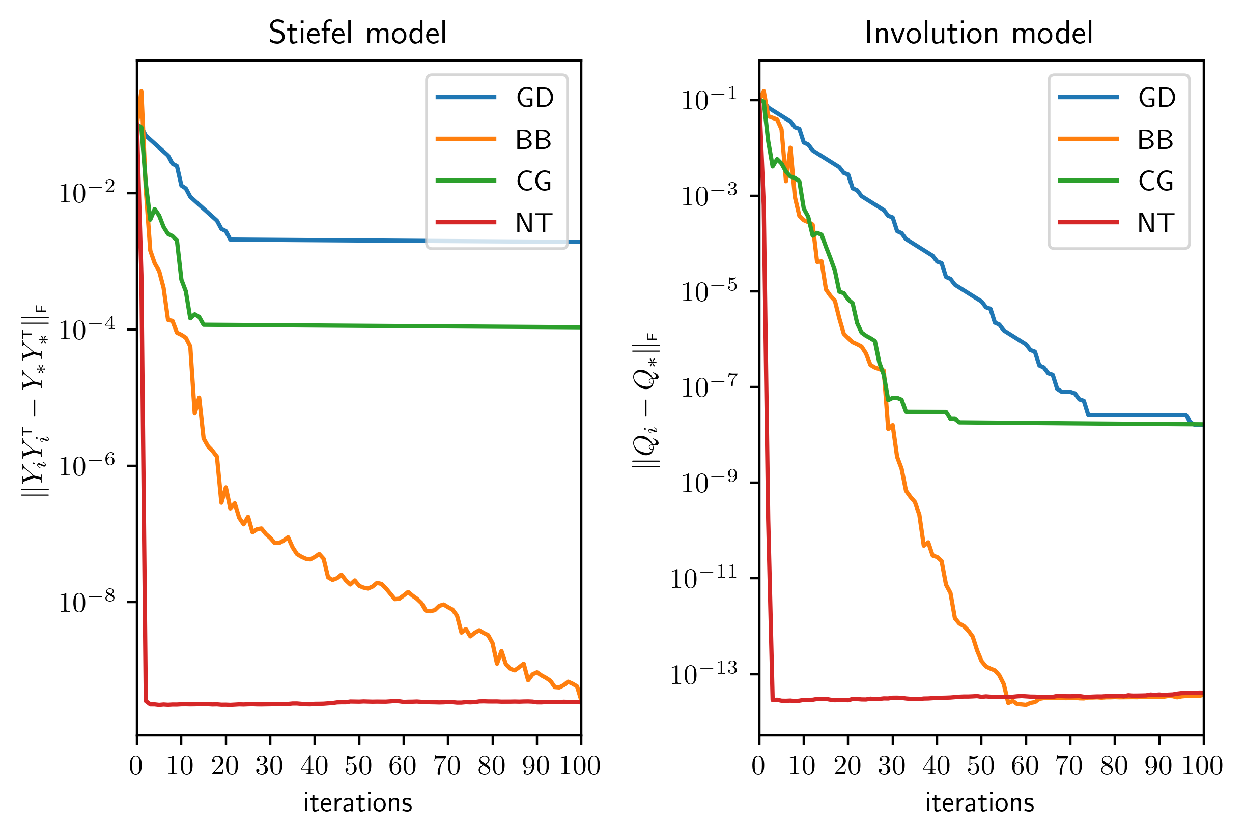
Figure 1. Convergence behavior of algorithms in the Stiefel and involution models.
Refer to caption

Figure 2 shows the loss of orthogonality for various algorithms in the Stiefel and involution models, measured respectively by ‖Yi𝖳​Yi−I‖𝖥\|Y_{i}^{\scriptscriptstyle\mathsf{T}}Y_{i}-I\|_{\scriptscriptstyle\mathsf{F}} and ‖Qi2−I‖𝖥\|Q_{i}^{2}-I\|_{\scriptscriptstyle\mathsf{F}}. In the Stiefel model, the deviation from orthogonality ‖Yi𝖳​Yi−I‖𝖥\|Y_{i}^{\scriptscriptstyle\mathsf{T}}Y_{i}-I\|_{\scriptscriptstyle\mathsf{F}} grows exponentially. In the worst case, the gd iterates YiY_{i}, which of course ought to be of rank k=6k=6, actually converged to a rank-one matrix. In the involution model, the deviation from orthogonality ‖Qi2−I‖𝖥\|Q_{i}^{2}-I\|_{\scriptscriptstyle\mathsf{F}} remains below 10−1310^{-13} for all algorithms — the loss-of-orthogonality is barely noticeable.
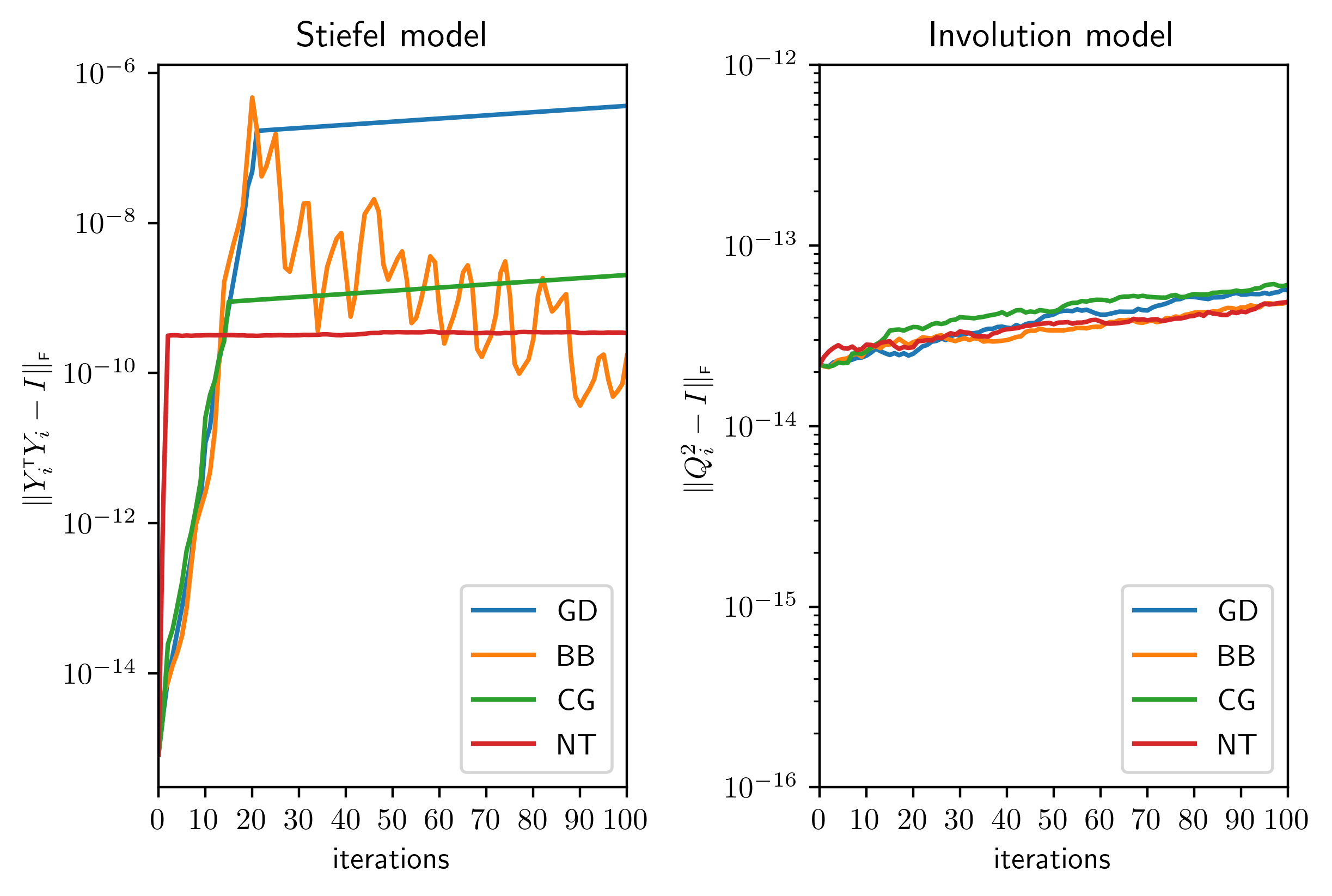
Figure 2. Loss of orthogonality in Stiefel and involution models.
Refer to caption

A closer inspection of the algorithms for nt [23, p. 325] and cg [23, p. 327] in the Stiefel model reveals why: A point YiY_{i} and the gradient GiG_{i} at that point are highly dependent on each other — an ε\varepsilon-deviation from orthogonality in YiY_{i} results in an ε\varepsilon-error in GiG_{i} that in turn becomes a 2​ε2\varepsilon-deviation from orthogonality in Yi+1Y_{i+1}, i.e., one loses orthogonality at an exponential rate. We may of course reorthogonalize YiY_{i} at every iteration in the Stiefel model to artificially enforce the orthonormality of its columns but this incurs additional cost and turns a Riemannian algorithm into a retraction algorithm, as reorthogonalization of YiY_{i} is effectively a qr retraction.

Contrast this with the involution model: In Algorithms 3 (nt) and 4 (cg), the point QiQ_{i} and the effective gradient GiG_{i} are both computed directly from the eigenbasis ViV_{i}, which is updated to Vi+1V_{i+1} by an orthogonal matrix, or a sequence of Givens rotations if one uses Strang splitting as in (47). This introduces a small (constant order) deviation from orthogonality each step. Consequently, the deviation from orthogonality at worst grows linearly.

8.2. Grassmann Procrustes problem

Let k,m,n∈ℕk,m,n\in\mathbb{N} with k≤nk\leq n. Let A∈ℝm×nA\in\mathbb{R}^{m\times n} and B∈ℝm×kB\in\mathbb{R}^{m\times k}. The minimization problem

(54) minQ𝖳​Q=I⁡∥A−B​Q∥𝖥,\min_{Q^{\scriptscriptstyle\mathsf{T}}Q=I}\lVert A-BQ\rVert_{\scriptscriptstyle\mathsf{F}},

is called the Stiefel Procrustes problem [23, Section 3.5.2] and the special case k=nk=n is the usual orthogonal Procrustes problem [30, Section 6.4.1]. Respectively, these are

minQ∈V⁡(k,n)⁡∥A−B​Q∥𝖥andminQ∈O⁡(n)⁡∥A−B​Q∥𝖥.\min_{Q\in\V(k,n)}\lVert A-BQ\rVert_{\scriptscriptstyle\mathsf{F}}\qquad\text{and}\qquad\min_{Q\in\O(n)}\lVert A-BQ\rVert_{\scriptscriptstyle\mathsf{F}}.

One might perhaps wonder if there is also a Grassmann Procrustes problem

(55) minQ∈Gr⁡(k,n)⁡∥A−B​Q∥𝖥.\min_{Q\in\Gr(k,n)}\lVert A-BQ\rVert_{\scriptscriptstyle\mathsf{F}}.

Note that here we require m=nm=n. In fact, with the involution model for Gr⁡(k,n)\Gr(k,n), the problem (55) makes perfect sense. The same argument in the proof of Lemma 6.3 shows that the minimizer Q∗Q_{*} of (55) is given by Q∗=V​Ik,n−k​V𝖳Q_{*}=VI_{k,n-k}V^{\scriptscriptstyle\mathsf{T}} where

A𝖳​B+B𝖳​A2=V​D​V𝖳\frac{A^{\scriptscriptstyle\mathsf{T}}B+B^{\scriptscriptstyle\mathsf{T}}A}{2}=VDV^{\scriptscriptstyle\mathsf{T}}

is an eigendecomposition with eigenbasis V∈O⁡(n)V\in\O(n) and eigenvalues D≔diag⁡(λ1,…,λn)D\coloneqq\diag(\lambda_{1},\dots,\lambda_{n}) in descending order. The convergence and loss-of-orthogonality behaviors for this problem are very similar to those in Section 8.1 and provides further confirmation for the earlier numerical results. The plots from solving (55) for arbitrary A,BA,B using any of Algorithms 2–5 are generated in our codes but given that they are nearly identical to Figures 1 and 2 we omit them here.

8.3. Fréchet mean and Karcher mean

Let Q1,…,Qm∈Gr⁡(k,n)Q_{1},\dots,Q_{m}\in\Gr(k,n) and consider the sum-of-square-distances minimization problem:

(56) min⁡∑j=1mQ∈Gr⁡(k,n)⁡d2​(Qj,Q),\min_{Q\in\Gr(k,n)}\sum_{j=1}^{m}d^{2}(Q_{j},Q),

where dd is the geodesic distance in (29). The global minimizer of this problem is called the Fréchet mean and a local minimizer is called a Karcher mean [41]. For the case m=2m=2, a Fréchet mean is the midpoint, i.e., t=1/2t=1/2, of the geodesic connecting Q1Q_{1} and Q2Q_{2} given by the closed-form expression in Proposition 4.5. The objective function ff in (56) is differentiable almost everywhere55 5 ff is nondifferentiable only when QQ falls on the cut locus of QiQ_{i} for some ii but the union of all cut loci of Q1,…,QmQ_{1},\dots,Q_{m} has codimension ≥1\geq 1. with its Riemannian gradient [40] given by

∇f​(Q)=2​∑j=1mlogQ⁡(Qj),\nabla\!f(Q)=2\sum_{j=1}^{m}\log_{Q}(Q_{j}),

where the logarithmic map is as in Corollary 4.7. To the best of our knowledge, there is no simple expression for ∇2f​(Q)\nabla^{2}\!f(Q) and as such we exclude Newton method from consideration below.
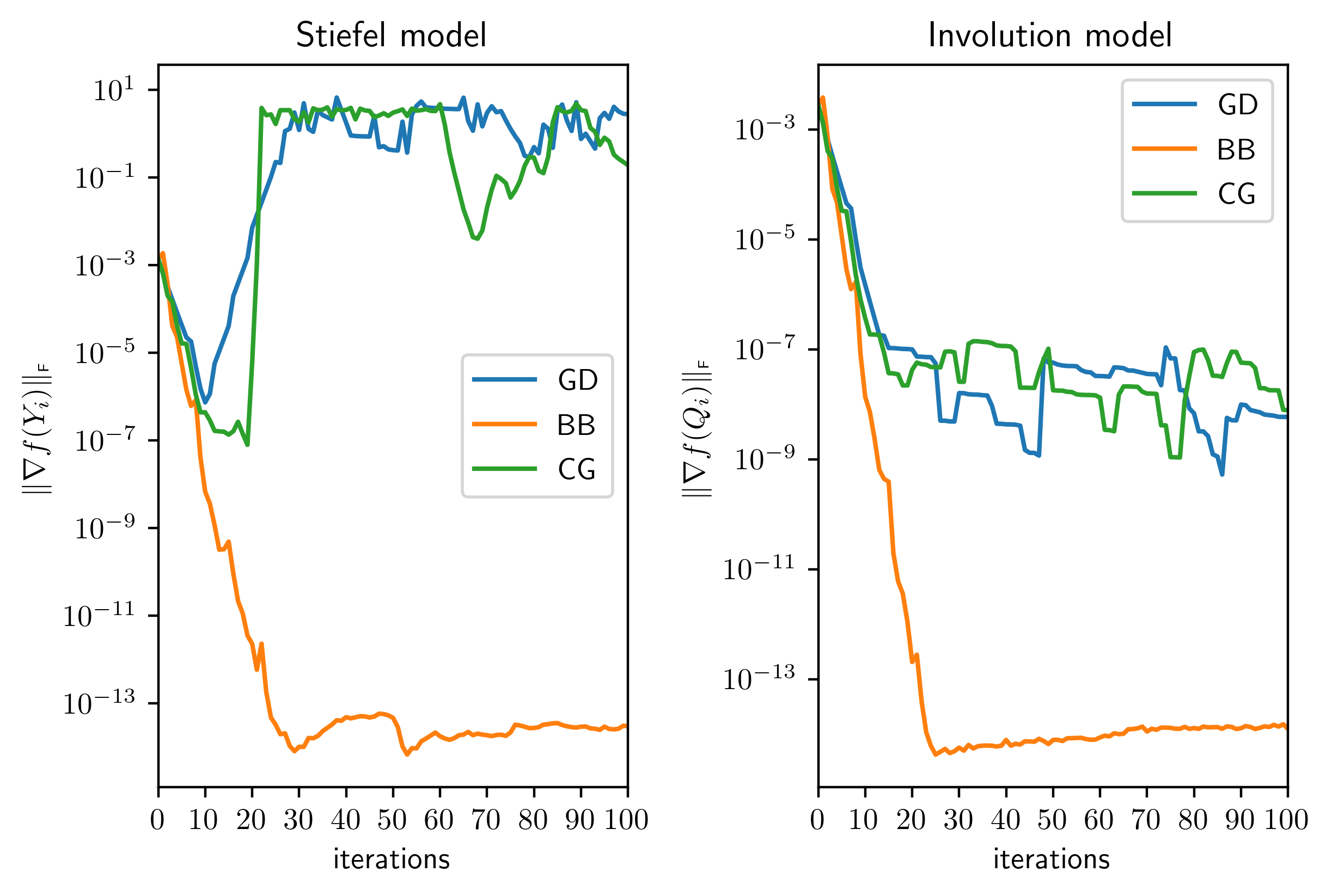
Figure 3. Convergence behavior of algorithms in the Stiefel and involution models.
Refer to caption

We will set k=6k=6, n=16n=16, and m=3m=3. Unlike the problems in Sections 8.1 and 8.2, the problem in (56) does not have a closed-form solution when m>2m>2. Consequently we quantify convergence behavior in Figure 3 by the rate gradient goes to zero. The deviation from orthogonality is quantified as in Section 8.1 and shown in Figure 4. The instability of the algorithms in the Stiefel model is considerably more pronounced here — both gd and cg failed to converge to a stationary point as we see in Figure 3. The cause, as revealed by Figure 4, is a severe loss-of-orthogonality that we will elaborate below.

The expression for geodesic distance d⁡(Y,Y′)d(Y,Y^{\prime}) between two points Y,Y′Y,Y^{\prime} in the Stiefel model (see [2, Section 3.8] or [65, Equation 7]) is predicated on the crucial assumption that each of these matrices has orthonormal columns. As a result, a moderate deviation from orthonormality in an iterate YY leads to vastly inaccurate values in the objective function value f⁡(Y)f(Y), which is a sum of mm geodesic distances squared. This is reflected in the graphs on the left of Figure 3 for the gd and cg algorithms, whose step sizes come from line search and depend on these function values. Using the bb step size, which does not depend on objective function values, avoids the issue. But for gd and cg, the reliance on inaccurate function values leads to further loss-of-orthogonality, and when the columns of an iterate YY are far from orthonormal, plugging YY into the expression for gradient simply yields a nonsensical result, at times even giving an ascent direction in a minimization problem.66 6 This last observation is from a plot of the function values that comes with our code but is not included here.

For all three algorithms in the involution model, the deviation from orthogonality in the iterates is kept at a negligible level of under 10−1310^{-13} over the course of 100 iterations.

Figure 4. Loss of orthogonality in the Stiefel and involution models.
Refer to caption

Acknowledgment

We would like to acknowledge the intellectual debt we owe to [2, 23, 33]. The work in this article would not have been possible without drawing from their prior investigations.

ZL is supported by a Neubauer Family Distinguished Doctoral Fellowship from the University of Chicago. LHL is supported by NSF IIS 1546413, DMS 1854831, and the Eckhardt Faculty Fund. KY is supported by NSFC Grant no. 11688101, NSFC Grant no. 11801548 and National Key R&D Program of China Grant no. 2018YFA0306702.

References

  • [1] H. Abe and T. Matsumura. Schur polynomials and weighted Grassmannians. J. Algebraic Combin., 42(3):875–892, 2015.
  • [2] P.-A. Absil, R. Mahony, and R. Sepulchre. Riemannian geometry of Grassmann manifolds with a view on algorithmic computation. Acta Appl. Math., 80(2):199–220, 2004.
  • [3] P.-A. Absil, R. Mahony, and R. Sepulchre. Optimization algorithms on matrix manifolds. Princeton University Press, Princeton, NJ, 2008.
  • [4] P.-A. Absil and J. Malick. Projection-like retractions on matrix manifolds. SIAM J. Optim., 22(1):135–158, 2012.
  • [5] E. Anderson, Z. Bai, C. Bischof, S. Blackford, J. D. J. Dongarra, J. D. Croz, A. Greenbaum, S. Hammarling, A. McKenney, and D. Sorensen. LAPACK Users’ Guide. SIAM, Philadelphia, PA, third edition, 1999.
  • [6] C. Bachoc, R. Coulangeon, and G. Nebe. Designs in Grassmannian spaces and lattices. J. Algebraic Combin., 16(1):5–19, 2002.
  • [7] A. Barg and D. Y. Nogin. Bounds on packings of spheres in the Grassmann manifold. IEEE Trans. Inform. Theory, 48(9):2450–2454, 2002.
  • [8] J. Barzilai and J. M. Borwein. Two-point step size gradient methods. IMA J. Numer. Anal., 8(1):141–148, 1988.
  • [9] R. Bhatia. Linear algebra to quantum cohomology: the story of Alfred Horn’s inequalities. Amer. Math. Monthly, 108(4):289–318, 2001.
  • [10] A. R. Calderbank, R. H. Hardin, E. M. Rains, P. W. Shor, and N. J. A. Sloane. A group-theoretic framework for the construction of packings in Grassmannian spaces. J. Algebraic Combin., 9(2):129–140, 1999.
  • [11] J. R. Cardoso and F. S. Leite. Exponentials of skew-symmetric matrices and logarithms of orthogonal matrices. J. Comput. Appl. Math., 233(11):2867–2875, 2010.
  • [12] E. Celledoni and A. Iserles. Methods for the approximation of the matrix exponential in a Lie-algebraic setting. IMA J. Numer. Anal., 21(2):463–488, 2001.
  • [13] J. Cheeger and D. G. Ebin. Comparison theorems in Riemannian geometry. AMS Chelsea Publishing, Providence, RI, 2008.
  • [14] Y. Chikuse. Statistics on special manifolds, volume 174 of Lecture Notes in Statistics. Springer-Verlag, New York, NY, 2003.
  • [15] E. S. Coakley, V. Rokhlin, and M. Tygert. A fast randomized algorithm for orthogonal projection. SIAM J. Sci. Comput., 33(2):849–868, 2011.
  • [16] J. H. Conway, R. H. Hardin, and N. J. A. Sloane. Packing lines, planes, etc.: packings in Grassmannian spaces. Experiment. Math., 5(2):139–159, 1996.
  • [17] J. X. da Cruz Neto, L. L. de Lima, and P. R. Oliveira. Geodesic algorithms in Riemannian geometry. Balkan J. Geom. Appl., 3(2):89–100, 1998.
  • [18] Y. H. Dai and Y. Yuan. A nonlinear conjugate gradient method with a strong global convergence property. SIAM J. Optim., 10(1):177–182, 1999.
  • [19] N. Del Buono, L. Lopez, and R. Peluso. Computation of the exponential of large sparse skew-symmetric matrices. SIAM J. Sci. Comput., 27(1):278–293, 2005.
  • [20] J. W. Demmel. Applied numerical linear algebra. SIAM, Philadelphia, PA, 1997.
  • [21] M. P. do Carmo. Riemannian geometry. Mathematics: Theory & Applications. Birkhäuser, Boston, MA, 1992.
  • [22] D. W. Dreisigmeyer. Direct search methods on reductive homogeneous spaces. J. Optim. Theory Appl., 176(3):585–604, 2018.
  • [23] A. Edelman, T. A. Arias, and S. T. Smith. The geometry of algorithms with orthogonality constraints. SIAM J. Matrix Anal. Appl., 20(2):303–353, 1999.
  • [24] M. Ehler and M. Gräf. Reproducing kernels for the irreducible components of polynomial spaces on unions of Grassmannians. Constr. Approx., 49(1):29–58, 2019.
  • [25] M. Farber and A. Postnikov. Arrangements of equal minors in the positive Grassmannian. Adv. Math., 300:788–834, 2016.
  • [26] R. Fletcher and C. M. Reeves. Function minimization by conjugate gradients. Comput. J., 7:149–154, 1964.
  • [27] P. Galashin and P. Pylyavskyy. Ising model and the positive orthogonal Grassmannian. Duke Math. J., 169(10):1877–1942, 2020.
  • [28] E. S. Gawlik, Y. Nakatsukasa, and B. D. Sutton. A backward stable algorithm for computing the CS decomposition via the polar decomposition. SIAM J. Matrix Anal. Appl., 39(3):1448–1469, 2018.
  • [29] D. G. Giovanis and M. D. Shields. Data-driven surrogates for high dimensional models using Gaussian process regression on the Grassmann manifold. Comput. Methods Appl. Mech. Engrg., 370:113269, 2020.
  • [30] G. H. Golub and C. F. Van Loan. Matrix computations. Johns Hopkins Studies in the Mathematical Sciences. Johns Hopkins University Press, Baltimore, MD, fourth edition, 2013.
  • [31] M. Harandi, R. Hartley, C. Shen, B. Lovell, and C. Sanderson. Extrinsic methods for coding and dictionary learning on Grassmann manifolds. Int. J. Comput. Vis., 114(2-3):113–136, 2015.
  • [32] S. Helgason. Differential geometry, Lie groups, and symmetric spaces, volume 34 of Graduate Studies in Mathematics. AMS, Providence, RI, 2001.
  • [33] U. Helmke, K. Hüper, and J. Trumpf. Newton’s method on Graßmann manifolds. https://arxiv.org/abs/0709.2205, 2007.
  • [34] M. R. Hestenes and E. Stiefel. Methods of conjugate gradients for solving linear systems. J. Research Nat. Bur. Standards, 49:409–436 (1953), 1952.
  • [35] N. J. Higham. Accuracy and stability of numerical algorithms. SIAM, Philadelphia, PA, second edition, 2002.
  • [36] N. J. Higham. Functions of matrices. SIAM, Philadelphia, PA, 2008.
  • [37] B. Jiang and Y.-H. Dai. A framework of constraint preserving update schemes for optimization on Stiefel manifold. Math. Program., 153(2, Ser. A):535–575, 2015.
  • [38] J. Jost. Riemannian geometry and geometric analysis. Universitext. Springer, Cham, seventh edition, 2017.
  • [39] V. Jurdjevic, I. Markina, and F. Silva Leite. Extremal curves on Stiefel and Grassmann manifolds. J. Geom. Anal., 108(4):289–318, 2019.
  • [40] H. Karcher. Riemannian center of mass and mollifier smoothing. Comm. Pure Appl. Math., 30(5):509–541, 1977.
  • [41] H. Karcher. Riemannian center of mass and so called Karcher mean. https://arxiv.org/abs/1407.2087, 2014.
  • [42] S. N. Karp. Sign variation, the Grassmannian, and total positivity. J. Combin. Theory Ser. A, 145:308–339, 2017.
  • [43] T. Kato. Perturbation theory for linear operators. Classics in Mathematics. Springer-Verlag, Berlin, 1995.
  • [44] S. Kobayashi and K. Nomizu. Foundations of differential geometry. Vol. II. Wiley Classics Library. John Wiley and Sons, New York, NY, 1996.
  • [45] I. Le and C. Fraser. Tropicalization of positive Grassmannians. Selecta Math. (N.S.), 25(5):Paper No. 75, 55 pp., 2019.
  • [46] P. Mattila. Geometry of sets and measures in Euclidean spaces, volume 44 of Cambridge Studies in Advanced Mathematics. Cambridge University Press, Cambridge, 1995.
  • [47] A. Medra and T. N. Davidson. Incremental Grassmannian feedback schemes for multi-user MIMO systems. IEEE Trans. Signal Process., 63(5):1130–1143, 2015.
  • [48] B. Mishra, H. Kasai, P. Jawanpuria, and A. Saroop. A Riemannian gossip approach to subspace learning on Grassmann manifold. Mach. Learn., 108(10):1783–1803, 2019.
  • [49] B. Mishra and R. Sepulchre. Riemannian preconditioning. SIAM J. Optim., 26(1):635–660, 2016.
  • [50] C. Moler and C. Van Loan. Nineteen dubious ways to compute the exponential of a matrix, twenty-five years later. SIAM Rev., 45(1):3–49, 2003.
  • [51] L. I. Nicolaescu. Lectures on the geometry of manifolds. World Scientific, Hackensack, NJ, second edition, 2007.
  • [52] J. Nocedal and S. J. Wright. Numerical optimization. Springer Series in Operations Research and Financial Engineering. Springer, New York, NY, second edition, 2006.
  • [53] E. Polak and G. Ribière. Note sur la convergence de méthodes de directions conjuguées. Rev. Française Informat. Recherche Opérationnelle, 3(16):35–43, 1969.
  • [54] A. Sarlette and R. Sepulchre. Consensus optimization on manifolds. SIAM J. Control Optim., 48(1):56–76, 2009.
  • [55] G. Sonnevend, J. Stoer, and G. Zhao. On the complexity of following the central path of linear programs by linear extrapolation. II. volume 52, pages 527–553. 1991.
  • [56] G. W. Stewart. Computing the C​SCS decomposition of a partitioned orthonormal matrix. Numer. Math., 40(3):297–306, 1982.
  • [57] G. W. Stewart. Matrix algorithms I: Basic decompositions. SIAM, Philadelphia, PA, 1998.
  • [58] G. Strang. On the construction and comparison of difference schemes. SIAM J. Numer. Anal., 5:506–517, 1968.
  • [59] Y. Sun, N. Flammarion, and M. Fazel. Escaping from saddle points on Riemannian manifolds. In Advances in Neural Information Processing Systems, pages 7276–7286, 2019.
  • [60] L. N. Trefethen and D. Bau, III. Numerical linear algebra. SIAM, Philadelphia, PA, 1997.
  • [61] D. S. Watkins. Fundamentals of matrix computations. Pure and Applied Mathematics. John Wiley and Sons, Hoboken, NJ, third edition, 2010.
  • [62] Z. Wen and W. Yin. A feasible method for optimization with orthogonality constraints. Math. Program., 142(1-2, Ser. A):397–434, 2013.
  • [63] J. H. Wilkinson. The algebraic eigenvalue problem. Monographs on Numerical Analysis. Oxford University Press, New York, NY, 1988.
  • [64] Y.-C. Wong. Differential geometry of Grassmann manifolds. Proc. Nat. Acad. Sci. U.S.A., 57:589–594, 1967.
  • [65] K. Ye and L.-H. Lim. Schubert varieties and distances between subspaces of different dimensions. SIAM J. Matrix Anal. Appl., 37(3):1176–1197, 2016.
  • [66] G. Zhao. Representing the space of linear programs as the Grassmann manifold. Math. Program., 121(2, Ser. A):353–386, 2010.
  • [67] L. Zheng and D. N. C. Tse. Communication on the Grassmann manifold: a geometric approach to the noncoherent multiple-antenna channel. IEEE Trans. Inform. Theory, 48(2):359–383, 2002.
  • [68] W. Ziller. Examples of Riemannian manifolds with non-negative sectional curvature. In Surveys in differential geometry. Vol. XI, volume 11 of Surv. Differ. Geom., pages 63–102. International Press, Somerville, MA, 2007.