Ensemble Forecasting of the Zika Space-Time Spread with Topological Data Analysis
Yulia R. Gel , Department of Mathematical Sciences, University of Texas at Dallas, 800 West Campbell Road, Richardson, TX 75080, USA. E-mail: ygl@utdallas.edu
Ensemble Forecasting of the Zika Space-Time Spread with Topological Data Analysis
Abstract
As per the records of the World Health Organization, the first formally reported incidence of Zika virus occurred in Brazil in May 2015. The disease then rapidly spread to other countries in Americas and East Asia, affecting more than 1,000,000 people. Zika virus is primarily transmitted through bites of infected mosquitoes of the species Aedes (Aedes aegypti and Aedes albopictus). The abundance of mosquitoes and, as a result, the prevalence of Zika virus infections are common in areas which have high precipitation, high temperature, and high population density. Nonlinear spatio-temporal dependency of such data and lack of historical public health records make prediction of the virus spread particularly challenging. In this paper we enhance Zika forecasting by introducing the concepts of topological data analysis and, specifically, persistent homology of atmospheric variables, into the virus spread modeling. The key rationale is that topological summaries allow for capturing higher-order dependencies among atmospheric variables that otherwise might be unassessable via conventional spatio-temporal modelling approaches based on geographical proximity assessed via Euclidean distance. We introduce a new concept of cumulative Betti numbers and then integrate the cumulative Betti numbers as topological descriptors into three predictive machine learning models: random forest, generalized boosted regression, and deep neural network. Furthermore, to better quantify for various sources of uncertainties, we combine the resulting individual model forecasts into an ensemble of the Zika spread predictions using Bayesian model averaging. The proposed methodology is illustrated in application to forecasting of the Zika space-time spread in Brazil in the year 2018.
keywords
Zika virus, epidemics, Bayesian model averaging, machine learning, neural network1 Introduction
The Zika virus is a flavivirus belonging to the Flaviviridae family which also includes yellow fever, dengue, Japanese encephalitis, and West Nile viruses (Goeijenbier et al. 2016). The earliest known occurrence of Zika was identification of the virus in the serum of a rhesus monkey in 1947 in Uganda (Dick et al. 1952; Dick 1952). In 2015 Zika virus was detected in Brazil, with an estimate of 1.3 million infection cases, and rapidly was transmitted to other countries in North and South Americas, as well as East Asia (Heukelbach et al. 2016; Malone et al. 2016). Symptoms of Zika virus infection among humans include headache, fever, reddened eyes, rashes, muscle and joint pain. Furthermore, Zika virus can cause severe birth defects when transmitted from a pregnant woman to her fetus. Given a rapid spread of the infection, the World Health Organization declared Zika an epidemic disease from 2015 to 2016 (WHO 2019).
Zika is primarily transmitted through the bite of infected Aedes aegypti and Aedes albopictus (CDC 2018). As a result, the spreading of Zika virus is significantly accelerated by weather conditions favoring the abundance of the Aedes mosquitoes, for example, in temperate climate zones with high humidity and rainfall (Tjaden et al. 2013; Rees et al. 2018; Muñoz et al. 2017). In addition, the virus can be transmitted from mother to her fetus, also via sexual contacts, blood transfusion, and organ transplantation (WHO 2019).
Modeling and forecasting Zika spread continues to attract an ever increasing attention, and there exist three general methodological directions rooted in mathematics, statistics, and machine learning (Ferraris et al. 2019). Mathematical approaches include vector borne compartmental and mechanistic transmission models (see, e.g., overviews by Manore and Hyman 2016; Caminade et al. 2017; Suparit et al. 2018, and references therein). In turn, statistical methods tend to be largely based on the Box–Jenkins family of models with various exogenous predictors, such as atmospheric variables and data from HealthMap digital surveillance system, Google trends, and Twitter microblogs (see, e.g., McGough et al. 2017; Teng et al. 2017; Castro et al. 2018, and references therein). Finally, machine learning approaches to modeling spread of Zika virus include random forest (RF), boosted regression (BR), and deep feed-forward neural network (DFFN) models (Soliman et al. 2019; Seo et al. 2018). As recently shown by Soliman et al. 2019, the DFFN models tend to deliver more competitive predictive performance than RF and BR. Remarkably, while spatio-temporal epidemiology of (re)emerging infectious diseases has been extensively studied in the environmetrics community before (see, for instance, Nobre et al. 2005; Loh 2011; Self et al. 2018, and references therein) and despite the increasing popularity of DL tools (McDermott and Wikle 2019) in the spatio-temporal environmetrics applications, utility of DL approaches in infectious epidemiology remains largely unexplored.
Furthermore, in this paper we bring the tools of topological data analysis (TDA) to spatio-temporal modeling (Diggle et al. 2005; Torabi 2013; Nobre et al. 2005; Jang et al. 2007; Ugarte et al. 2009), and prediction of the Zika spread. TDA is an emerging methodology at the interface of computational topology, statistics, and machine learning that aims to enhance our understanding on the role of the underlying data shape in dynamics of the data generating process—in our case, the spatio-temporal process of the Zika spread which exhibits a complex nonstationary dependence structure. Since areas with higher quantities of rainfall are principally associated with greater abundance of mosquitoes transmitting Zika (Muñoz et al. 2017), our key idea is to employ TDA to explore the structure and to extract information about the shape of the temperature and precipitation data that may be useful for predicting the spread of Zika infection.
While TDA is found to exhibit high utility in many fields, from genetics to finance to power systems (Gidea and Katz 2018; Saggar et al. 2018; Li et al. 2020), application of TDA within epidemiology (Costa and Škraba 2014; Lo and Park 2018) and even more generally environmetrics (Islambekov and Gel 2019; Islambekov et al. 2019) still remains very limited. In particular, TDA and, specifically, persistent homology have been employed by Costa and Škraba 2014 for analysis of influenza-like illness during the 2008–2013 flu seasons in Portugal and Italy. Most recently, Lo and Park 2018 show explanatory power of TDA for analysis of Zika spread. Particularly, Lo and Park 2018 use persistent homology factors of the Aedes aegypti mosquito occurrence locations as regressors within a linear model and show a high utility of topological features within a spatial cross-validation framework. The findings of Lo and Park 2018 demonstrate that the model with topological features as regressors yields higher coefficient of determination () and lower cross-validation mean squared error than the benchmark linear model without TDA features.
Our method advances the approach of Lo and Park 2018 in multiple ways. In contrast to Lo and Park 2018, who do not consider prediction of Zika incidences over time, our goal is to assess utility of TDA in forecasting future spread of Zika, which is the key towards the outbreak emergency preparedness and response. Since mosquito occurrence locations may vary over time, any Zika prediction model based on topological features of mosquito locations also requires forecasts of the mosquito occurrences. Such forecasts are not readily available and may be highly non-trivial, especially in areas with heterogeneous landscapes as Brazil.
In contrast to Lo and Park 2018, we consider TDA in application to shape analysis of temperature and precipitation rather than mosquito data. Such approach allows us to systematically incorporate the future weather and climate forecasts from national weather services and derived topological features of such forecasts into Zika prediction models. Furthermore, we evaluate predictive utility of TDA based on multiple statistical and machine learning models, such as random forest, generalized boosted regression, and DFFN. We introduce a new topological summary concept cumulative Betti number, which is used as a predictor of future Zika dynamics and found to deliver a more stable performance than conventional topological characteristics.
Finally, to quantify multiple sources of uncertainty, we develop an adaptive ensemble of Zika forecasting models using Bayesian model averaging (BMA). We illustrate our proposed methodology in application to predicting Zika virus spread for all the 26 states of Brazil during the year 2018.
The key contributions of our paper can be summarized as follows:
- •
To the best of our knowledge, this is the first paper introducing topological data features as predictors of future space-time spread of infectious diseases.
- •
To increase stability of the topological summaries and associated derived forecasts, especially under the scenarios with limited sample sizes as in the case of many emerging climate-sensitive infectious diseases, we introduce the notion of cumulative Betti numbers. The proposed cumulative Betti numbers can be used in many other applications, beyond infectious epidemiology, which involve noisy data of moderate sample sizes, e.g., household travel networks and microgrids.
- •
We validate utility of our proposed predictive approach across various nonparametric machine learning models, including deep neural networks, which allows for more systematic and objective assessment of predictive gains (if any) delivered by the proposed topological descriptors.
The remainder of the paper is organized in four major sections: data description, methodology for epidemiological forecasting and validation metrics, results, and discussion. In Section 2, we provide information on the collected Zika rate, population density, and atmospheric data. We introduce our topological data analysis in Section 3.1 and statistical and machine learning forecasting methodology in Section 3.2. Section 3.3 lists the validation metrics, Section 4 is devoted to validation of the proposed modeling approaches to prediction of Zika rate in Brazil. Finally, the paper is concluded with a discussion in Section 5.
2 Data description
Brazil’s Ministry of Health publishes cumulative Zika rate on a weekly basis. However, as with many other vector-borne diseases, the official surveillance records for zika are often incomplete and noisy. For instance, for the year of 2018 the percentage of missing weeks is 28.8%, or 15 weeks out of 52 weeks. In turn, 24 weeks out of 52 weeks are missing in the year of 2017, which is 46.15%. Hence, we analyze monthly records of Zika virus rate per 100,000 individuals, constructed from the cumulative weekly Zika rates published by Brazil’s Ministry of Health (MHB 2018), in each of the 26 states of Brazil and each month during 2017 and 2018.
Considering the strong association between Zika virus transmission and local environmental conditions (Tjaden et al. 2013; Muñoz et al. 2017; Rees et al. 2018, e.g., see), we also collected data for precipitation and air temperature. The weather station data are accessed for all states for years 2017 and 2018 through World-Weather-Online 2018. The forecasted precipitation data for 2018 are obtained from INMET 2019. To ensure consistency in temporal resolutions of zika and atmospheric data, all daily atmospheric variables are aggregated to a monthly scale.
3 Methodology for epidemiological forecasting
3.1 Topological data analysis
Topological data analysis (TDA) is a rapidly emerging methodology at the interface of computational topology, statistics, and machine learning which allows for a systematic multi-lens assessment of the underlying topology and geometry of the data generating process (Zomorodian and Carlsson 2005; Carlsson 2009; Chazal and Michel 2017). In this paper, we primarily employ tools of persistent homology (PH) within the TDA framework. The ultimate idea of PH is to quantify dynamics of topological properties exhibited by the data that live in Euclidean or abstract metric space, at various resolution scales. The PH approach is implemented in the two key steps: first, the underlying hidden topology of the observed data set is approximated using certain combinatorial objects, e.g., simplicial complexes, and then the evolution of these combinatorial objects is studied as the resolution scale varies.
We start with providing a brief overview of the main relevant technical concepts.
Definition 1 (Abstract simplicial complex)
Let be a discrete set. Then, an abstract simplicial complex is a collection of finite nonempty subsets of such that if and , then . If , then is called a -simplex.
In case of an Euclidean space, -simplex corresponds to a convex hull of vertices. Hence, a 0-simplex is a vertex, a 1-simplex is an edge, a 2-simplex is a triangle, and a 3-simplex is a tetrahedron.
One of the most widely used choices for a simplicial complex within the TDA framework is a Vietoris–Rips complex which has gained its popularity due to its computational properties and tractability.
Definition 2 (Vietoris–Rips complex)
Let be a metric space, e.g., and be a set of distinct points of . Let be a scale. Then the Vietoris–Rips complex is an abstract simplicial complex whose finite simplices in have a diameter at most , i.e.,
That is, we form the proximity graph of by joining two points in whenever their pairwise distance is less than . We now consider a sequence of scales and associated nested sequence of VR complexes called a Vietoris–Rips filtration . As a result, we can study evolution of topological summaries, such as number of connected components, loops, etc., that appear and disappear with an increase of scale . Persistent topological features, i.e., those with a longer lifespan over varying resolution tend to be associated with the underling structural organization of the data generating process, while features with a shorter lifespan are likely to be a topological noise.
Figure 1 is an illustration of the Vietoris–Rips filtration process based on a toy example of six points. The filtration starts with a ball of radius 0 () around each point (see Figure 1(a)). As the scale increases to 0.2, 0.5, and 1 (see Figures 1(b), 1(c), and 1(d), respectively), the number of connected components decreases and new topological features, such as the loop, appear.
There exist multiple topological summaries to quantify evolution of topological features over the increasing scale , e.g., barcode, persistent diagrams, persistent landscapes, and Betti numbers (see the discussion in Chazal and Michel 2017, and references therein). In this project we focus on utility analysis of Betti numbers.
Definition 3 (Betti number)
The Betti- number is the rank of the -th homology group. That is, is the number of -dimensional simplicial complex features for a given scale .
For a given scale and a given abstract simplicial complex, e.g., the Vietoris–Rips complex, constructed from the observed point cloud under scale , Betti numbers are simply counts of particular topological features in this abstract simplicial complex. For instance, is the count of connected components in the Vietoris–Rips complex; while and are the numbers of holes and voids in the Vietoris–Rips complex, respectively.
Furthermore, we introduce the concept of cumulative Betti numbers which, as we find, tend to deliver more stable predictive performance for forecasting the Zika spread.
Definition 4 (Cumulative Betti numbers)
Over a sequence of scales , cumulative Betti number , , is defined as the sum of Betti numbers , . That is,
| (1) |
In this paper, due to the limited data records, we use only the numbers as topological descriptors, that is, the cumulative number of connected components. We hypothesize that higher predictive performance delivered by cumulative Betti numbers may be explained by higher robustness of to scale sequence selection under uncertainty due to low sample sizes. We used the function ripsDiag in R package TDA (Fasy et al. 2018) to find the cumulative Betti 0 numbers.
Figure 2 depicts cumulative Betti-0, , numbers based on precipitation amounts and temperature in the states of Acre and Alagoas, Brazil.
To extract the topological characteristics for precipitation () and temperature (), we use the following algorithm.
Let be the number of weather stations in each state and be the corresponding weather observations in month (; , and ). (Here we suppress the superscripts for the sake of notations.) Consider a point cloud for each month and state . We now measure (dis)similarity (in terms of the Euclidean distance) among recorded atmospheric variables in the -th month across all weather stations in the -th state. For instance, in a case of temperature (), we set up (in degrees Celsius) and obtain a distance graph by connecting two weather stations and only if their recorded temperature observation differ at most in degrees Celsius, i.e., . We now count a number of topological features (e.g., a number of connected components, or Betti 0 ) for a given scale . Then we increase scale and repeat the procedure. Summing over consider scales (see (1)) yields a cumulative Betti number for the -th month in the -th state (; ). The idea is that topological summaries allow for capturing higher-order dependencies among atmospheric variables that are unassessable via conventional spatio-temporal modelling approaches based on geographical proximity.
3.2 Models
We employ three statistical and machine learning models to predict the Zika activity at the state level, namely, random forest (RF), boosted regression (BR), and deep feed-forward neural networks (DFFN). Using Bayesian model averaging (BMA), we then develop a multi-model ensemble of the Zika forecasts. We train all the models on the year 2017 data (training set), then evaluate their out-of-sample forecasts using the 2018 data (testing set). Below we provide an overview of the considered modeling approaches and the forecast validation metrics.
Let be the Zika rate in month in state ( and ) and be the corresponding regressors. In each of the models, is the precipitation, is the temperature, is the cumulative Betti-0 for the precipitation, is the cumulative Betti-0 for the temperature, is the categorical variable representing month (January, …, December), is the precipitation lagged by one month, and is the temperature lagged by one month. We added the lagged variables ( and ) to account for delay effects.
Random forest (RF)
The random forest is one of the most popular models in machine learning and statistics, with an idea to combine several individual decision tree models into an additive multi-model ensemble (Breiman 2001):
where is an individual decision or regression tree. The two fundamental ideas behind the RF approach are i) for constructing individual trees , observations from the training set are randomly sampled with replacement (i.e., bootstrapped), and ii) each individual split in a tree is based on a random subset of variables that are used in the model. These concepts of RF allow to reduce the effect of overfitting and to optimize a bias-variance trade-off. We used the function randomForest in R package randomForest (Breiman et al. 2018) to train the random forest model.
Generalized boosted regression model
The model is built on two techniques: decision tree algorithms and boosting methods (Breiman 1997; Friedman 2001; Friedman 2002). Generalized boosted models iteratively fit many decision trees to improve the accuracy of the model.
Let be the number of terminal nodes in a regression tree. The tree partitions the input space into disjoint regions . Each regression tree model itself takes an additive form
where is the value predicted in the region , is the input datum, and is the indicator function. Then, the update at the -th iteration, is
where is a scaling factor and the solution to the “line search”; are the corresponding least-squares coefficients, and are the regions defined by the terminal nodes of the tree at the -th iteration.
Let . Note that a separate choice for optimal value is proposed by Friedman 2001 in each tree region, opposed to a single in an entire tree. Update rule for model now becomes:
| (2) | ||||
| (3) |
where (3) is just the optimal constant update in each terminal node region, based on the loss function , given the current approximation .
Additional boosting algorithm details are available in Ridgeway 2019 and Friedman 2001. For the boosted regression, we used the function gbm in R package gbm (Greenwell et al. 2019) with the number of trees equal to 100 and the interaction depth of 3, chosen through a cross-validation.
Deep feed-forward neural network (DFFN)
The DFFN algorithm (Hagan and Menhaj 1994; Riedmiller and Braun 1993; Zhang et al. 2007) is performed as follows: input data move forward from input to hidden layers to output, and at each of those moves the data are non-linearly transformed (using so-called activation function) and re-weighted. When reaching the output layer, the error is calculated, based on a selected cost function, which reflects how far the DFFN output is with respect to the actual data (i.e., Zika rate) in the training set.
To illustrate the DFFN algorithm, let be the weight connecting the -th neuron in the th layer to the -th neuron in the -th layer, and let be the activation function (we use sigmoid function), where . The activation values at each layer are calculated in the forward procedure as
where is the bias coefficient, analogous to the intercept term in regression models. After calculating the total error at the output layer, a partial derivative of the cost function with respect to each weight and bias term is obtained. We train DFFN using h2o.deeplearning function in R package h2o (LeDell et al. 2019). The optimal structure for DFFN is selected through a cross-validation: with 2 hidden layers, 12 nodes in each layer, and learning rate 0.01.
Bayesian model averaging (BMA)
We evaluate uncertainty of epidemiological forecasts by constructing a weighted multi-model ensemble. This application of BMA enables a combination of multiple models, with their respective weights assigned according to the models’ most recent predictive performance (Hoeting et al. 1999; Raftery et al. 2005; Fragoso et al. 2018).
In this project, we define model weights within a BMA using root mean square error (RMSE) calculated for the training set of data:
where is the observed data point (in our case, the observed Zika rate in -th month of 2017 at the -th state), is the corresponding estimate delivered by the -th model (), is the total size of the training data set, and is the number of models. Then, the resulting weight for the -th model in the BMA ensemble of forecasts is computed as follows:
Now, let () denote an out-of-sample forecast produced by the -th model (in our case, the Zika rate forecast of the -th model for the -th state and -th month in 2018). Then the multi-model BMA forecast for that state is defined as
We set to represent the random forest model, to represent generalized boosted regression, and to correspond to the deep feed-forward neural network.
3.3 Validation metrics
We employ two standard statistical measures of accuracy, that is, root mean square error (RMSE) and mean absolute error (MAE) (Bluman 2009; Peck et al. 2015; Kim and Ahn 2019). Let and be the observed and predicted Zika rates for the -th month in -th state in the testing data set. Then,
where is the size of the testing data set. In addition, correlation between observed and forecasted values is measured through the Pearson correlation coefficient
where denotes average Zika rate across all states of Brazil in year 2018, and is the average of out-of-sample predictions across all the states for the corresponding period.
Lower RMSE, MAE, and higher Pearson correlation coefficient imply better forecasting performance.
4 Results
We train our models based on the data observed in the year of 2017 and use the 2018 data for verification. In particular, let be a vector of Zika rates in the -th month and the -th state of year 2017, and let be a matrix of regressors (i.e., design matrix) in the year of 2017. We now compare the performance of the models with persistent features (i.e., with the full set of inputs ) against the models without persistent features (i.e., including only , , and as the inputs). As Table 1 demonstrates, models with persistent features tend to perform better than models without persistent features.
To address whether predictive power of models with topological features is significantly different from models without topological features, we perform Welch’s -test (Welch 1947; Starnes et al. 2010) on the absolute and squared errors delivered by models with and without topological predictors, under the null hypothesis that topological predictors yield no predictive gain. In addition, we assess whether the deep learning model (i.e., a deep feed-forward network) yields a significantly different predictive gain comparing to random forest and boosted regression.
| With persistent features | Without persistent features | MSE | MAE | |||||
|---|---|---|---|---|---|---|---|---|
| Method | RMSE | MAE | RMSE | MAE | -value | -value | ||
| Random forest | 11.351 | 8.262 | 0.391 | 12.134 | 8.667 | 0.307 | 0.348 | 0.396 |
| Boosted regression | 13.238 | 9.154 | 0.363 | 15.044 | 10.091 | 0.286 | 0.093 | 0.262 |
| DFFN | 8.934 | 6.361 | 0.425 | 10.953 | 8.084 | 0.347 | 0.001 | 0.007 |
| BMA-RMSE | 6.721 | 4.265 | 0.419 | 8.380 | 7.854 | 0.397 | ||
| Model | With persistent features | Without persistent features |
|---|---|---|
| Random forest | 0.002 | 0.277 |
| Boosted regression | 0.203 |
Table 1 indicates that topological features lead to a highly statistically significant predictive gain, while incorporated into the DL DFFN model. However, while topological features result in lower predictive RMSEs for random forest and boosted regression, the predictive gains evaluated using Welch’s -test, appear to be not significant. In turn, Table 2 suggests that DFFN with persistent features delivers the most competitive predictive performance among the three individual models, with Welch’s -test -values of .
As expected, given the DFFN competitiveness, the BMA forecasting results are largely driven by the performance dynamics of DFFN and as such, topological descriptors are found to deliver highly statistically significant forecasting utility within the BMA framework (see Table 1).
For example, the incorporation of the persistent features lowers the RMSE of RF by 6.5%, BR by 12.0%, and DFFN by 18.4%, while the RMSE of the BMA decreases by 19.8%. Similar improvements are observed in terms of MAE, with the MAE of BMA decreasing by 45.7%.
Among the three individual models considered in this study, the tree-based models does not deliver the best forecasting performance. Figure 3(a) shows the RF predictions are grouped above the 45-degree line, denoting over-prediction of the Zika rates; bias of RF is a well known issue (see technical details, e.g., in Chapter 15 by Hastie et al. 2009). The predictions from other models are less biased overall. Particularly, DFFN (Figure 3(c)) and BMA (Figure 3(d)) show a better balance of over-prediction and under-prediction. However, the individual errors are larger (points in the graphs for BR are farther from the 45-degree line) than for RF, see Figure 3(b).
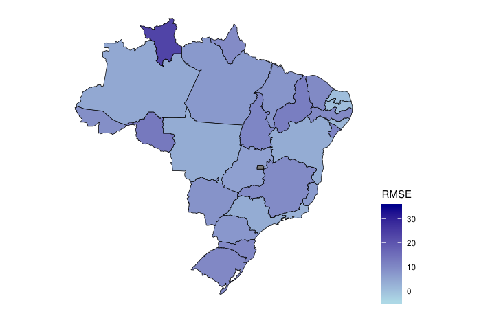


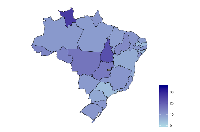
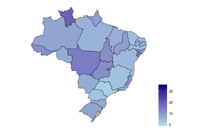
In addition, we examine the geographical distribution of prediction errors of each model. The map in Figure 4 suggests that the BMA-RMSE approach delivers the highest predictive performance for all considered states. Remarkably, among the best predicted states using the BMA-RMSE approach are the states with the highest infection rates, that is, Mato Grosso, Goias, and Mato Grosso do Sul (Ragas 2018, see also Figure 5 showing the average Zika rates, and).



Remark Finally, while Pearson correlations reported in Table 1 are generally low, the resulting correlations appear to be overall on par with the previous studies on zika in other Latin and Southern American countries (McGough et al. 2017). In particular, McGough et al. 2017 report Pearson correlations for 3-week ahead forecast of zika in Honduras not exceeding 0.35 and as low as 0.08. Similar magnitude of Pearson correlations of about 0.30 are found for autoregressive models for 3-week ahead forecast in Colombia, while correlations in El Salvador, Martinique, and Venezuela tend to be somewhat higher. Overall, correlations reported by McGough et al. 2017 tend to vary substantially among countries and among predictive models and to decrease noticeably with the increase of the forecasting horizon.
5 Discussion
Zika continues to be one of the primary healthcare concerns in the Americas, Oceania, Africa and many other parts of the world – making the virus a global challenge for healthcare professional worldwide and demanding the world’s collective preparedness for this climate-sensitive (re)emerging disease.
In this paper we have brought the concepts of topological data analysis of atmospheric variables to enhance prediction of Zika virus. In particular, we have integrated the cumulative Betti numbers as topological descriptors of precipitation and temperature dynamics—one of the key environmental factors in Zika spread—into three predictive machine learning models for Zika: random forest, boosted regression, and deep feed-forward neural network. To better account for various sources of uncertainties and harness the power of individual predictive models, we have combined the resulting individual forecasts into an ensemble of the Zika spread predictions using Bayesian model averaging. Our findings based on the analysis of Zika space-time spread in Brazil have indicated that topological summaries of precipitation dynamics and air temperature contain important predictive information for the future Zika spread.
In the future we plan to advance the proposed topological approach to analysis of other related climate-sensitive diseases such as chikungunya and dengue, not only in Brazil, but also in other countries. Furthermore, epidemiological forecasting can benefit from using the tools of topological data analysis for understanding the spread of diseases through examination of the joint dynamics of topological summaries of the disease rates and associated environmental and socio-economic factors.
Finally, there also exist multiple directions how to better account for various types of uncertainties associated with biosurveillance of emerging climate-sensitive infectious diseases. To address the issue of limited data records and noisy epidemiological information, we plan to integrate various nontraditional data sources, such as webqueries, into surveillance and forecasting of the emerging infectious diseases. Understanding topological summaries of such nontraditional data sources and matching topological patterns of the conventional data from public health units and webqueries can shed a light on future spatial dynamics of the emerging infectious disease. We then plan to employ the semi-parametric bootstrap to develop probabilistic forecasts associated with each model and multiple data sources, which in return can be combined into a joint biosurveillance ensemble.
References
- Bluman (2009) Bluman AG, 2009. Elementary statistics: A step by step approach. McGraw-Hill Higher Education New York.
- Breiman (1997) Breiman L, 1997. Arcing the edge. Technical Report 486. Statistics Department, University of California, Berkeley .
- Breiman (2001) Breiman L, 2001. Random forests. Machine learning 45(1): 5–32.
- Breiman et al. (2018) Breiman L, Cutler A, Liaw A, Wiener M, 2018. randomForest: Breiman and Cutler’s Random Forests for Classification and Regression. R package version 4.6-14.
- Caminade et al. (2017) Caminade C, Turner J, Metelmann S, Hesson JC, Blagrove MSC, Solomon T, Morse AP, Baylis M, 2017. Global risk model for vector-borne transmission of Zika virus reveals the role of El Niño 2015. Proceedings of the National Academy of Sciences 114(1): 119–124.
- Carlsson (2009) Carlsson G, 2009. Topology and data. Bulletin of the American Mathematical Society 46(2): 255–308.
- Castro et al. (2018) Castro MC, Han QC, Carvalho LR, Victora CG, França GV, 2018. Implications of Zika virus and congenital Zika syndrome for the number of live births in Brazil. Proceedings of the National Academy of Sciences 115(24): 6177–6182.
- CDC (2018) CDC, 2018. Centers for disease control and prevention (About Zika).
- Chazal and Michel (2017) Chazal F, Michel B, 2017. An introduction to topological data analysis: Fundamental and practical aspects for data scientists. arXiv Preprint arXiv:1710.04019 .
- Costa and Škraba (2014) Costa JP, Škraba P, 2014. A topological data analysis approach to epidemiology. In European Conference of Complexity Science.
- Dick (1952) Dick G, 1952. Zika virus (II). Pathogenicity and physical properties. Transactions of the Royal Society of Tropical Medicine and Hygiene 46(5): 521–534.
- Dick et al. (1952) Dick G, Kitchen S, Haddow A, 1952. Zika virus (I). Isolations and serological specificity. Transactions of the Royal Society of Tropical Medicine and Hygiene 46(5): 509–520.
- Diggle et al. (2005) Diggle P, Rowlingson B, Su Tl, 2005. Point process methodology for on-line spatio-temporal disease surveillance. Environmetrics: The official journal of the International Environmetrics Society 16(5): 423–434.
- Fasy et al. (2018) Fasy BT, Kim J, Lecci F, Maria C, Millman DL, Rouvreau V, Morozov D, Bauer U, Kerber M, Reininghaus J, 2018. TDA: Statistical Tools for Topological Data Analysis. R package version 1.6.4.
- Ferraris et al. (2019) Ferraris P, Yssel H, Missé D, 2019. Zika virus infection: An update. Microbes and infection .
- Fragoso et al. (2018) Fragoso TM, Bertoli W, Louzada F, 2018. Bayesian model averaging: A systematic review and conceptual classification. International Statistical Review 86(1): 1–28.
- Friedman (2001) Friedman JH, 2001. Greedy function approximation: a gradient boosting machine. Annals of Statistics 29(5): 1189–1232.
- Friedman (2002) Friedman JH, 2002. Stochastic gradient boosting. Computational Statistics & Data Analysis 38(4): 367–378.
- Gidea and Katz (2018) Gidea M, Katz Y, 2018. Topological data analysis of financial time series: Landscapes of crashes. Physica A: Statistical Mechanics and Its Applications 491: 820–834.
- Goeijenbier et al. (2016) Goeijenbier M, Slobbe L, Van der Eijk A, de Mendonça Melo M, Koopmans M, Reusken C, 2016. Zika virus and the current outbreak: an overview. Neth J Med 74(3): 104–9.
- Greenwell et al. (2019) Greenwell B, Boehmke B, Cunningham J, Developers G, 2019. gbm: Generalized Boosted Regression Models. R package version 2.1.5.
- Hagan and Menhaj (1994) Hagan MT, Menhaj MB, 1994. Training feedforward networks with the Marquardt algorithm. IEEE Transactions on Neural Networks 5(6): 989–993.
- Hastie et al. (2009) Hastie TJ, Tibshirani RJ, Friedman JH, 2009. The Elements of Statistical Learning: Data Mining, Inference, and Prediction. Springer, New York, 2 edition.
- Heukelbach et al. (2016) Heukelbach J, Alencar CH, Kelvin AA, de Oliveira WK, de Góes Cavalcanti LP, 2016. Zika virus outbreak in Brazil. The Journal of Infection in Developing Countries 10(02): 116–120.
- Hoeting et al. (1999) Hoeting JA, Madigan D, Raftery AE, Volinsky CT, 1999. Bayesian model averaging: a tutorial. Statistical Science 14(4): 382–401.
- INMET (2019) INMET, 2019. Instituto nacional de meteorologia. http://www.inmet.gov.br/portal/index.php?r=home2/index.
- Islambekov and Gel (2019) Islambekov U, Gel YR, 2019. Unsupervised space–time clustering using persistent homology. Environmetrics 30(4): e2539.
- Islambekov et al. (2019) Islambekov U, Yuvaraj M, Gel YR, 2019. Harnessing the power of topological data analysis to detect change points. Environmetrics : e2612.
- Jang et al. (2007) Jang MJ, Lee Y, Lawson AB, Browne WJ, 2007. A comparison of the hierarchical likelihood and bayesian approaches to spatial epidemiological modelling. Environmetrics: The official journal of the International Environmetrics Society 18(7): 809–821.
- Kim and Ahn (2019) Kim J, Ahn I, 2019. Weekly ILI patient ratio change prediction using news articles with support vector machine. BMC Bioinformatics 20(1): 259.
- LeDell et al. (2019) LeDell E, Gill N, Aiello S, Fu A, Candel A, Click C, Kraljevic T, Nykodym T, Aboyoun P, Kurka M, Malohlava M, 2019. h2o: R Interface for ‘H2O’. R package version 3.26.0.2.
- Li et al. (2020) Li B, Ofori-Boateng D, Gel YR, Zhang J, 2020. A hybrid approach for transmission grid resilience assessment using reliability metrics and power system local network topology. Sustainable and Resilient Infrastructure : 1–16.
- Lo and Park (2018) Lo D, Park B, 2018. Modeling the spread of the Zika virus using topological data analysis. PloS One 13(2): e0192120.
- Loh (2011) Loh JM, 2011. K-scan for anomaly detection in disease surveillance. Environmetrics 22(2): 179–191.
- Malone et al. (2016) Malone RW, Homan J, Callahan MV, Glasspool-Malone J, Damodaran L, Schneider ADB, Zimler R, Talton J, Cobb RR, Ruzic I, et al., 2016. Zika virus: medical countermeasure development challenges. PLoS Neglected Tropical Diseases 10(3): e0004530.
- Manore and Hyman (2016) Manore C, Hyman M, 2016. Mathematical models for fighting Zika virus. Siam News .
- McDermott and Wikle (2019) McDermott PL, Wikle CK, 2019. Deep echo state networks with uncertainty quantification for spatio-temporal forecasting. Environmetrics 30(3): e2553.
- McGough et al. (2017) McGough SF, Brownstein JS, Hawkins JB, Santillana M, 2017. Forecasting Zika incidence in the 2016 Latin America outbreak combining traditional disease surveillance with search, social media, and news report data. PLoS Neglected Tropical Diseases 11(1): e0005295.
- MHB (2018) MHB, 2018. Ministry of Health of Brazil. http://portalms.saude.gov.br/boletins-epidemiologicos.
- Muñoz et al. (2017) Muñoz ÁG, Thomson MC, Stewart-Ibarra AM, Vecchi GA, Chourio X, Nájera P, Moran Z, Yang X, 2017. Could the recent Zika epidemic have been predicted? Frontiers in Microbiology 8: 1291.
- Nobre et al. (2005) Nobre AA, Schmidt AM, Lopes HF, 2005. Spatio-temporal models for mapping the incidence of malaria in pará. Environmetrics 16(3): 291–304.
- Peck et al. (2015) Peck R, Olsen C, Devore JL, 2015. Introduction to statistics and data analysis. Cengage Learning.
- Raftery et al. (2005) Raftery AE, Gneiting T, Balabdaoui F, Polakowski M, 2005. Using Bayesian model averaging to calibrate forecast ensembles. Monthly Weather Review 133(5): 1155–1174.
- Ragas (2018) Ragas J, 2018. Revisiting global health from the periphery: the Zika virus. História, Ciências, Saúde-Manguinhos 25(4): 1185–1187.
- Rees et al. (2018) Rees EE, Petukhova T, Mascarenhas M, Pelcat Y, Ogden NH, 2018. Environmental and social determinants of population vulnerability to Zika virus emergence at the local scale. Parasites & Vectors 11(1): 290.
- Ridgeway (2019) Ridgeway G, 2019. Generalized boosted models: A guide to the gbm package. Update 1(1): 2019.
- Riedmiller and Braun (1993) Riedmiller M, Braun H, 1993. A direct adaptive method for faster backpropagation learning: The RPROP algorithm. In Proceedings of the IEEE International Conference on Neural Networks, volume 1993, San Francisco, CA, 586–591.
- Saggar et al. (2018) Saggar M, Sporns O, Gonzalez-Castillo J, Bandettini PA, Carlsson G, Glover G, Reiss AL, 2018. Towards a new approach to reveal dynamical organization of the brain using topological data analysis. Nature Communications 9(1): 1399.
- Self et al. (2018) Self SCW, McMahan CS, Brown DA, Lund RB, Gettings JR, Yabsley MJ, 2018. A large-scale spatio-temporal binomial regression model for estimating seroprevalence trends. Environmetrics 29(8): e2538.
- Seo et al. (2018) Seo J, Lee J, Kim K, 2018. Decoding of polar code by using deep feed-forward neural networks. In 2018 International Conference on Computing, Networking and Communications (ICNC), IEEE, 238–242.
- Soliman et al. (2019) Soliman M, Lyubchich V, Gel YR, 2019. Complementing the power of deep learning with statistical model fusion: Probabilistic forecasting of influenza in Dallas County, Texas, USA. Epidemics 28: 100345.
- Starnes et al. (2010) Starnes DS, Yates D, Moore DS, 2010. The practice of statistics. Macmillan.
- Suparit et al. (2018) Suparit P, Wiratsudakul A, Modchang C, 2018. A mathematical model for Zika virus transmission dynamics with a time-dependent mosquito biting rate. Theoretical Biology and Medical Modelling 15(1): 11.
- Teng et al. (2017) Teng Y, Bi D, Xie G, Jin Y, Huang Y, Lin B, An X, Feng D, Tong Y, 2017. Dynamic forecasting of Zika epidemics using Google Trends. PloS One 12(1): e0165085.
- Tjaden et al. (2013) Tjaden NB, Thomas SM, Fischer D, Beierkuhnlein C, 2013. Extrinsic incubation period of dengue: Knowledge, backlog, and applications of temperature dependence. PLoS Neglected Tropical Diseases 7(6): e2207.
- Torabi (2013) Torabi M, 2013. Spatio–temporal modeling for disease mapping using car and b-spline smoothing. Environmetrics 24(3): 180–188.
- Ugarte et al. (2009) Ugarte M, Goicoa T, Ibanez B, Militino A, 2009. Evaluating the performance of spatio-temporal bayesian models in disease mapping. Environmetrics: The official journal of the International Environmetrics Society 20(6): 647–665.
- Welch (1947) Welch BL, 1947. The generalization of student’s’ problem when several different population variances are involved. Biometrika 34(1/2): 28–35.
- WHO (2019) WHO, 2019. World Health Organization. http://www.who.int/emergencies/diseases/zika/en/.
- World-Weather-Online (2018) World-Weather-Online, 2018. www.worldweatheronline.com/.
- Zhang et al. (2007) Zhang JR, Zhang J, Lok TM, Lyu MR, 2007. A hybrid particle swarm optimization–back-propagation algorithm for feedforward neural network training. Applied Mathematics and Computation 185(2): 1026–1037.
- Zomorodian and Carlsson (2005) Zomorodian A, Carlsson G, 2005. Computing persistent homology. Discrete & Computational Geometry 33(2): 249–274.