ATLAS Violating CP EffectivelyPreprint: IPPP/20/43
Abstract
CP violation beyond the Standard Model (SM) is a crucial missing piece for explaining the observed matter-antimatter asymmetry in the Universe. Recently, the ATLAS experiment at the Large Hadron Collider has performed an analysis of electroweak production, thereby excluding the SM locally at 95% confidence level in the measurement of CP-sensitive observables. We take the excess’ interpretation in terms of anomalous gauge-Higgs interactions at face value and discuss further steps that are required to scrutinize its origin. In particular, we discuss the relevance of multi-boson production using adapted angular observables to show how they can be used to directly tension the reported excess in a more comprehensive analysis. To connect the excess to a concrete UV scenario for which the underlying assumptions of the analysis are valid, we identify vector-like leptons as a candidate theory consistent with the observed CP-odd Wilson coefficient hierarchy observed by ATLAS. We perform a complete one-loop matching calculation to motivate further model-specific and correlated new physics searches. In parallel, we provide estimates of the sensitivity reach of the LHC’s high luminosity phase for this particular scenario of CP-violation in light of electroweak precision and Run-2 Higgs data. These provide strong constraints on the model’s CP-even low-energy phenomenology, but also inform the size of the CP-odd SM deformation indirectly via our model hypothesis.
I Introduction
The search for non-Standard Model (SM) sources of CP violation is a crucial missing piece in connecting the phenomenological success of the SM so far with its apparent shortcomings related to the observed baryon anti-baryon asymmetry Sakharov 1967. Searches for CP violation in various channels at the Large Hadron Collider (LHC) are therefore a key part of the ongoing experimental program (see e.g. Aad et al. 2020a; Sirunyan et al. 2020a for recent analyses in the context of Higgs physics).
In particular, ATLAS has recently performed a detailed analysis of electroweak production in Ref. Aad et al. 2020b, where it also interprets measurements in terms of effective field theory (EFT) deformations of the SM using dimension six CP-violating operators in the Warsaw basis, Grzadkowski et al. 2010
| (1) | ||||
| (2) |
where denote the field strengths of weak and hypercharge , is the Higgs doublet, are the Pauli matrices, and the tilde refers to the dual field strength tensor (). Using the effective Lagrangian
| (3) |
ATLAS provides the observed 95% confidence level constraints on the following CP violating operators Aad et al. 2020b
| (4) |
based on dimension six interference-only contributions arising from matrix elements
| (5) |
This leads to asymmetries in -sensitive distributions, such as the “signed” (according to rapidity) azimuthal angle difference of the tagged jets . The benefit of such observables and the study of their asymmetries is that the CP-even deformations do not contribute to the exclusion constraints directly, which also extends to CP-even modifications arising from “squared” dimension six contributions. In Eq. (5), denotes the amplitude contribution from the operators of Eq. (1), thus it is a linear function of (as we are keeping terms up to order ).
The constraint on the Wilson coefficient in Eq. (4) indicates a tension with the SM while the observed cross section agrees well with the SM expectation with fb data Arnold et al. 2009; Baglio et al. 2014; Bellm et al. 2016. This prompts us to the following interesting questions.
Firstly, the tension of Eq. (4) seems to rule out the SM at an SM-compatible cross sections. Experimental analyses of asymmetries are challenging, and systematics are crucial limiting factors of distribution shape analyses. Nonetheless, the result of Ref. Aad et al. 2020b could indeed be the first glimpse of a phenomenologically required and motivated extension of the SM, thus deserving further experimental and theoretical scrutiny.
Secondly, limiting ourselves to a subset of the dimension six operators that could in principle contribute to physical process can be theoretically problematic, in particular when we wish to interpret the experimental findings in a truly model-independent fashion. While concrete UV scenarios can be expected to exhibit hierarchical Wilson coefficient patterns, it is not a priori clear that limiting oneself to anomalous gauge boson interactions has a broad applicability to UV scenarios.
Addressing these two questions from a theoretical and phenomenological perspective is the purpose of this work. In Sec. II, we motivate additional diboson analyses of the current data set that will allow us to tension or support the results of Eq. (4) straightforwardly. This is particularly relevant as the ATLAS constraints amount to a large, and as it turns out non-perturbative, amount of CP violation associated with a single direction in the EFT parameter space. In Sec. III, we show that the ATLAS assumptions of considering two operators are consistent for models of vector-like leptons, which can not only reproduces a hierarchy as suggested by Ref. Aad et al. 2020b, but also collapse the analysis-relevant operators to those modifying the gauge boson self-interactions for the considered analyses. Combining both aspects, in Sec. IV we assess the future of diboson and analyses from a perturbative perspective and discuss the high-luminosity (HL) sensitivity potential of the LHC in light of the electroweak precision constraints. We conclude in Sec. V.
II Scrutinizing with diboson production and current LHC data
Deviations related to the gauge boson self-coupling structure can be scrutinized using abundant diboson production at the LHC. With clear leptonic final states and large production cross sections, these signatures are prime candidates for electroweak precision analyses in the LHC environment with only a minimum of background pollution, see also Aad et al. 2011; Chatrchyan et al. 2014. In particular, radiation zeros observed in production are extremely sensitive to perturbations of the SM CP-even coupling structures Goebel et al. 1981; Brodsky and Brown 1982; Brown et al. 1983; Baur et al. 1993; Baur et al. 1994; Han 1995; Aihara et al. 1995. In this section, we discuss the relevant processes that can be employed to further tension the findings of Eq. (4).
II.1 Processes
The squared amplitude of Eq. (5) receives interference contributions from dimension six operators that in the special case where they are CP-odd, do not change the cross section of a process but appear in CP-sensitive observables. Anomalous weak boson interactions were studied in Ref. Aad et al. 2020b through the channel by the introduction of two CP-violating operators, and , modifying the differential distribution of the parity-sensitive signed azimuthal angle between the two final state jets , where () is the azimuthal angle of the first (second) jet, as ordered by rapidity. Similar parity-sensitive observables can be constructed for the leptonic final states of the , , and channels allowing to further constrain the reach of the two Wilson coefficients.
The operators are modeled using FeynRules Christensen and Duhr 2009; Alloul et al. 2014 and exporting the interactions through a UFO Degrande et al. 2012 file. Events are generated using MadEvent Alwall et al. 2011; de Aquino et al. 2012; Alwall et al. 2014 through the MadGraph framework Alwall et al. 2014 and saved in the LHEF format Alwall et al. 2007, before imposing selection criteria and cuts.
production at the LHC
We study the channel by selecting leptons in the pseudorapidity and transverse momentum GeV regions. Exactly three leptons are required and at least one same-flavor opposite-charge lepton pair must have an invariant mass within the boson mass window GeV. In the case of more than one candidate pairs, the one that yields an invariant mass closest to the boson is selected. The remaining lepton is required to have GeV. To obtain a P-sensitive observable, we reconstruct the dilepton pair four-momentum and obtain the rapidity and azimuthal angle . We order the dilepton and third lepton azimuthal angles based on the rapidities of the two reconstructed objects, such that () is the one with the greatest (smallest) rapidity. The signed azimuthal angle is then constructed as .
The distributions of the signed azimuthal angle for both the SM and the SM-BSM interference are normalized to the CMS measured fiducial cross section Khachatryan et al. 2017 of the particular phase space region at TeV center of mass energy
| (6) |
production at the LHC
Turning to the channel and following Ref. Aaboud et al. 2019, we produce events decaying to the final state. The two leptons and are required to satisfy and GeV with no third lepton in the GeV region. Contributions from the Drell-Yan background are reduced by imposing cuts on the missing energy GeV and on the transverse momentum of the dilepton pair GeV. The phase space region is constrained further by enforcing the invariant mass condition GeV that suppresses the background. In this channel the signed azimuthal angle is then defined directly from the azimuthal angles of the two leptons sorted by rapidity.
The fiducial cross section of was measured by ATLAS Aaboud et al. 2019 as
| (7) |
which is used to normalize the calculated differential distribution of . The total cross section of the events as well as the relative statistical and systematic uncertainties are subsequently rescaled to include the final states of all light leptons .
production at the LHC
To obtain the cross section of at TeV, we first use MCFM Campbell and Ellis 1999; Campbell et al. 2011; Campbell et al. 2015; Boughezal et al. 2017; Campbell and Neumann 2019 with generation level cuts GeV and for both leptons and photons, requiring the separation , in order to obtain the cross section at NLO precision with as the renormalization and factorization scale. We have validated these choices against early measurements from ATLAS Aad et al. 2011 and CMS Chatrchyan et al. 2014. The events are generated as before with MadEvent using the same generation cuts and we rescale the computed MadEvent cross section of the events to the MCFM value, in order to include higher order effects and obtain normalized distributions.
Post-generation we veto events without at least one lepton (photon) with transverse momentum GeV ( GeV and require a separation of . The azimuthal angles of the photon and the lepton are sorted by rapidity and is calculated similarly to the other channels.
We assume that the relative statistical and systematic errors that can be calculated from the measured cross section of Ref. Chatrchyan et al. 2014 ** * for this cross section indicates each type of light lepton (, ) and not a sum over them.
| (8) |
will remain the same for the case of TeV and use this in the following statistical analysis.
II.2 Analysis of CP-sensitive observables
To study the allowed region of the parameter space based on current experimental data at the LHC, we consider the differential distribution
| (9) |
where, depending on the process, , and and are constructed from and , respectively, and derive from MC integration of Eq. (5). We generate events for each process using the two coupling reference points and and can rescale distributions using the linear relation of Eq. (5) to subsequently scan over the space of the two CP-odd Wilson coefficients, performing a fit, in order to obtain limits. The statistics is defined as
| (10) |
where is the number of events at a particular luminosity based on the bin of the differential distribution Eq. (9) for a set of Wilson coefficients and is the bin’s expected number of events based solely on the SM. The covariance matrix includes the relative statistical and systematic uncertainties†† † Luminosity uncertainties are treated as systematics. from the experimental measurements, obtained from the aforementioned fiducial cross sections Eqs. (6), (7), and (8) for each process and included in as terms of the form , assuming that both relative and systematic errors are fully correlated. and denote the relative statistical and systematic uncertainties of each process.
We define the confidence intervals with
| (11) |
using the distribution of degrees of freedom , where is obtained by subtracting the number of Wilson coefficients from the number of measurements.
We perform a scan based on an integrated luminosity of fb to obtain the confidence level contours shown in Fig. 1. The results are overlapped with the allowed region from ATLAS Aad et al. 2020b, as well as the best fit point from experimental data, while the does not constrain the region enough to appear on the plot. To obtain the contours, we have tuned a covariance matrix on the basis of the information of Ref. Aad et al. 2020b to obtain the exclusions reported in their work.
As can be seen the measurement of is considerably more sensitive to than to , which results from a combination of accessing -channel momentum transfers in the weak boson fusion-type selections and the boson having a larger overlap with the field than the photon. The latter is also the reason why production enhances the sensitivity in the direction. We note that electroweak mono-photon production in association with two jets is more challenging due to jet-misidentification, and thus does not provide significant sensitivity compared to prompt production.
II.3 HL-LHC extrapolation
We repeat the analysis with the same technique but using an integrated luminosity of ab to obtain contours for HL-LHC. Systematic errors could be significantly reduced at HL-LHC, however for this particular case we find that the fact that BSM contributions are antisymmetric functions, in contrast to the symmetric SM differential distribution, leads to cancellations of the introduced errors in the .‡‡ ‡ The same occurs if the absolute systematic errors are distributed according to a symmetric shape distribution across the bins, instead of using relative errors. Hence, the analysis is predominantly limited only by the statistical fluctuations. The extrapolated contours for ab are shown in Fig. 2.
III Vector-like leptons as a model for -targeted (di-)boson signals
Let us return to the examining the excess related to from a UV model perspective. To this end, we extend the SM by three heavy vector-like lepton (VLL) multiplets Angelescu and Huang 2020
| (12) |
where the quantum numbers are depicted in convention.
The most-general gauge-invariant renormalizable Lagrangian involving these heavy VLLs can be written as
| (13) |
where, , and are the masses of , and , respectively. are the left (right) chiral projection operator. ’s are the complex Yukawa couplings. We will consider , i.e., all the VLLs are degenerate in this work.§§ § This model is also discussed in some detail in Refs. Corbett et al. 2018; Das Bakshi et al. 2019; Angelescu and Huang 2020. We will see that this class of models provides the appropriate UV backdrop of for the Wilson coefficient analysis that we have performed above, and on which Ref. Aad et al. 2020b relies.
III.1 Wilson Coefficients
We integrate out all three heavy degenerate VLL multiplets, see Eq. (13) leading to the effective Lagrangian
| (14) |
where , denote the effective dimension six operators and the Wilson coefficients respectively. The UV theory in Eq. (13) is suitably matched to the SMEFT at the scale which serves as the cut-off scale of the EFT. Here, the factor signifies that all the effective operators are generated through one-loop. And we separate off the loop factor from the definition of the Wilson coefficients , i.e. and in comparison with Eq. (3). We employ the renormalization scheme and also set the RG scale at . Integrating out heavy fermions from UV theories is discussed in Refs. Angelescu and Huang 2020; Ellis et al. 2020. Note that dimension eight CP-violating effects play a subdominant role when perturbative matching is possible in the first place, see Bélusca-Maïto et al. 2018; Corbett et al. 2018. We can therefore expect the dimension six deformations to play a dominant role.
We present the effective operators in the Warsaw basis Grzadkowski et al. 2010 and their respective Wilson coefficients (WCs) are encapsulated in Tab. 1. We also provide the matching using strongly-interacting Light Higgs (SILH)-like convention of Angelescu and Huang 2020 (see also Giudice et al. 2007; Contino et al. 2013) in Tab. 5 of Appendix A for convenience. We compute the most generic results using the complete Lagrangian including CP conserving and violating interactions simultaneously. A subset of our generic results (in SILH-like basis) is in well agreement with operators computed in Ref. Angelescu and Huang 2020. The results in WARSAW for this VLL scenario has been computed for the first time in this paper.¶¶ ¶ In Ref. Angelescu and Huang 2020 the contributions from CP violating (CPV) couplings into the CP-even operators are not considered. We find 19 effective operators with non-zero Wilson coefficients (16 CP-even + 3 CP-odd). In the renormalizable Lagrangian, the VLLs interact with the SM Higgs doublet and that explains the origin of 10 bosonic along with 9 fermionic effective operators accompanied by non-zero WCs. These appear due to application of the equation of motion of the SM Higgs doublet on the effective Lagrangian.
| Operators | Operator Structures | |
Here, we define the following functions to express the WCs in much more compact form Angelescu and Huang 2020 in Tab. 1
| (15) | |||
| (16) |
where, . We further use the additional abbreviations for the same purpose Angelescu and Huang 2020
| (17) |
Here, we denote the electron ()-, up ()-, and down ()-types Standard Model Yukawa couplings as respectively while we refer to the SM Higgs quartic self-coupling as .
The operators that may affect the couplings of gauge bosons to fermion currents, i.e., the relevant LHC processes are Grzadkowski et al. 2010; Brivio et al. 2017; Dedes et al. 2017
| (18) | |||
| (19) |
We have a relevant CP-even operator that leads to an additional contribution to oblique corrections Golden and Randall 1991; Holdom and Terning 1990; Altarelli and Barbieri 1991; Peskin and Takeuchi 1990; Grinstein and Wise 1991; Altarelli et al. 1992; Peskin and Takeuchi 1992; Burgess et al. 1994 and in particular the parameter. In later section, we discuss the impact of all relevant CP-even operators in Electro Weak Precision Observables (EWPOs) in detail. At this point it is worthy to mention that the operators
| (20) | |||
| (21) |
do not modify trilinear gauge interactions as their contributions either vanish due to momentum conservation or can be absorbed into field and coupling redefinitions respecting gauge invariance. By investigating Tab. 1, we also find that our adopted scenario, Eq. (13), predicts . Thus, together with our previous observations, we conclude that is the only relevant operator to interpret the results of ATLAS within the vector-like lepton framework.
In passing we would like to mention that some of the remaining non-zero operators can be probed in Higgs-boson associated final states or (to a lesser extent) through their radiative correction contributions Grojean et al. 2013; Englert and Spannowsky 2015 (the latter corresponds to a two-loop suppression in the considered vector-like lepton UV completion). These processes provide additional CP sensitivity, however, at smaller Higgs-boson related production cross sections (see e.g. the discussion in Ref. Bernlochner et al. 2019) that receive corrections from a range of non-zero Wilson coefficients . We will not investigate Higgs-CP related effects in this work as neither they contribute to the electroweak precision observables nor impact the discussion of the previous section.∥∥ ∥ The additional chiral symmetry violation that leads to non-vanishing Wilson coefficients could in principle be traced into a uniform modification of the Higgs 2-point function Englert et al. 2019 that can in principle be probed at hadron colliders. A related investigation was performed recently by CMS in four top final states Sirunyan et al. 2020b. Sensitivity, however, is currently too limited for this effect to play an important role in a global fit.
| Effective operators | Constrained | Constrained |
|---|---|---|
| (Warsaw) | by EWPO | by Higgs-data |
| ✓ | ✓ | |
| ✓ | ✓ | |
| ✓ | ✓ | |
| ✗ | ✓ | |
| ✗ | ✓ | |
| ✓ | ✓ | |
| ✗ | ✓ | |
| ✗ | ✓ | |
| ✗ | ✓ |
III.2 Constraints from Electroweak Precision Observables and Higgs-data
| VLLs: | Fitted values of parameters |
|---|---|
| Yukawa couplings | (@ 68% C.L.) |
The CP-even SMEFT operators contribute to the Electroweak Precision Observables (EWPOs) Dawson and Giardino 2020; Alonso et al. 2014; Brivio et al. 2017, and to the production and decay of the SM Higgs Murphy 2018. We note that all the dimension six operators, generated after integrating out the VLLs, do not leave any impact to these observables, see Tab. 2. We briefly outline the nature of correlations among the relevant effective operators and the EWPOs in the Appendix B. Though these observables do not constrain the CP-odd operators directly, we note that within our framework the CP-even and -odd operators are related to each other, see Tab. 1, through the model parameters, e.g., the Yukawa couplings in Eq. (13). Here, we want to emphasize that instead of considering individual complex Yukawa couplings we prefer to work with a set of Yukawa-functions, chosen based on the computed WCs, see Tab. 3. This allows us to avoid unnecessary increase of free parameters in the theory which could have spoiled the quality of the fit without any gain for the earlier choice. Thus encapsulating the effects of these observables on CP-even WCs we can deduce complementary constraints on the CP-odd WCs through the exotic Yukawa couplings in addition to the couplings’ phases. We perform a detail -statistical analysis**** ** We would like to mention that in our analysis the degree of freedom is 80 and -value is . The min- is 83.86. using a Mathematica package OptEx Patra 2019 to estimate the allowed ranges of the model parameters in the light of the following experimental data: for EWPOs see Table 2 of Ref. Baak et al. 2014, and Higgs data for Run-1 ATLAS and CMS Aad et al. 2016a; Aad et al. 2016b and Run-2 ATLAS and CMS Aad et al. 2016a; Aad et al. 2016b; Aad et al. 2020c; Aad et al. 2020d; Aad et al. 2020e; Aad et al. 2019a; Aad et al. 2020f; Aaboud et al. 2018a; Aaboud et al. 2018b; Aad et al. 2019b; Sirunyan et al. 2019; Sirunyan et al. 2020c. The statistically estimated parameters which are suitably chosen functions of VLL-Yukawa couplings are depicted in Tab. 3.

IV Indirect Vector-like leptons: From Run-2 to the HL-LHC frontier
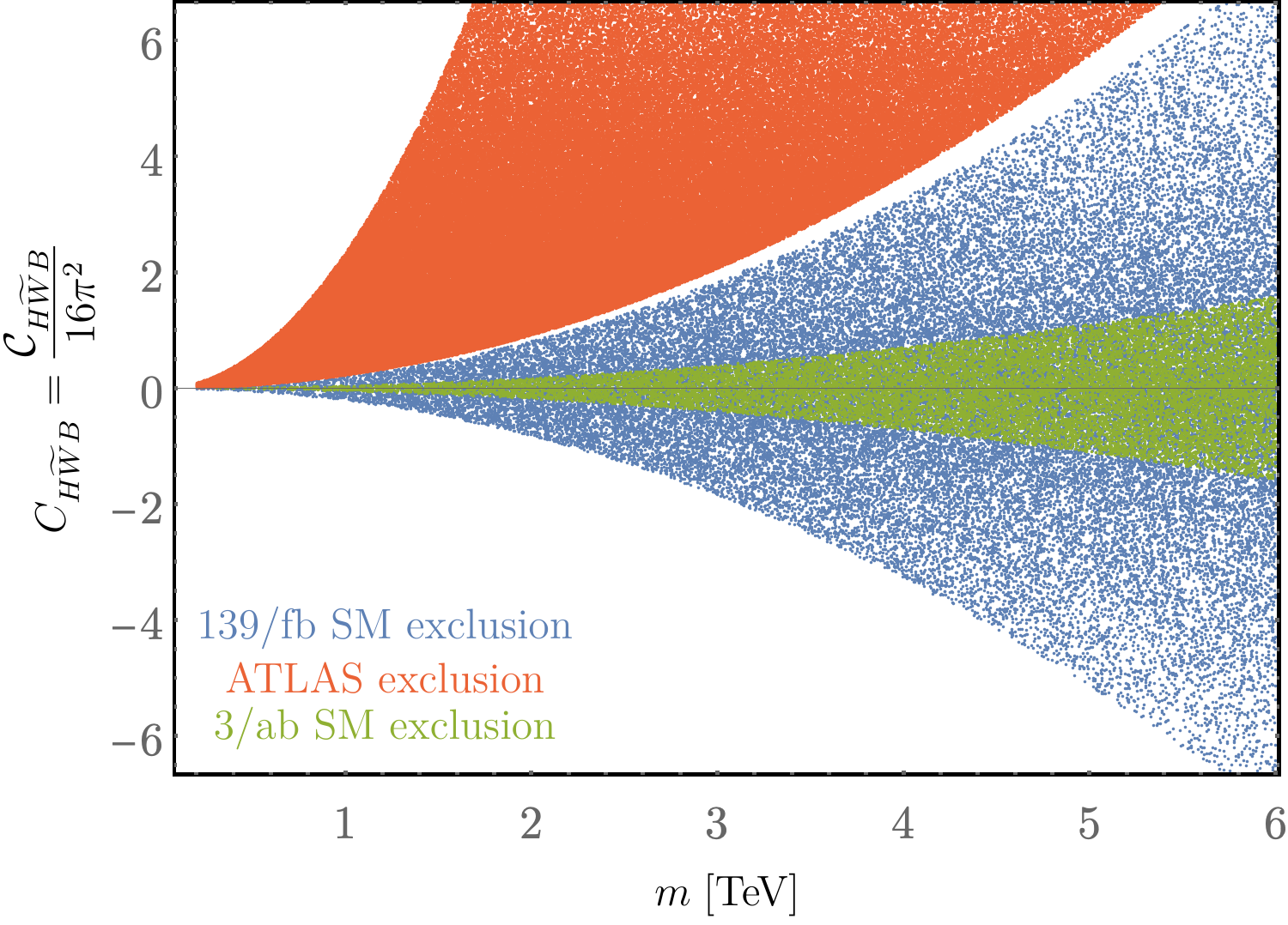
In Fig. 3, we show a scan over the model parameters when contrasted with the parameter constraints of the ATLAS analysis result of Eq. (4). It can be seen that that the large excess in the 95% constraint that is in tension with the SM favours either low mass scales or very large, potentially non-perturbative couplings. Direct searches for vector-like leptons have been discussed in Kumar and Martin 2015 and a HL-LHC direct coverage should be possible up to mass scales of 450 GeV which translates into model thus probing . For such relatively low scales, where the EFT scale is identified with the statistical threshold of a particular analysis, the couplings are still in the strongly-coupled, yet perturbative regime. Such large couplings, can lead to potential tension with other observables that are correlated through our particular model assumption. The constraints outlined in Sec. III.2 are in fact stronger, in particular for the combination of .
Returning to the complementary constraints that can be derived from the diboson, and in particular the analyses, we show the expected sensitivity range to the new physics scenario and its compatibility with the allowed parameter space consistent with the EWPO and Higgs signal strength in Fig. 4†††† †† It is important to note that while generating the EWPO+Higgs data consistent parameter space, the CP violating observables are not included.. We choose three benchmark points (see Tab. 4) and show the 65% and 95% C.L. regions in the plane. There it becomes clear that the searches outlined in the beginning of this work will provide important sensitivity to this particular model class in the future in the direction, which (for our choice of ) is relatively unconstrained by Higgs and EWPO data.


| Fit parameters | Set-1 | Set-2 | Set-3 |
|---|---|---|---|
| (Best fit) | |||
| 1.00 | 1.05 | 0.25 | |
| 0.32 | 0.19 | 0.27 | |
| 1.00 | 0.61 | 0.73 | |
| 0.65 | 1.2 | 0.46 | |
| 0.58 | 0.38 | 0.52 | |
| 1.30 | 0.05 | 1.11 |
V Discussion and Conclusions
The insufficient amount CP violation in the SM to explain the observed matter-anti–matter asymmetry is a clear indication of the presence of new physics beyond the SM. Consequently analyses of CP properties of particle physics interactions are an important part of the current phenomenological program at various energies, reaching up to the current high-energy frontier explored at the LHC. The observation of -related excess by the ATLAS collaboration in the recent Ref. Aad et al. 2020b could be the first indication of the presence of such interactions in the gauge boson-Higgs sectors. Taking inspiration from Ref. Aad et al. 2020b, the focus of this work is two-fold:
- (i)
We motivate a particular UV model class, namely that of vector-like leptons Eq. (13), to provide a minimal and consistent theoretical backdrop to the analysis of Ref. Aad et al. 2020b. We perform a complete matching calculation at one-loop order and demonstrate that all relevant CP-odd EFT deformations of the SM amplitude of diboson (and ) are dominantly captured by the operator. In parallel, at the given order we do not induce , which impacts the analyses of CP-odd observables in (di)boson final states as well, but which is consistent with the SM expectation of given the results of Ref. Aad et al. 2020b. The mass scales of the vector-like lepton scenario that can be directly explored at the LHC Kumar and Martin 2015 constrain the model’s parameters to the strong-coupling, yet perturbative regime. An analysis of electroweak precision and Run-2 Higgs results indicates that the region of the ATLAS excess could be explained by and a significant with some tension given the UV-model’s correlation of CP-even and CP-odd couplings for masses that fall into the HL-LHC kinematic coverage.
- (ii)
The excess observed by ATLAS deserves further scrutiny. We show that diboson analyses, and in particular production will serve as a strong cross check of the excess, in particular because its phenomenology is particularly sensitive to -induced deviations. The analysis suggested in Sec. II.1, will therefore allow the collaborations to directly explain the results of Ref. Aad et al. 2020b as a statistical fluctuation or gather further, strong evidence for a non-SM source of CP violation.
Finally, the correlation of different Wilson coefficients as predicted by our matching calculation motivates additional Higgs-based phenomenology probe that can further constrain or solidify the excess through measurements that target, e.g. in a suitable way Bernlochner et al. 2019 (see also Huang et al. 2020; Cirigliano et al. 2019).
Acknowledgements.
S.D.B. would like to thank Sunando Patra for the clarifications regarding the OptEx package and Anisha for helpful discussions on the statistical analysis. The work of S.D.B. and J.C. is supported by the Science and Engineering Research Board, Government of India, under the agreements SERB/PHY/2016348 (Early Career Research Award) and SERB/PHY/2019501 (MATRICS). C.E. is supported by the UK Science and Technology Facilities Council (STFC) under grants ST/P000746/1 and ST/T000945/1 and by the IPPP Associateship Scheme. M.S. is supported by the STFC under grant ST/P001246/1. P.S. is supported by an STFC studentship under grant ST/T506102/1.Appendix A Wilson Coefficients of the dimension six effective operators in the SILH-like basis
| Operators | Operator Definition | |
|---|---|---|
Appendix B Corrections to the EWPOs from dimension six Warsaw basis operators
The dimension six effective operators may affect the electroweak observables and modify the couplings related to the SM Higgs production and decay. These observables are very precisely measured. Thus any alteration beyond their SM predicted values puts stringent constraints on the WCs associated with those operators.
The electroweak parameters under consideration are
and can be expressed as functions of the electroweak input parameters fine structure constant , mass of boson , and Fermi constant ‡‡‡‡ ‡‡ gets correction from and dimension six operators. In the case of the model of Eq. (13) these two operators are absent, thus we directly impose ..
Here, we capture the additional contributions to the EWPOs, the relevant parameters and couplings, following the prescription suggested in Refs. Dawson and Giardino 2020; Alonso et al. 2014; Brivio et al. 2017, in the presence of the computed dimension six operators in our VLL framework, see Tab. 2. We estimate the contributions to the following parameters based on Refs. Dawson and Giardino 2020; Alonso et al. 2014; Brivio et al. 2017 (we denote the gauge couplings with and , respectively):
- •
and :
(22) (23) respectively.
- •
the Higgs boson mass :
(24) - •
the Weinberg angle ():
(25) - •
the gauge coupling ():
(26) - •
the couplings of fermions to charged gauge bosons:
(27) - •
the mass and width of boson:
respectively,
- •
the couplings of left() and right () chiral fermions to boson:
The total scattering cross section of boson
including the effects of , and , can then be calculated straightforwardly. The partial decay width of the boson into fermions is given by
| (28) |
where is the color charge of the fermions. The change in the partial decay width is computed in a very similar way as done for . Furthermore, the ratios of the changes in partial decays, e.g., , and , and the asymmetries and forward-backward can be recast in terms of changes of the couplings.
References
- Sakharov (1967) A. D. Sakharov, Pisma Zh. Eksp. Teor. Fiz. 5, 32 (1967), [JETP Lett.5,24(1967); Sov. Phys. Usp.34,no.5,392(1991); Usp. Fiz. Nauk161,no.5,61(1991)].
- Aad et al. (2020a) G. Aad et al. (ATLAS), Phys. Rev. Lett. 125, 061802 (2020a), eprint 2004.04545.
- Sirunyan et al. (2020a) A. M. Sirunyan et al. (CMS), Phys. Rev. Lett. 125, 061801 (2020a), eprint 2003.10866.
- Aad et al. (2020b) G. Aad et al. (ATLAS) (2020b), eprint 2006.15458.
- Grzadkowski et al. (2010) B. Grzadkowski, M. Iskrzynski, M. Misiak, and J. Rosiek, JHEP 10, 085 (2010), eprint 1008.4884.
- Arnold et al. (2009) K. Arnold et al., Comput. Phys. Commun. 180, 1661 (2009), eprint 0811.4559.
- Baglio et al. (2014) J. Baglio et al. (2014), eprint 1404.3940.
- Bellm et al. (2016) J. Bellm et al., Eur. Phys. J. C76, 196 (2016), eprint 1512.01178.
- Aad et al. (2011) G. Aad et al. (ATLAS), JHEP 09, 072 (2011), eprint 1106.1592.
- Chatrchyan et al. (2014) S. Chatrchyan et al. (CMS), Phys. Rev. D89, 092005 (2014), eprint 1308.6832.
- Goebel et al. (1981) C. J. Goebel, F. Halzen, and J. P. Leveille, Phys. Rev. D23, 2682 (1981).
- Brodsky and Brown (1982) S. J. Brodsky and R. W. Brown, Phys. Rev. Lett. 49, 966 (1982).
- Brown et al. (1983) R. W. Brown, K. L. Kowalski, and S. J. Brodsky, Phys. Rev. D28, 624 (1983), [Addendum: Phys. Rev.D29,2100(1984)].
- Baur et al. (1993) U. Baur, T. Han, and J. Ohnemus, Phys. Rev. D 48, 5140 (1993), eprint hep-ph/9305314.
- Baur et al. (1994) U. Baur, S. Errede, and G. L. Landsberg, Phys. Rev. D50, 1917 (1994), eprint hep-ph/9402282.
- Han (1995) T. Han, AIP Conf. Proc. 350, 224 (1995), eprint hep-ph/9506286.
- Aihara et al. (1995) H. Aihara et al., pp. 488–546 (1995), eprint hep-ph/9503425.
- Christensen and Duhr (2009) N. D. Christensen and C. Duhr, Comput. Phys. Commun. 180, 1614 (2009), eprint 0806.4194.
- Alloul et al. (2014) A. Alloul, N. D. Christensen, C. Degrande, C. Duhr, and B. Fuks, Comput. Phys. Commun. 185, 2250 (2014), eprint 1310.1921.
- Degrande et al. (2012) C. Degrande, C. Duhr, B. Fuks, D. Grellscheid, O. Mattelaer, and T. Reiter, Comput. Phys. Commun. 183, 1201 (2012), eprint 1108.2040.
- Alwall et al. (2011) J. Alwall, M. Herquet, F. Maltoni, O. Mattelaer, and T. Stelzer, JHEP 06, 128 (2011), eprint 1106.0522.
- de Aquino et al. (2012) P. de Aquino, W. Link, F. Maltoni, O. Mattelaer, and T. Stelzer, Comput. Phys. Commun. 183, 2254 (2012), eprint 1108.2041.
- Alwall et al. (2014) J. Alwall, R. Frederix, S. Frixione, V. Hirschi, F. Maltoni, O. Mattelaer, H. S. Shao, T. Stelzer, P. Torrielli, and M. Zaro, JHEP 07, 079 (2014), eprint 1405.0301.
- Alwall et al. (2007) J. Alwall et al., Comput. Phys. Commun. 176, 300 (2007), eprint hep-ph/0609017.
- Khachatryan et al. (2017) V. Khachatryan et al. (CMS), Phys. Lett. B766, 268 (2017), eprint 1607.06943.
- Aaboud et al. (2019) M. Aaboud et al. (ATLAS), Eur. Phys. J. C79, 884 (2019), eprint 1905.04242.
- Campbell and Ellis (1999) J. M. Campbell and R. K. Ellis, Phys. Rev. D60, 113006 (1999), eprint hep-ph/9905386.
- Campbell et al. (2011) J. M. Campbell, R. K. Ellis, and C. Williams, JHEP 07, 018 (2011), eprint 1105.0020.
- Campbell et al. (2015) J. M. Campbell, R. K. Ellis, and W. T. Giele, Eur. Phys. J. C75, 246 (2015), eprint 1503.06182.
- Boughezal et al. (2017) R. Boughezal, J. M. Campbell, R. K. Ellis, C. Focke, W. Giele, X. Liu, F. Petriello, and C. Williams, Eur. Phys. J. C77, 7 (2017), eprint 1605.08011.
- Campbell and Neumann (2019) J. Campbell and T. Neumann, JHEP 12, 034 (2019), eprint 1909.09117.
- Angelescu and Huang (2020) A. Angelescu and P. Huang (2020), eprint 2006.16532.
- Corbett et al. (2018) T. Corbett, M. J. Dolan, C. Englert, and K. Nordström, Phys. Rev. D 97, 115040 (2018), eprint 1710.07530.
- Das Bakshi et al. (2019) S. Das Bakshi, J. Chakrabortty, and S. K. Patra, Eur. Phys. J. C79, 21 (2019).
- Ellis et al. (2020) S. A. R. Ellis, J. Quevillon, P. N. H. Vuong, T. You, and Z. Zhang (2020), eprint 2006.16260.
- Bélusca-Maïto et al. (2018) H. Bélusca-Maïto, A. Falkowski, D. Fontes, J. C. Romão, and J. a. P. Silva, JHEP 04, 002 (2018), eprint 1710.05563.
- Giudice et al. (2007) G. F. Giudice, C. Grojean, A. Pomarol, and R. Rattazzi, JHEP 06, 045 (2007), eprint hep-ph/0703164.
- Contino et al. (2013) R. Contino, M. Ghezzi, C. Grojean, M. Muhlleitner, and M. Spira, JHEP 07, 035 (2013), eprint 1303.3876.
- Brivio et al. (2017) I. Brivio, Y. Jiang, and M. Trott, JHEP 12, 070 (2017), eprint 1709.06492.
- Dedes et al. (2017) A. Dedes, W. Materkowska, M. Paraskevas, J. Rosiek, and K. Suxho, JHEP 06, 143 (2017), eprint 1704.03888.
- Golden and Randall (1991) M. Golden and L. Randall, Nucl. Phys. B361, 3 (1991).
- Holdom and Terning (1990) B. Holdom and J. Terning, Phys. Lett. B247, 88 (1990).
- Altarelli and Barbieri (1991) G. Altarelli and R. Barbieri, Phys. Lett. B253, 161 (1991).
- Peskin and Takeuchi (1990) M. E. Peskin and T. Takeuchi, Phys. Rev. Lett. 65, 964 (1990).
- Grinstein and Wise (1991) B. Grinstein and M. B. Wise, Phys. Lett. B265, 326 (1991).
- Altarelli et al. (1992) G. Altarelli, R. Barbieri, and S. Jadach, Nucl. Phys. B369, 3 (1992), [Erratum: Nucl. Phys.B376,444(1992)].
- Peskin and Takeuchi (1992) M. E. Peskin and T. Takeuchi, Phys. Rev. D46, 381 (1992).
- Burgess et al. (1994) C. P. Burgess, S. Godfrey, H. Konig, D. London, and I. Maksymyk, Phys. Lett. B326, 276 (1994), eprint hep-ph/9307337.
- Grojean et al. (2013) C. Grojean, E. E. Jenkins, A. V. Manohar, and M. Trott, JHEP 04, 016 (2013), eprint 1301.2588.
- Englert and Spannowsky (2015) C. Englert and M. Spannowsky, Phys. Lett. B740, 8 (2015), eprint 1408.5147.
- Bernlochner et al. (2019) F. U. Bernlochner, C. Englert, C. Hays, K. Lohwasser, H. Mildner, A. Pilkington, D. D. Price, and M. Spannowsky, Phys. Lett. B790, 372 (2019), eprint 1808.06577.
- Englert et al. (2019) C. Englert, G. F. Giudice, A. Greljo, and M. Mccullough, JHEP 09, 041 (2019), eprint 1903.07725.
- Sirunyan et al. (2020b) A. M. Sirunyan et al. (CMS), Eur. Phys. J. C80, 75 (2020b), eprint 1908.06463.
- Dawson and Giardino (2020) S. Dawson and P. P. Giardino, Physical Review D 101 (2020).
- Alonso et al. (2014) R. Alonso, E. E. Jenkins, A. V. Manohar, and M. Trott, JHEP 04, 159 (2014).
- Murphy (2018) C. W. Murphy, Physical Review D 97 (2018).
- Patra (2019) S. Patra, sunandopatra/optex-1.0.0: Wo documentation (2019), URL https://doi.org/10.5281/zenodo.3404311.
- Baak et al. (2014) M. Baak, J. Cúth, J. Haller, A. Hoecker, R. Kogler, K. Mönig, M. Schott, and J. Stelzer, The European Physical Journal C 74 (2014).
- Aad et al. (2016a) G. Aad et al. (ATLAS, CMS), JHEP 08, 045 (2016a), eprint 1606.02266.
- Aad et al. (2016b) G. Aad et al. (ATLAS), Eur. Phys. J. C76, 6 (2016b), eprint 1507.04548.
- Aad et al. (2020c) G. Aad et al. (ATLAS), Phys. Rev. D 101, 012002 (2020c), eprint 1909.02845.
- Aad et al. (2020d) G. Aad et al. (ATLAS) (2020d), eprint 2004.03447.
- Aad et al. (2020e) G. Aad et al. (ATLAS) (2020e), eprint 2005.05382.
- Aad et al. (2019a) G. Aad et al. (ATLAS) (2019a), eprint ATLAS-CONF-2019-028.
- Aad et al. (2020f) G. Aad et al. (ATLAS) (2020f), eprint ATLAS-CONF-2020-007.
- Aaboud et al. (2018a) M. Aaboud et al. (ATLAS), Phys. Rev. D97, 072003 (2018a), eprint 1712.08891.
- Aaboud et al. (2018b) M. Aaboud et al. (ATLAS), Phys. Lett. B 784, 173 (2018b), eprint 1806.00425.
- Aad et al. (2019b) G. Aad et al. (ATLAS), Phys. Lett. B 798, 134949 (2019b), eprint 1903.10052.
- Sirunyan et al. (2019) A. M. Sirunyan et al. (CMS), Eur. Phys. J. C 79, 421 (2019), eprint 1809.10733.
- Sirunyan et al. (2020c) A. M. Sirunyan et al. (CMS), JHEP 03, 131 (2020c), eprint 1912.01662.
- Kumar and Martin (2015) N. Kumar and S. P. Martin, Phys. Rev. D 92, 115018 (2015), eprint 1510.03456.
- Huang et al. (2020) D. Huang, A. P. Morais, and R. Santos (2020), eprint 2009.09228.
- Cirigliano et al. (2019) V. Cirigliano, A. Crivellin, W. Dekens, J. de Vries, M. Hoferichter, and E. Mereghetti, Phys. Rev. Lett. 123, 051801 (2019), eprint 1903.03625.