Metaclusters for the Full Control of Mechanical Waves

Can the cluster be invisible, in the sense that there is no scattered wave? Setting ${\bf A}$ to zero implies

Hence $B_{\alpha}=0$, and therefore $t_{\alpha}=0$, meaning there are no scatterers, the null solution. We conclude that the inverse scattering cluster scheme does not provide a useful route to invisibility or cloaking.

Let us assume that the $N$ scatterers lie on the circle of radius $R$ at $\theta_{\beta}=2\pi\beta/N$. We consider $\bf A$ corresponding to each of the modes $e^{\mathrm{i}m\theta}$, $m\in\mathbb{Z}$, so that $||{\bf A}||^{2}=1$ and $E\leq 1$ with $E\ll 1$ indicating the desired scattering mode is well approximated. The results of numerical experimentation are as follows. For small $kR$ relative to $N$, $E$ is small for modes $m=0,\pm 1,\ldots,\frac{N-1}{2}$ if $N>1$ is odd, and for modes $m=0,\pm 1,\ldots,\frac{N-2}{2}$ if $N$ is even, with $E\approx 0.5$ for $m=\pm\frac{N}{2}$. The accuracy diminishes as $kR$ increases. In other words, for small $kR$ the $N$ unit eigenvalues of $\bf P$ correspond to modes $m=0,\pm 1,\ldots,\frac{N-1}{2}$ if $N>1$ is odd, with analogous association for $N$ even. Since the modes are multiply degenerate (all of eigenvalue unity) it follows that any linear combination of these modes is an eigenvector.

We now assume that the scatterers are distributed in a square but finite lattice. The lattice is $M\times M\equiv N$ with lattice spacing $a$. For instance, with $M=3$ and $ka=1$ we find that the 9 eigenvectors of $\bf P$ of eigenvalue $+1$ span the space $\Omega_{4}\equiv\{e^{\mathrm{i}m\theta},\ m=0,\pm 1,\ldots,\pm 4\}$. This result is arrived at by inspecting the error $E$ for each mode, and noting that it is small, on the order of $1e-4$ typically, while higher modes have error of approximately unity.

However, for the same $ka=1$ but the larger lattice with $M=4$ $(N=16)$ we find that the nontrivial eigenspace is $\Omega_{5}\bigcup\Omega_{6,10}$ where $\Omega_{6,10}$ is a five dimensional subspace formed from $\{e^{\mathrm{i}m\theta},\ m=\pm 6,\ldots,\pm 10\}$.

Numerical experiments on matrix ${\bf P}$ for different spatial configurations of the clusters show that for large and moderate $kR$ there are exactly $N$ eigenvalues of ${\bf P}$ with values close to 1. For large $kR$, the corresponding eigenvectors (i.e. patterns of scattering modes of the cluster) are highly irregular and sensitive to both $kR$ and scatterers positions (while the number of eigenvalues of value $1$ equals $N$). For $kR_{c}\approx 0.5$ and smaller, where $R_{c}$ is the characteristic size of the cluster, the eigenvalues of ${\bf P}$ begin to differ and assume values other than 1. For $kR_{c}\ll 1$ the number of nonzero eigenvalues reduces and low order scattering patterns are preferred.

Some general remarks on the number of scatterers ($N$) and scattering properties of the cluster can be formulated as follows. The larger $N$, the larger number of cluster modes, thus more complex scattering patterns can be reproduced accurately. Large number of scatterers in the cluster, on the other hand, may result in overconstraining the minimization problem and lack of locally or globally passive solutions. For moderate $kR_{c}$ typically the number of regular patterns (eigenvectors of ${\bf P}$) is similar to $N$, while more degenerate patterns and/or smaller number of similar eigenvalues ($\approx 1$) are observed for large or small $kR_{c}$.

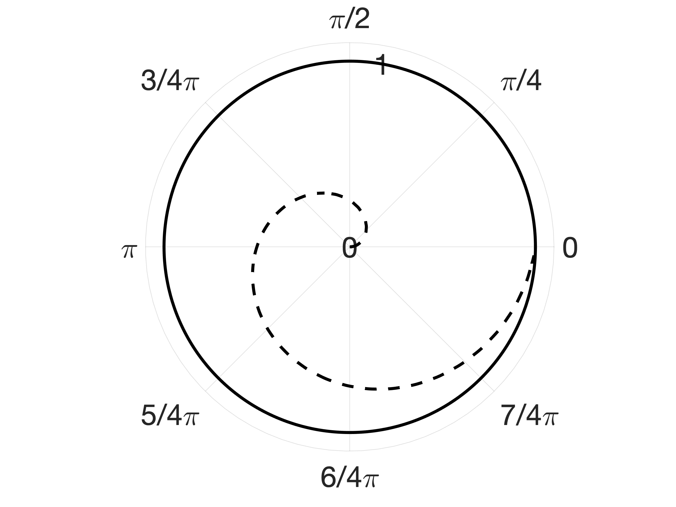
Uni-directional scattering in the direction $\theta=\theta_{0}$ corresponds to

A bi-directional scattering pattern is of the form $f(\theta)=C_{0}\delta(\theta-\theta_{0})+C_{1}\delta(\theta-\theta_{1})$. We consider patterns that are symmetric or anti-symmetric about the $x-$direction $(\theta=0)$, corresponding to $\theta_{1}=-\theta_{0}$ and $C_{1}=\pm C_{0}$. We may choose $C_{0}=1$ with no loss in generality, and define

Examples of the uni- and bi-directional scattering patterns are shown in Figs. 1(a) and 1(b). .

Odd-pole patterns have $\bar{p}$ scattering lobes directing energy towards that preferential directions. The odd-pole scattering pattern and the corresponding $A_{n}$ coefficients are given as

where $\theta^{\prime}=\theta\,\text{mod}\,2\pi$ is used to ensure that $f(\theta)$ is a $2\pi-$periodic function.

A vortex generates uniform constant amplitude pattern with angle-dependent linearly changing phase behavior. The corresponding formulas for the vortex of order $\bar{p}\in\mathbb{Z}$ are

Directional characteristics of amplitudes and phases for the vortex pattern are shown in Fig. 1(e).

Scattering patterns obtained for selected cluster topologies are shown in Fig. 2. Very good agreement between the desired patterns of Fig. 1 can be seen, proving the effectiveness of the design procedure. However, some of the corresponding impedances - computed using the inverse approach of Sec. III.3 - are active, hence require energy supply. We next analyze and adopt the inverse procedure for seeking only locally passive solutions.

Our design objective is the set of point impedances $\{t_{\alpha},\,\alpha=1,\ldots,N\}$. We aim at fulfilling the local passivity condition, Eq. (8b). Define

then Eq. (6) becomes $u_{\alpha}=p_{\alpha}+s_{\alpha}$, $\alpha=1,\ldots,N$. Consider plane wave incidence $\psi_{0}({\bm{r}})=p_{0}e^{\mathrm{i}{\bm{k}}\cdot{\bm{r}}}$, for some wavenumber $\bm{k}$. There is a further degree of freedom that has not been used. This could be considered as the amplitude and phase of the incident wave, i.e. the complex number $p_{0}$. Alternatively, if we fix $p_{0}=1$, then there is a similar degree of freedom in how we normalize the far field pattern function $f(\theta)$. This has the effect of scaling $\bf A$ and hence $\bf B$ by a complex number. This scaling redefines $p_{\alpha}$ but has no effect on $s_{\alpha}$ of (31).

Therefore, with no loss in generality we assume the incident wave has unit amplitude,

and rewrite Eq. (6), the solution of the inverse problem, to incorporate this added degree of freedom, as

Here the complex number $z$ defines the scaling of the pattern function, which goes as $z^{-1}$. The important point is that $z$ can be chosen arbitrarily; in particular, we use it as an optimization parameter. The fact that the pattern function amplitude is inversely proportional to $|z|$ for unit amplitude incident wave suggests that smaller $|z|$ is preferred for maximizing efficiency of energy conversion.

The optimization problem is as follows: given the $N$ complex numbers $p_{\alpha}$ associated with the incident wave and the $N$ complex numbers $s_{\alpha}$ associated with the point sources, find $z$ of Eq. (33) that ensures $\operatorname{Im}u_{\alpha}\leq 0$ for all $\alpha$. If this can be achieved then the optimal solution is the one with minimum value of $|z|$, ensuring maximum amplitude for the pattern function. It might not be possible using the single complex number $z$ to obtain all of the complex numbers $u_{\alpha}$ in the negative imaginary half-plane. If this is not achievable in practical examples then the constraint may be relaxed, for instance, to minimize the maximum instance of positive $\operatorname{Im}u_{\alpha}$. Then the ”nearest” passive configuration can be identified by setting $\operatorname{Im}u_{\alpha}$ to zero for those particles with positive $\operatorname{Im}u_{\alpha}$. Another alternative could be based on condition (8a), i.e. when the metacluster is globally passive - meaning that the net energy supplied to the cluster non-positive.

In cases where the search procedure for $t_{\alpha}$ failed to find locally passive metaclusters, a rigid rotation was applied to the cluster (equivalent to changing the incidence angle) and the search was repeated.

Numerical experimentation shows there are metacluster configurations for which the inverse impedance solutions are all passive. Examples of the uni- and bi-directional scattering patterns for a square lattice metacluster are shown in Figure 2. More detailed investigations show that - for instance - a square array with lattice parameter $a$ designed to direct a wave incident from the $\theta=\pi$ direction into a scattered wave preferentially directed toward $\theta=3/4\pi$ has totally passive solutions for $1.9\leq ka\leq 2.8$. The optimal passive admittances $t_{\alpha}^{-1}$ are frequency dependent, with values at the end of the passive interval shown in Table 1. The associated optimal scattering patterns are shown in Figure 3. In all examples we take $a=1$ and $D=1$.

The examples in Figure 3 and Table 1 are based on the value of $z$ in (33) for which the largest value of $\operatorname{Im}t_{\alpha}^{-1}$ is zero. This optimizes the passive array in terms of its efficiency in converting the incident energy into a directed far field pattern. The metacluster dissipates wave energy but in a way that is most efficient among all passive options. For the cluster shown in Fig. 3, the values of the efficiency parameter $\eta$ of Eq. (17) are $\eta_{ka=1.9}=0.60$ and $\eta_{ka=2.8}=0.35$.

Similarly, Fig. 4 shows a passive optimal $2\times 2$ metacluster that converts the incident plane wave into a symmetric bi-directional pattern. Although the metacluster scattering pattern roughly approximates the desired far field function, all admittances are purely real indicating no dissipation in the system. Consequently, the energy efficiency for this cluster is optimal, $\eta=1$.

Further experimentation shows that obtained optimal solutions are very sensitive to the scatterers’ positions and impedances. Also, requirements of symmetric clusters are overconstrained, most often resulting in at least one active particle, especially for large number of particles $N$.

Analogously to the previous search, we look for optimal passive clusters capable of generating a scattering tripole. Figure 5 shows the target and the actual scattering patterns for the tripole obtained for a square $2\times 2$ cluster of scatterers. The optimal positions and admittances of the scatterers are shown in Table 3. The admittances have nearly the same passive damping properties. The corresponding displacement field pattern generated by the metacluster is shown in Fig. 5. The energy conversion efficiency is $\eta=0.17$.

Figure 6 shows a metacluster designed for generating a pentapole pattern. The cluster consists of a circular arrangement of five scatterers with optimal positions and impedances listed in Table 4. Clearly, the cluster is locally passive. It is important to note that this metacluster setup, resulting in nearly perfect pentapole (red dashed line in Fig. 6(a)), has been obtained accidentally when looking for the vortex-type scattering pattern (different than the pentapole pattern, see black solid line in Fig. 6(a)). The latter is a consequence of relaxing the requirement of enforcing the target phase of the scattered field and indicates that much more complex scattering patterns that are still locally passive may be obtained for desired amplitude-only rather than amplitude-and-phase target fields. This cluster also displays high energy conversion efficiency with $\eta=0.84$.

Finally, we present a locally passive metacluster capable of transforming the incident wavefield into the first-order vortex, $\bar{p}=1$, as shown in Fig. 7. It can be seen from Fig. 7(a) that despite the amplitude pattern is not perfectly preserved, the phase behavior (Fig. 7(b)) recovers the linearly-dependent angular characteristic of the vortex. Figures 7(c) and 7(d) show displacements and phases of the wavefields generated by the metacluster. It is worth noting that this relatively complex scattering pattern is obtained by only four passive impedances. The cluster efficiency is $\eta=0.14$ for this setup, being a consequence of moderate damping in all scatterers.

References

- Jin et al. (2019a) Y. Jin, B. Djafari-Rouhani, and D. Torrent, Nanophotonics 8, 685 (2019a).
- Engheta and Ziolkowski (2006) N. Engheta and R. W. Ziolkowski, Metamaterials: physics and engineering explorations (John Wiley & Sons, 2006).
- Deymier (2013) P. A. Deymier, Acoustic metamaterials and phononic crystals, Vol. 173 (Springer Science & Business Media, 2013).
- Yu et al. (2011) N. Yu, P. Genevet, M. A. Kats, F. Aieta, J.-P. Tetienne, F. Capasso, and Z. Gaburro, science 334, 333 (2011).
- Kildishev et al. (2013) A. V. Kildishev, A. Boltasseva, and V. M. Shalaev, Science 339 (2013).
- Yu and Capasso (2014) N. Yu and F. Capasso, Nature materials 13, 139 (2014).
- Ra’di et al. (2017) Y. Ra’di, D. L. Sounas, and A. Alù, Physical review letters 119, 067404 (2017).
- Wong and Eleftheriades (2018) A. M. Wong and G. V. Eleftheriades, Physical Review X 8, 011036 (2018).
- Torrent (2018) D. Torrent, Physical Review B 98, 060101 (2018).
- Packo et al. (2019) P. Packo, A. N. Norris, and D. Torrent, Physical Review Applied 11, 014023 (2019).
- Popov et al. (2019a) V. Popov, F. Boust, and S. N. Burokur, Physical Review Applied 11, 024074 (2019a).
- Popov et al. (2019b) V. Popov, M. Yakovleva, F. Boust, J.-L. Pelouard, F. Pardo, and S. N. Burokur, Physical Review Applied 11, 044054 (2019b).
- Jin et al. (2019b) Y. Jin, X. Fang, Y. Li, and D. Torrent, Physical Review Applied 11, 011004 (2019b).
- Ni et al. (2019) H. Ni, X. Fang, Z. Hou, Y. Li, and B. Assouar, Physical Review B 100, 104104 (2019).
- He et al. (2020) J. He, X. Jiang, D. Ta, and W. Wang, Applied Physics Letters 117, 091901 (2020).
- Martin (2006) P. A. Martin, Multiple scattering: interaction of time-harmonic waves with N obstacles, 107 (Cambridge University Press, 2006).
- Torrent et al. (2013) D. Torrent, D. Mayou, and J. Sánchez-Dehesa, Physical Review B 87, 115143 (2013).
- Norris and Vemula (1995) A. Norris and C. Vemula, Journal of sound and vibration 181, 115 (1995).
- Evans and Porter. (2007) D. V. Evans and R. Porter., Journal of Engineering Mathematics 58, 317 (2007).
- Abramowitz and Stegun (1974) M. Abramowitz and I. Stegun, Handbook of Mathematical Functions with Formulas, Graphs, and Mathematical Tables (Dover, New York, 1974).