ECG Classification with a Convolutional Recurrent Neural Network

Since only 27 out of the 111 diagnoses found in the dataset were scored in the challenge, we grouped all non-scored diagnoses into one “negative” class. Furthermore, three pairs of diagnoses were considered as equivalent in the challenge. We mapped all recordings labelled SVPB or VPB to PAC or PVC respectively, since their ECG patterns are similar enough not to confuse the network during training. However, since the QRS duration is different between CRBB and RBBB by definition, we did not combine these two diagnoses into one class.

We excluded leads with redundant information, namely leads III, aVR, aVL and aVF. Since the dataset includes recordings sampled at 257 Hz, 500 Hz and 1000 Hz, we resampled the data to the lowest of the three, 257 Hz. Since some of the very long recordings (30 minutes) have a significant drift, we applied a high pass filter with a cutoff at 0.5 Hz to all signals. We then split the data into training (80%) and validation (20%) [hereafter referred to as “local validation”] sets stratified by dataset and the least common label found in each recording. Finally, each lead was normalized by the standard deviation over the training data. To augment the data and increase model generalization capabilities, a random offset was sampled for the beginning of the first window every time an ECG recording was presented to the network.

We selected a network architecture combining convolutional and recurrent blocks (see Figure 1). The convolutional block was used to extract features while the recurrent block was used to handle signals of varying length. The convolutional block has 15 convolutional layers that are split into five mini-blocks. Each mini-block has three convolutional layers, each with a rectified linear unit (ReLU) activation function. The first two convolutions in the mini-block have a kernel size of 3 and stride 1, while the last has a kernel size of 24 and stride 2, excluding the very last convolution layer, which has a kernel size of 48. A dropout layer with a dropout rate of 10% is added after each mini-block. In addition, each mini-block has skip connections. In all mini-blocks except the first, the skip connection is from the very beginning of the block, until before the last convolutional layer in the block. The first block is slightly different with the skip connections starting after the first convolution, but before the activation. This is to ensure that the input and output of the skip connection have the same dimensions. The convolutional block is concluded with a global average pooling layer which produces a feature vector for each window. These feature vectors are then fed into the recurrent block, composed of a bi-directional gated recurrent unit (GRU), with dropout for both the inputs and the recurrent state, followed by a ReLU activation, a dropout on the outputs and concluding with an attention layer with context [5]. The recurrent block produces one feature vector for the whole signal that is normalized over the batch and finally a fully connected layer with a sigmoid activation function produces the non-exclusive class probabilities. The final model was trained for 350 epochs, with a batch size of 8 recordings and the loss function was binary cross-entropy. Recordings with similar durations were grouped together to limit zero padding. The biggest batch size that did not exceed the hardware limitations during training was 8. The epoch with the highest local validation score was selected as the final model. The choice of optimizer was considered as a hyperparameter (see Section 2.5 and Section 3.2). The model was implemented in TensorFlow 2.2.0.

To boost the performance of the model and to ensure that the offset of the input signal does not play a decisive role in the decision, we applied test time augmentation (TTA). To perform TTA, we applied ten different offsets to the input signal. A prediction was then made on each of these ECG signals. The mean of the resulting prediction probabilities was then thresholded to get the final decision.

Several hyperparameters of the network were optimized. To increase efficiency, the data was downsampled to 100 Hz and recordings longer than 200 s were excluded during hyperparameter optimization. Where possible, the model with the highest local validation score was selected.

Optimizer: The first step was to find a suitable optimizer to minimize the binary cross-entropy loss. The tested optimizers were: Stochastic Gradient Descent (SGD), Adam [6], AMSGrad [7], and Nesterov Adam (Nadam) [8]. The optimizers were executed for 150 epochs with their default parameters in TensorFlow 2.2.0 on the full dataset resampled at 500 Hz optimizing the network from [4] with an added global average pooling layer at the end of the convolutional block.

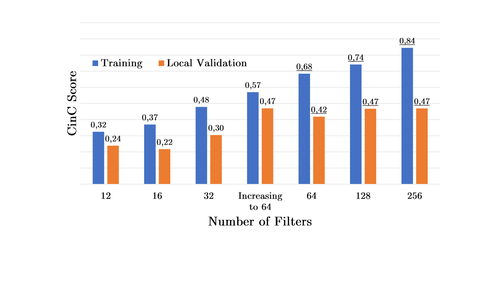
Number of Filters: The number of filters in [4] was constant for all layers (12 filters per layer). We performed a grid search of this hyperparameter with the values of 12, 16, 32, 64, 128, and 256. Since models with 64 or more filters per layer exceeded the hardware limitations set by the challenge, a model with 16 filters in the first mini-block, 32 filters in the next two and 64 in the last two, which did not exceed the hardware limitations, was also tested.

Dropout: Two different dropout rates were used: one for the convolutional block ($d_{c}$) and one for the recurrent block ($d_{r}$). A grid search was run over these parameters. The range of the convolutional dropout was $d_{c}\in\left[0,0.2\right]$ with a 0.1 increment. The tested dense/recurrent dropout rates were $d_{c}\in\{0.2,0.5,0.7\}$.

Decision Threshold: Decision threshold optimization was performed after training by simply taking the prediction probabilities of the model on the local validation set and compute the challenge metric with different thresholds ranging from 0 to 1 with 0.1 increment.

Other hyperparameters tested either did not have an effect on the overall score (halving the kernel sizes to account for lower sampling rate, increasing number of mini-blocks by one), a negative effect (changing which layers within each mini-block would be followed by a dropout), or exceeded hardware limitations (e.g., additional GRU layer, doubling GRU number of hidden units). Moreover, additional methods to alleviate class imbalance were tested: focal loss [9], oversampling, MLSMOTE [10], and an ensemble of binary and multi-label deep models. However, none of them successfully balanced the label distribution nor resulted in a higher local nor hidden validation score.

Optimizer: The training score over each epoch of each optimizer can be seen in Figure 2. Nadam with the default parameters showed the most promise, but it was unstable. Therefore, we reduced its learning rate to $10^{-4}$. The local validation score showed a similar progression over epochs.

Number of Filters: Training and local validation scores are depicted in Figure 3. For a fair comparison, the scores are shown from the same epoch of all models. With more filters, the local validation performance goes up until it plateaus at 128 filters while the training performance goes up, a clear sign of overfitting. The models whose scores are underlined exceeded the hardware limitations. Note also that the local validation performance of the model with increasing number of filters with depth has a higher local validation score but lower training score than the equivalent model with constant number of filters, a sign of a more generalizable model.

Dropout: The local validation scores obtained were in the range $\left[0.38,0.47\right]$. The combination of dropout rates with the highest local validation score of was $d_{c}=0.1$ and $d_{r}=0.7$. All scores mentioned are from the same epoch.

Decision Threshold: The best threshold for the model with the hyperparameters described in Section 2.3 was 0.3 and yielded a local validation score of 0.573, a 0.027 improvement from the model with the default threshold (0.5).

Finally, applying TTA resulted in an increase in the range of $\left[0.0002,0.02\right]$ depending on the model. The network was tested with and without skip connections, adding the skip connections resulted in an 0.1 increase in score.

The model with optimized hyperparameters yielded a score of 0.451 on the training set and 0.522 on the local validation set which increased to 0.546 with addition of TTA and up to 0.573 with the optimized threshold as well. The model with optimized hyperparameters and TTA was submitted with a threshold of 0.5 and with the optimized threshold of 0.3. The obtained hidden validation scores were 0.313 and 0.511 respectively. The model with a threshold of 0.3 was selected for testing on the final hidden test set resulting in a final test score of 0.167.

References

- [1] Benjamin EJ, Muntner P, Alonso A, et al. Heart Disease and Stroke Statistics – 2019 Update: a Report From the American Heart Association. Circulation 2019;139:e56–e528.
- [2] Goldberger AL, Amaral LA, Glass L, et al. PhysioBank, PhysioToolkit, and PhysioNet: Components of a New Research Resource for Complex Physiologic Signals. Circulation 2000;101(23):e215–e220.
- [3] Perez Alday EA, Gu A, Shah A, et al. Classification of 12-lead ECGs: the PhysioNet/Computing in Cardiology Challenge 2020. Physiol Meas 2020;(In Press).
- [4] Chen TM, Huang CH, Shih ES, Hu YF, Hwang MJ. Detection and Classification of Cardiac Arrhythmias by a Challenge-Best Deep Learning Neural Network Model. Iscience 2020;23(3):100886.
- [5] Yang Z, Yang D, Dyer C, et al. Hierarchical Attention Networks for Document Classification. In Proceedings of the 2016 Conference of the North American Chapter of the Association for Computational Linguistics: Human Language Technologies. 2016; 1480–1489.
- [6] Kingma DP, Ba J. Adam: A Method for Stochastic Optimization. arXiv preprint arXiv14126980 2017;https://arxiv.org/abs/1412.6980.
- [7] Reddi SJ, Kale S, Kumar S. On the Convergence of Adam and Beyond. In Proceedings of the International Conference on Learning Representations (ICLR). 2018; 1–23.
- [8] Dozat T. Incorporating Nesterov Momentum into Adam. Proceedings of 4th International Conference on Learning Representations 2016;Workshop Track.
- [9] Lin TY, Goyal P, Girshick R, et al. Focal Loss for Dense Object Detection. In Proceedings of the IEEE international conference on computer vision. 2017; 2980–2988.
- [10] Charte F, Rivera AJ, del Jesus MJ, Herrera F. MLSMOTE: Approaching Imbalanced Multilabel Learning Through Synthetic Instance Generation. Knowledge Based Systems 2015;89:385–397.
Halla Sigurthorsdottir
Rue Jaquet-Droz 1, Neuchâtel, NE, Switzerland
halla.sigurthorsdottir@csem.ch