August 11, 2026
Efficient Scaling and Moving Techniques for Spectral Methods in Unbounded Domains
Abstract
When using Laguerre and Hermite spectral methods to numerically solve PDEs in unbounded domains, the number of collocation points assigned inside the region of interest is often insufficient, particularly when the region is expanded or translated to safely capture the unknown solution. Simply increasing the number of collocation points cannot ensure a fast convergence to spectral accuracy. In this paper, we propose a scaling technique and a moving technique to adaptively cluster enough collocation points in a region of interest in order to achieve a fast spectral convergence. Our scaling algorithm employs an indicator in the frequency domain that is used to determine when scaling is needed and informs the tuning of a scaling factor to redistribute collocation points to adapt to the diffusive behavior of the solution. Our moving technique adopts an exterior-error indicator and moves the collocation points to capture the translation. Both frequency and exterior-error indicators are defined using only the numerical solutions. We apply our methods to a number of different models, including diffusive and moving Fermi-Dirac distributions and nonlinear Dirac solitary waves, and demonstrate recovery of spectral convergence for time-dependent simulations. Performance comparison in solving a linear parabolic problem shows that our frequency scaling algorithm outperforms the existing scaling approaches. We also show our frequency scaling technique is able to track the blowup of average cell sizes in a model for cell proliferation.
AMS subject classifications: 65M70; 65F35; 65M50; 33C45; 41A05;
Keywords: Unbounded domain; Scaling; Moving mesh; Laguerre function; Hermite function; Blowup; Spectral method
1 Introduction
Many scientific models described by PDEs with blowup solutions are set in unbounded domains. For example, in many models of cellular proliferation, a “blowup” in which the average size of a population of cells becomes uncontrolled and diverges over many generations of growth is possible [3]. The conditions under which blowup occurs is difficult to determine analytically [1] but has been explored numerically [22]. However, numerically tracking “blowup” behavior over long times is extremely difficult, as it requires solving the problem in a truly unbounded domain to capture the diverging mean size. There are many other problems where it is desirable to find a numerical solution in an unbounded domain, including the stability of solitary waves arising from the nonlinear Dirac equation [14, 6] and diffusion in a parabolic system [10].
Considerable progress has recently been made in spectral methods for solving PDEs in unbounded domains [16]. Among the existing spectral methods, the direct approach that is typically used is based on orthogonal basis functions defined on infinite intervals, e.g., the Hermite and Laguerre spectral methods [5, 7, 20]. It has been demonstrated that the performance of these spectral methods can be greatly improved when a proper coordinate scaling is used [19, 16]. However, it is not clear how to systematically perform the scaling, especially when transient behavior arises. A Hermite spectral method with time dependent scaling has been proposed for parabolic problems by introducing a time dependent scaling factor to meet the coercive condition [10]. Nonetheless, the form of and related parameters are chosen based on specified knowledge of parabolic models and thus cannot be easily generalized to other problems.
Motivated by the success of adaptive methods in bounded domains [13, 18, 9], we propose two indicators to adaptively allocate a sufficient number of collocation points to represent the unknown solution in the region of interest. The first indicator, designed for matching the diffusion of unknown solutions, extracts the frequency-space information of intermediate numerical solutions and isolates its high frequency components. This frequency indicator not only provides a lower bound for the interpolation error, but also measures the decay of the derivatives of the reference solution as . By tuning a scaling factor in our proposed scaling technique, the frequency indicator can be maintained at a low level. However, the translation of unknown solutions may also amplify the frequency indicator and thus may result in larger errors for excessive scaling. To accommodate this scenario, a second, exterior-error indicator is used to calculate an upper bound for the error in the exterior domain, allowing one to capture translation via moving collocation points. Accordingly, for problems that may involve both translation and diffusion in unbounded domains, the above two indicators are combined in a “first moving then scaling” approach. Numerical experiments demonstrate their ability to recover a faster spectral convergence for time-dependent solutions.
The remainder of this paper is organized as follows. Section 2 introduces the frequency indicator, connects it to the approximation error, and proposes the frequency-dependent scaling technique for diffusion. Section 3 proposes the exterior-error-dependent moving technique for translating problems. We then combine, in Section 4, the above two approaches to solve time-dependent problems involving both diffusion and translation. Section 5 compares the frequency-dependent scaling with a time-dependent scaling proposed in [10] for solving parabolic systems. In Section 6, we apply the frequency-dependent scaling method to a PDE model describing structured cell populations to track blowup behavior. Finally, we summarize our approaches and make concluding remarks in Section 7.
2 Frequency-dependent scaling
In this section, we formulate a scaling technique by first extracting frequency domain information on the evolution of numerical solutions, the pseudo-code of which is presented in Alg. 1. Following Guo et al. [7], the discussion utilizes the generalized Laguerre polynomials which are mutually orthogonal on the half-line with weight function
| (2.1) |
The generalized Laguerre polynomials of degree are denoted by and reduce to the usual Laguerre polynomials when . In this work, we regard to be the scaling factor, and seek a time-dependent spectral approximation of on . Henceforth, for notational simplicity, the -dependence will usually be omitted.
For any , the spectral approximation using the interpolation operator is
| (2.2) |
where the coefficients can be computed by using e.g., the Laguerre-Gauss collocation points ,
| (2.3) |
where is the expansion order (i.e., collocation points or basis functions), is the inner product, denotes the corresponding weight for collocation point , and
| (2.4) |
Let be the nonuniformly weighted Sobolev space. For any integer , its seminorm and norm are defined by
| (2.5) |
For any with integer , there is a well-known interpolation error estimate when using Laguerre-Gauss collocation points [7]:
| (2.6) |
Here, denotes a generic positive constant which does not depend on , , , or any function. This error estimate is a crucial element in the formal development and successful implementation of the proposed scaling and moving techniques.
When the scaling factor is updated from to , the collocation points, weights and norms are updated according to
| (2.7) |
The expansion coefficients can then be estimated through Eq. (2.3) where we may use the approximation (2.2): . This procedure constitutes the scale subroutine in Lines 9 and 17 of Alg. 1.
To implement the scaling technique, one needs to determine when to apply it and how to choose a new scaling factor such that spectral accuracy can be kept for a prescribed expansion of order . To this end, we propose a frequency indicator acting on the numerical solution :
| (2.8) |
which measures the contribution of the highest-frequency components to the -norm of . The subroutine frequency_indicator in Lines 3, 6, 10, and 18 of Alg. 1 calculates this contribution in which we choose in view of the often-used -rule [8, 12].
If the frequency indicator increases over time, the contribution of high frequency components to the numerical solution increases, indicating that the numerical solution is decaying more slowly in and that we need to adjust the scaling factor to enlarge the computational domain demarcated by the smallest and largest collocation point positions. In Line 7 of Alg. 1, is the threshold at some time . If the value of the frequency indicator of the current numerical solution , then we consider scaling. The parameter is usually chosen to be slightly larger than to prevent the frequency indicator becoming too large without invoking scaling.
However, the if condition is only a necessary condition. Only after we enter the while loop in Line 11 will we perform scaling, which aims to ensure that the frequency indicator will not increase after scaling. Actually, this while loop tries to minimize by geometrically shrinking the scaling factor ( in Line 16 is the common ratio) to ensure sufficient scaling since is a lower bound for the numerical error, as shown in Eq. (2.11). A more continuous adjustment is preferred by setting to be slightly less than , which may also prevent over-shrinking of the scaling factor within one single time step. Henceforth, we will choose and . Moreover, at the initial time , we also ensure the frequency indicator is small enough by choosing a suitable initial scaling factor.
In this work, the generalized Laguerre polynomials with are used and the relative -error
| (2.9) |
is used to measure the quality of the spectral approximation to the reference solution . We always use the most updated scaling factor to calculate the above error.
Example 1.
We use the spreading Fermi-Dirac distribution
| (2.10) |
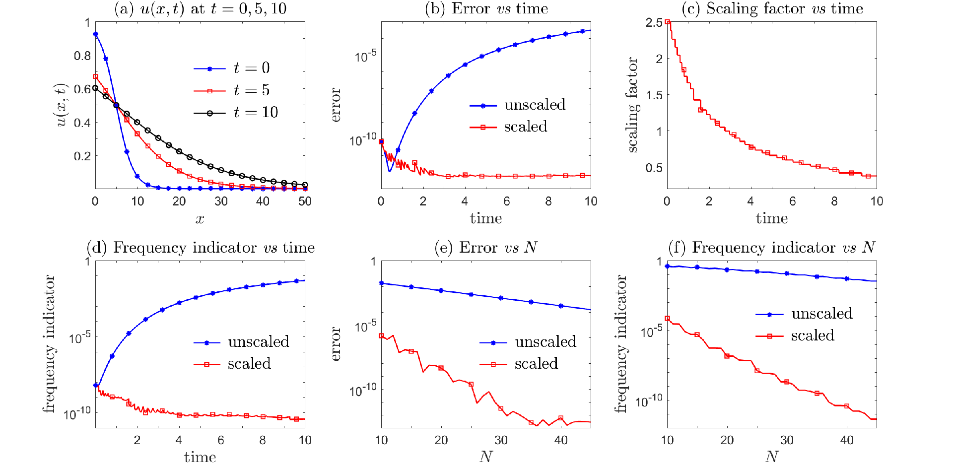
to test the performance of the scaling algorithm 1. It can be readily verified that the reference solution expands over time as shown in Fig. 1(a). The proposed frequency-dependent scaling with effectively maintains the relative error under up until time whereas the error for the corresponding unscaled solution rapidly grows to over (see Fig. 1(b)). We also plot, as evolves, the history of the scaling factor and frequency indicator in Figs. 1(c) and 1(d), respectively. It is clear that the frequency indicator increases for the unscaled solution as time evolves and that time-dependent scaling is required to preserve the accuracy. The proposed frequency-dependent scaling technique detects the error and shrinks the scaling factor in order to enlarge the computational domain in accordance with the expansion of the reference solution. The spectral convergence as a function of the expansion order can be also recovered by Alg. 1. The errors at the final time, for the scaled and unscaled approach, are displayed in Fig. 1(e). The final scaling factors at are for , respectively, having all decreased from the common initial scaling factor of 2.5. Figs. 1(e, f) show very similar and expected behavior of the frequency indicator and error as a function of . Since the error and the frequency indicators behave similarly across time (see Figs. 1(b, d)), we also expect them to behave similarly with . These similarities suggest a possible connection between the error and the frequency indicator.
The success of the scaling algorithm 1 is rooted in the connection between the frequency indicator (2.8) and the evolution of the information embedded in the numerical solutions. There are two reasons to use a frequency indicator. First, starting from Eq. (2.8) with and a sufficiently large expansion order , we have
| (2.11) | ||||
which provides an estimate to the lower bound of . Minimizing in Alg. 1 may reduce the lower bound of the interpolation error. Moreover, a straightforward application of the interpolation error estimator (2.6) to the two terms in the numerator of Eq. (2.11) yields
| (2.12) |
where the constant . Thus, we find
| (2.13) |
implying that , we may choose a sufficiently large such that .
Secondly, the frequency indicator can be used to measure the decay of the reference solution’s derivatives as tends to infinity. According to inequality (2.13), if is fixed, a larger implies a larger . In particular, given (e.g., ), if
| (2.15) |
and
| (2.16) |
In other words, as the frequency indicator increases, the norm of becomes larger than that of , implying scaling is indeed needed to enlarge the computational domain because is the dominant component of . Here, denotes the characteristic function on a set . The verification of inequality (2.16) can be finished by contradiction. If (2.16) does not hold, we would have
which would contradict the inequality (2.15). Intuitively, basis functions of higher degree decay more slowly than those of lower degree, so an increase in the frequency indicator implies slower decay at infinity. This slower spatial decay as time increases requires using a larger computational domain which is achieved by decreasing . In practice, we can also obtain good numerical results using although no theoretical result like the above observation is guaranteed since is not defined.
3 Exterior-error-dependent moving
Dynamics in unbounded domains can be much richer than the simple diffusive behavior successfully captured by our frequency-dependent scaling. Other physical mechanisms may induce, for example, translations (Examples 2 and 3) and emerging oscillations (Example 4). A purely scaling approach fails in these cases.
In this section, we develop an exterior-error-dependent moving method that will be able to resolve a solution’s decay in an undetermined exterior domain . Alg. 2 presents the pseudo-code of our exterior-error-dependent moving technique. In the algorithm, we first need to determine the time-dependent left-end point . Next, we move the spectral basis accordingly so that the spectral approximation for an unknown function in (denoted by ) maintains accuracy. To implement this procedure, we adopt an exterior-error indicator:
| (3.1) |
which measures the proportion of the norm inside a prescribed unbounded domain .
The subroutine exterior_error_indicator in Lines 5, 8, and 13 of Alg. 2 calculates . Here, following the often-used -rule [8, 12], we choose from the collocation points in the exterior domain .
Intuitively, if moves rightward in time, such as the moving Fermi-Dirac distribution in Example 2, the spectral approximation at large distances may deteriorate and the exterior-error indicator will increase. Consequently, the moving mechanism is triggered in Line 9 of Alg. 2, and completed by updating the left end point in Line 11. Thus, the starting point of the spectral approximation also moves rightward with time to capture the translation.
The displacement is determined by the move subroutine in Line 10, where is the smallest integer satisfying , is the minimum displacement, is the maximum displacement, and represents the threshold of the increase in the exterior-error indicator that we can tolerate. In practice, should be based on a prior knowledge of the maximum translation speed of the function . We usually choose to prevent the exterior-error indicator from becoming too large without invoking moving. The move subroutine also generates from .
Example 2.
In this example, we consider the moving Fermi-Dirac distribution
| (3.2) |
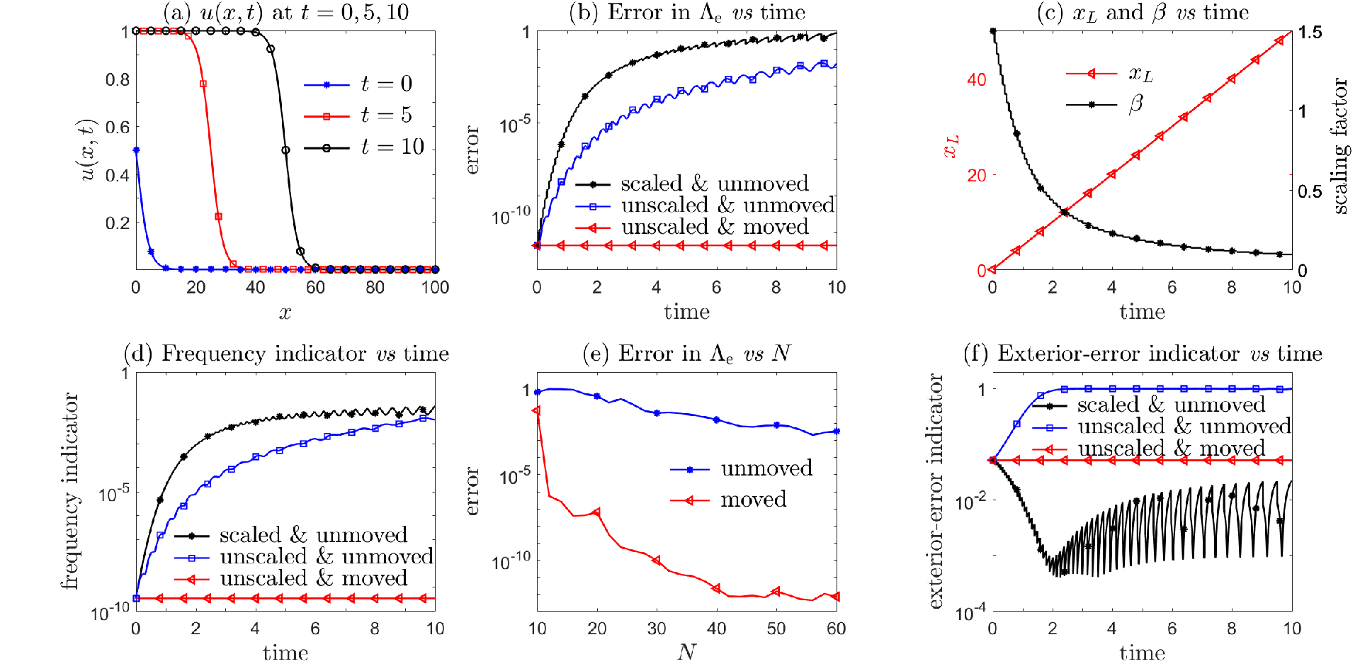
which travels to the right at a speed of without any shape change (see Fig. 2(a)). The scaling algorithm 1, equipped with the same parameters that worked well for the diffusive Fermi-Dirac distribution in Example 1, fails to capture the translation. In fact, the errors of the scaled solutions are larger than those of unscaled ones as shown in Fig. 2(b). It seems that the decrease of the scaling factor (black curve with asterisks in Fig. 2(c)) cannot compensate for the increase in the frequency indicator (black curve with asterisks in Fig. 2(d)). In other words, the scaling algorithm 1 mistakes translation as diffusion and performs excessive scaling. In contrast, the exterior-error-dependent moving algorithm 2 with , and succeeds in producing a much more accurate approximation to the moving Fermi-Dirac distribution given by Eq. (3.2) in the exterior domain , with errors kept under up to time (red curve with left-pointing triangles in Fig. 2(b)). The moving technique recovers a faster spectral convergence with respect to the expansion order as shown in Fig. 2(e).
During the moving process, the exterior-error indicator is well controlled (red curve with left-pointing triangles in Fig. 2(f)) and the left-end point of the exterior domain closely tracks the uniform linear motion (red curve with left-pointing triangles in Fig. 2(c)). The exterior-error indicator monotonically increases for the unscaled and unmoved solutions (blue curve with squares in Fig. 2(f)) and oscillates rapidly for the scaled and unmoved solutions (black curve with asterisks in Fig. 2(f)). Moreover, the similarity between the relative error and frequency indicator as a function of time is again confirmed by comparing Fig. 2(d) to Fig. 2(b), thus providing strong evidence for the effectiveness of using the frequency indicator (2.8). Spectral convergence in is clearly observed for the moving spectral method in Fig. 2(e) while the error decays slowly with for the unmoved spectral method.
Example 3.
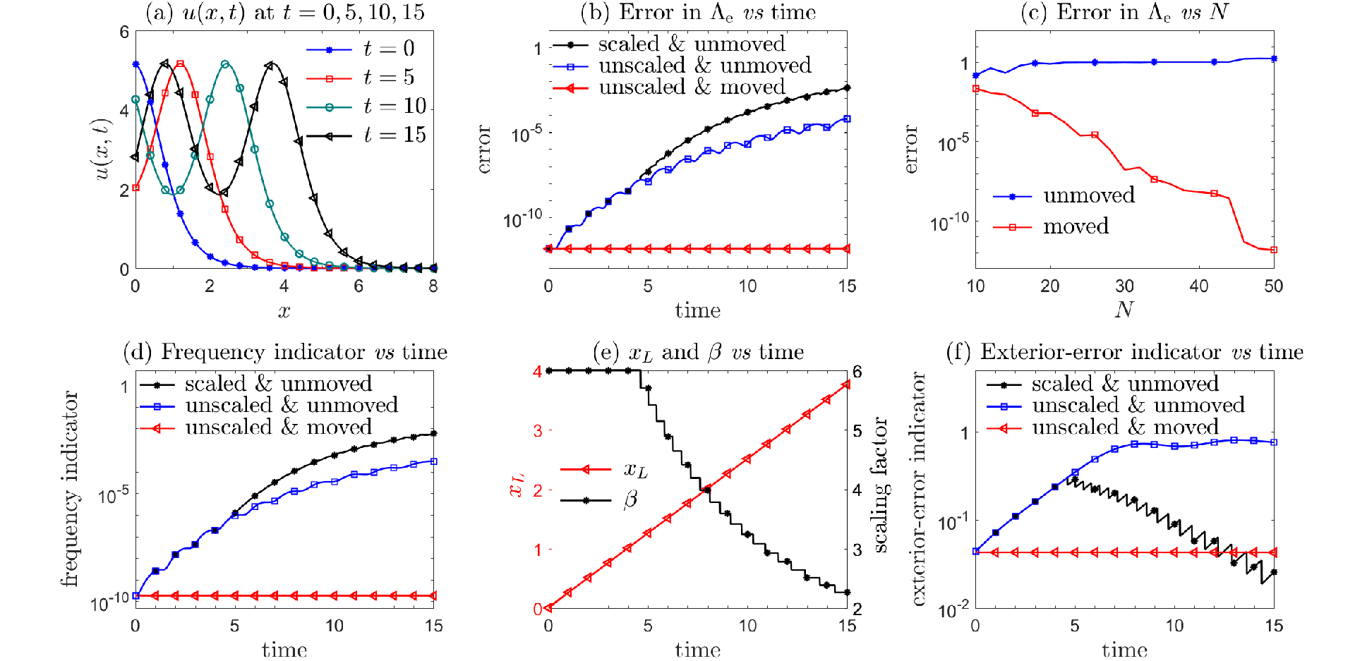
Another class of dynamical systems are described by solitons or solitary waves in which nonlinearities and dispersion counteract. While solitons have been well-studied, there has been recent interest in nonlinear Dirac solitary waves as they emerge naturally in many physical systems [6]. Stability of the nonlinear Dirac solitary waves on the whole line and its connection to the multi-hump structure is a challenging topic of research [14, 24, 2]. In this example, we approximate a right-moving two-hump solitary wave, the explicit form of which is given in [15] with , , , and . The reference solutions are plotted in Fig. 3(a).
Numerical results are displayed in Fig. 3 where we set , , . It can be readily observed there that the exterior-error-dependent moving algorithm 2 produces much more accurate solutions with errors kept under until the final time (red curve with left-pointing triangles in Fig. 3(b)). The moving algorithm also recovers a faster spectral convergence with respect to the expansion order (see Fig. 3(c)). The scaling-only algorithm 1 fails to maintain the accuracy (black curve with asterisks in Fig. 3(b)). The similarity between the relative error and frequency indicator is again confirmed by comparing Fig. 3(d) to Fig. 3(b).
In Examples 2 and 3, the exterior-error indicator (3.1) efficiently guides us in finding an such that the moved spectral approximation retains accuracy in the resulting exterior domain. The accuracy arises from the fact that the exterior-error indicator is related to the upper bound of the error for asymptotically large . If we assume a large indicator with , then the upper bound for the error in is larger than the upper bound for the error in :
The solution in the interior domain is not approximated by the basis functions used to approximate the solution in the exterior domain. Obstacles to designing moving mesh methods in unbounded domains include the construction of an interior numerical solution and its consistent coupling with the exterior spectral approximation. More on these issues will be illustrated in Example 4.
Example 4.
Let us approximate the following function in :
| (3.3) |
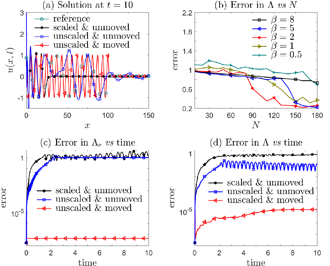
which represents a wave with period traveling to the right with speed 10 and exponentially decaying at infinity. The reference solution is plotted by the green curve with circles in Fig. 4(a), which coincides with the red curve with left-pointing triangles hat approximates seperately in and using different basis funcitons. As shown by the blue curve with squares in Fig. 4(a), applying a Laguerre spectral approximation with and in fails to accurately approximate . This failure arises because more oscillations emerge from and translate to as time evolves. Specifically, at , the reference solution possesses extrema while any Laguerre spectral approximation (2.2) with can have at most extrema, implying that the approximation is doomed to fail since all oscillations cannot be captured. Simply increasing the number of basis functions does little to help, even with different scaling factors as shown in Fig. 4(b). The ineffectiveness of increasing is mainly due to the presence of oscillatory components with significantly different frequencies in each of the two different domains. As shown by the black curves with asterisks in Figs. 4(a, c, d), the scaling technique is also doomed to fail because it totally neglects this scale difference and only adjusts the scaling factor to redistribute collocation points.
We propose a divide-and-conquer strategy to address Example 4 that can be implemented by applying two subroutines, within each time step. The first step is to use the exterior-error-dependent moving algorithm 2 to determine the exterior spectral approximation for the exponential decay component of the reference solution. The second step is to introduce a new spectral approximation in the remaining bounded interior domain for the left-side oscillating component. The full numerical solution in the half-line is constructed from concatenating the solution in the exterior domain to the one in the interior domain .
Fig. 4(c) plots the error in the exterior domain against time and shows that the errors of of the moved solution with , , and are kept under up to time (red curve with left-pointing triangles), confirming that the Laguerre spectral approximation is accurate in the exterior domain. In fact, the numerical values of obtained by the moving algorithm 2 are consistent with the expected value of as shown in Eq. (3.3). Coupling the exterior solution with a spectral approximation using Chebyshev polynomials in the interior domain, we find a combined numerical solution with total relative error under up to (red curves with left-pointing triangles in Figs. 4(a, d)) using total basis functions. By contrast, Fig. 4(b) shows that the errors for direct refinement using are larger than .
It must be pointed out that when solving PDEs in unbounded domains, we may need information about the solution in the exterior domain to construct the interior numerical solution. Further discussion on this point can be found in Example 6.
4 Spectral methods incorporating both scaling and moving
For problems that involve both translation and diffusion in unbounded domains, we need to incorporate both the moving and scaling procedures. Since the scaling algorithm 1 may mistake translation for diffusion and trigger an inappropriate scaling as shown in Examples 2 and 3, we propose a “first moving then scaling” algorithm. The associated pseudo-code is described in Alg. 3. A direct application of Alg. 3 to Example 1 recovers exactly the same results as Alg. 1 since the moving procedure is not invoked. When Alg. 3 is applied to Examples 2 and 3, it gives the same results as Alg. 2 since the scaling mechanism is not triggered. That is, the combined moving-scaling algorithm 3 can deal with both translation-only and diffusion-only problems since it can distinguish translation from diffusion.
Alg. 3 can be extended to unbounded domains in multiple dimensions in a dimension-by-dimension manner by using the tensor product of one-dimensional basis functions. For example, consider the two-dimensional spectral approximation
| (4.1) |
in where and . We choose the exterior-error indicator in -dimension to be
| (4.2) | ||||
| (4.3) |
Similarly, gives the exterior-error indicator in -dimension. Accordingly, we use to judge the if statement in Line 10 of Alg. 3. If satisfied, then the move subroutine in Line 11 will move the solution in -direction via . Simultaneously, we use to determine the shift in the -direction.
To allow scaling in -direction, the corresponding frequency indicator can be defined as
| (4.4) |
where and are the expansion orders in the -, -directions, respectively. Similarly, we define to be the frequency indicator in -direction. We first keep fixed and use to evaluate the if statement in Line 16 for scaling. If scaling in -direction is needed, then the while loop in Line 20 will update the scaling factor to . Simultaneously, we fix and use to update the scaling factor in the -direction to . After that, the scaling factors for time are set to and .
Example 5.
We will investigate the performance of Alg. 3 in a two-dimensional unbounded domain by considering the function
| (4.5) |
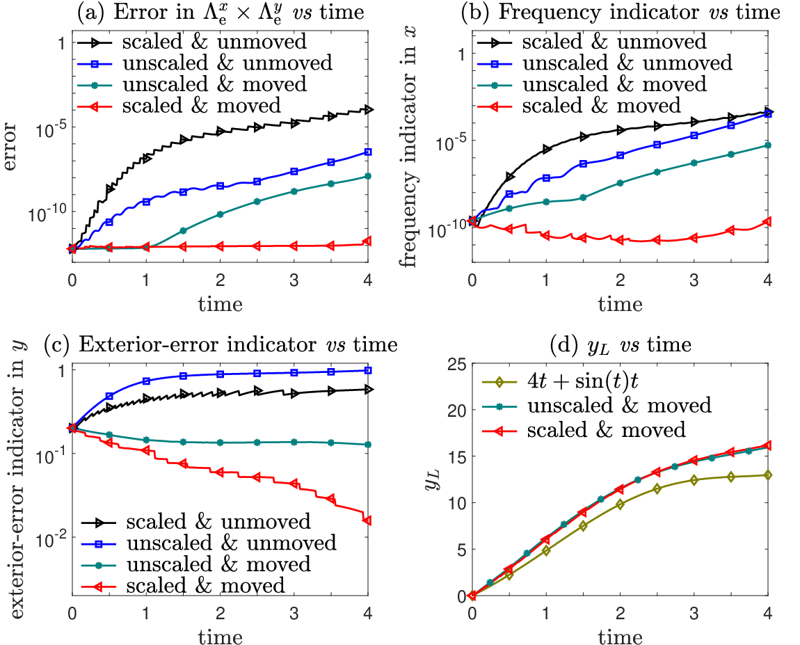
which displays both advective and diffusive behavior. This function exhibits oscillations in space from the factor , an exponential decay, and a translation to infinity with time-varying velocity . The numerical results shown in Fig. 5 are generated using a time step , the same parameters in the -, - directions, and , , , .
As expected, only the combined scaling-moving algorithm 3 keeps the errors in the exterior domain under (up to the final time ), as shown by the error curves in Fig. 5(a). This accuracy is achieved because the corresponding frequency indicator and exterior-error indicator are controlled by our “first moving then scaling” techniques, see e.g., in Fig. 5(b) and in Fig. 5(c).
Although the moving algorithm 2 may accurately capture the function near the left end of the exterior domain, the resulting exterior-error indicator does not stay low enough to preserve accuracy in the exterior domain , as shown by the green curves with asterisks in Figs. 5(a, c, d). The moving algorithm neglects the diffusion and thus uses an improper (smaller) and . The right choice for these two variables depends on proper scaling for the diffusion, revealing why we need to update in Line 7 of Alg. 3 after scaling. That is, the moving determines while the scaling determines , making it necessary to combine moving with scaling.
As we have mentioned in Example 4, numerically solving evolving PDEs in unbounded domains requires both the interior solution in and the exterior solution in after applying the divide-and-conquer strategy. When using the moving-scaling algorithm 3 to march the solution from to , if the moving mechanism is not triggered (i.e., is unchanged), then the interior and exterior solutions can be updated individually in the normal way. If it is triggered, extra steps are needed to approximate the solution in the enlarged interior domain since after running Line 12 of Alg. 3.
In the next Example, we will test the ability of Alg. 3 to solve a one-dimensional PDE where we will use the intermediate (unmoved) exterior solution (obtained immediately after running Line 8) to interpolate the required function values in .
Example 6.
We solve the following first-order PDE
| (4.6) |
with initial data and Dirichlet boundary condition . The analytical solution is a moving and diffusive Fermi-Dirac distribution: , which travels rightward to infinity at a speed of . A simple numerical scheme for evolving Eq. (4.6) is employed here for testing the performance of Alg. 3 within the divide-and-conquer strategy.
Specifically, we adopt the Laguerre spectral approximation (2.2) in the exterior domain, the first order backward finite difference method in the interior domain, and the second order improved Euler scheme in time. We use a nonuniform mesh, e.g., Gauss-Lobatto points, to avoid possible poor resolution in the tiny interior domain at short times. For , a uniform mesh with spacing is used so new grid points in can be easily added. The other parameters were set to , , , and .
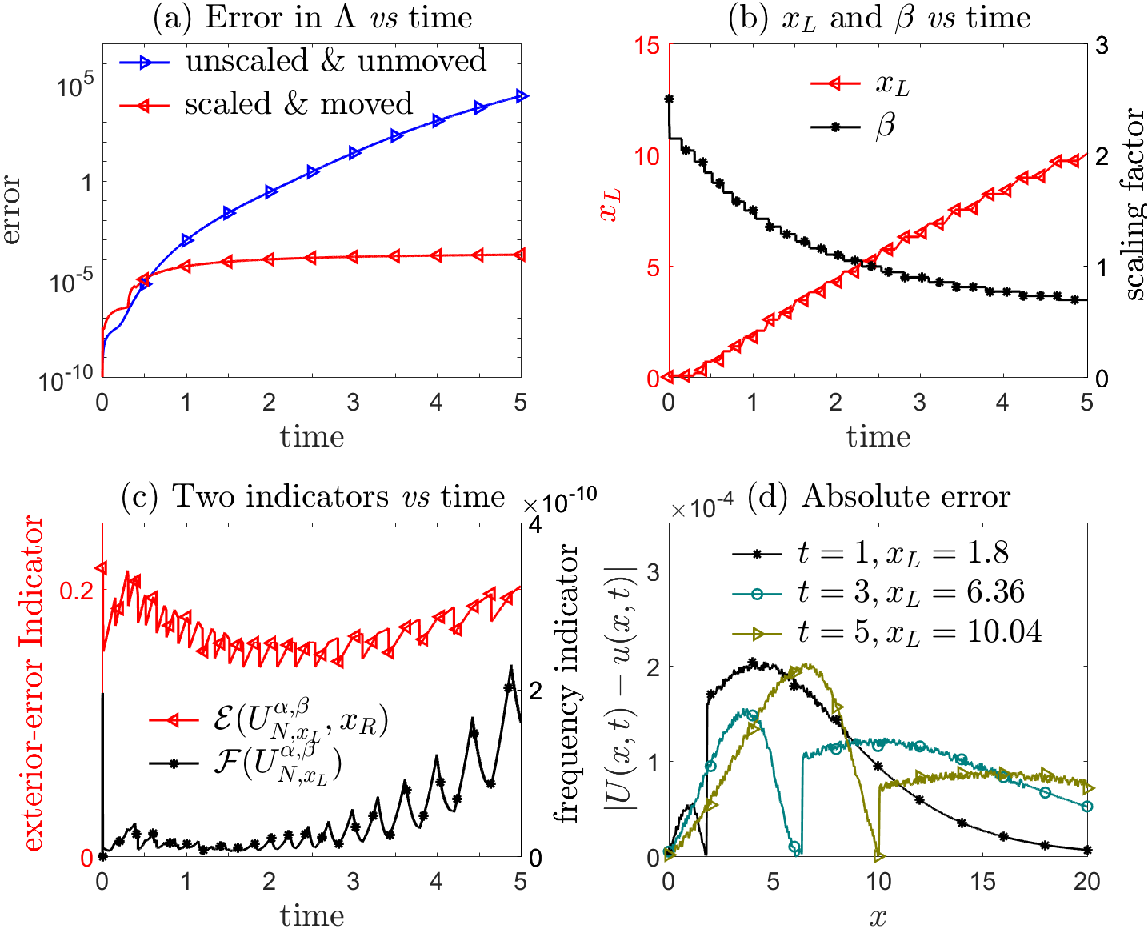
The results summarized in Fig. 6 clearly show that, up to the final time , the proposed divide-and-conquer strategy maintains the errors in the whole domain under (red curve with left-pointing triangles in Fig. 6(a)). Alg. 3 succeeds in capturing the translation, as shown by the red curve with left-pointing triangles in Fig. 6(b), thus determining the exterior domain . Without this strategy, a straightforward use of the Laguerre spectral approximation in leads to huge errors as indicated by the blue curve with right-pointing triangles in Fig. 6(a).
Fig. 6(c) shows that the frequency indicator is always kept under as shown by the black curve with asterisks, a sufficiently small lower error bound for scaling, by continually shrinking the scaling factor shown as the black curve with asterisks in Fig. 6(b). The exterior-error indicator is always maintained around as shown by the red curve with left-pointing triangles in Fig. 6(c), which implies the error in divided by the error in is almost unchanged, ensuring small errors at infinity. Fig. 6(d) plots at different times ( and denote the numerical and analytical solution, respectively). There is a clear divide near arising from the different numerical treatments between the interior and exterior domains.
5 Performance comparison in solving parabolic PDEs
We now apply the frequency-dependent scaling algorithm 1 to solve
| (5.1) |
in , and compare our results with those obtained with the time-dependent scaling method developed in [10]. First, we need to generalize our scaling approach from to by using scaled Hermite polynomials, denoted by , which are mutually orthogonal under the weight function (). Similarly, we use to denote the scaling factor and the frequency indicator defined in Eq. (2.8) still serves as a lower bound for the interpolation error.
We use a standard Galerkin Hermite spectral method to find a solution in satisfying the initial condition and
| (5.2) |
where denotes the corresponding scaled Hermite functions and is the conventional inner product in space. The Galerkin discretization (5.2) is stable in the sense that
| (5.3) |
is strictly positive and can be controlled by . By contrast, a time-dependent scaling factor:
| (5.4) |
was taken in [10] to fix the instability of the Petrov–Galerkin discretization by tuning the parameters and .
Example 7.
We apply the frequency-dependent scaling algorithm 1 to Example 6.1 in [10]. In order to facilitate comparison, we also adopt the same second order-accurate Crank-Nicholson scheme to march Eq. (5.2), and the same errors and to measure the accuracy. Table 1 presents the numerical errors with different time steps and expansion orders where the second-order accuracy in time and the spectral convergence in space are clearly demonstrated. Table 2 compares the errors without scaling to those obtained using the scaling algorithm 1 and the time-dependent scaling method in [10] on the same mesh. Both scaling methods produce much more accurate numerical results but the proposed frequency-dependent scaling keeps the errors around or below , outperforming the time-dependent scaling of [10].
The scaling factor adjusted adaptively by the frequency indicator (2.8) takes on the value at for all choices of time steps shown in Table 2 whereas the time-dependent scaling factor in [10] decreases to at (Eq. 5.4). The smaller scaling factor arises from the stability requirement , an initial value of , and using in Eq. 5.4 [10], and prevents the error from decreasing when the time step is refined from to (see the third column of Table 2). There is no accuracy improvement without scaling when the timestep is decreased as shown in the second column of Table 2 where a scaling factor is fixed to . Regardless of what time step is used in the unscaled method, the error experiences a sudden increase across , rising from below to about , as it fails to capture the diffusion. A similar observation was shown in Table 6.1 of [10].
| Time step | Order | Order | |||
|---|---|---|---|---|---|
| 25 | 2.500e-04 | 2.182e-04 | |||
| 2.499e-07 | -2.000 | 2.227e-06 | 1.991 | ||
| 2.500e-09 | -2.000 | 2.227e-08 | -2.000 | ||
| 2.555e-10 | -1.991 | 2.350e-10 | -1.977 | ||
| 2.203e-04 | 1.619e-04 | ||||
| 2.189e-07 | 4.335e-08 | ||||
| 1.353e-09 | 8.880e-09 | ||||
| 4.840e-11 | 6.183e-11 |
| Time step | No scaling | Time-dependent scaling in [10] | Frequency-dependent scaling in Alg. 1 |
|---|---|---|---|
| 1/250 | 3.969e-04 | 2.598e-06 | 3.998e-07 |
| 1/1000 | 3.910e-04 | 1.189e-06 | 2.503e-08 |
| 1/4000 | 3.390e-04 | 1.117e-06 | 2.085e-09 |
| 1/16000 | 3.390e-04 | 1.117e-06 | 1.381e-09 |
6 Applications to structured cell population models
One example of an application requiring the solution of PDEs in an unbounded domain is the structured population models that track populations of cells endowed with attributes such as their size. The standard sizer-timer model for the density of cells with age near and size near is formulated in [11], and generalizations to include stochasticity in growth rate is studied in [17, 4]. Here we address a continuum model describing a stochastic model for cell populations [21]:
| (6.1) |
where describes the density of cells with respect to age and size at time , is the mean growth rate of an individual cell and is the variance of stochasticity in the growth rate, i.e., , for an individual cell. The fluctuating growth rate manifests itself as a diffusive term. The right-hand-side of Eq. (6.1) represents cell division occurring with division rate . Dirichlet boundary conditions are imposed at , , and at , if we assume that there are no cells of infinite size. More importantly, the boundary condition at should account for two daughter cells (one of size and one of size ) from the binary fission of a mother cell of size :
| (6.2) |
where is the differential division rate representing the rate that a cell of age and size gives birth to a daughter cell of size . Integrating over the daughter cell’s size , and satisfy , reflecting cell number conservation. Finally, to maintain biomass conservation during division, . The prefactor 2 in Eq. (6.2) indicates that a cell of size gives birth to one daughter cell of size and another of size .
The nonlocal boundary condition (6.2) for cell proliferation plays an essential role in depicting how cell division affects the cell population size and age structure, and presents a major obstacle in numerical computation as the integration is taken in the unbounded domain . Another numerical challenge arises from a possible “blow-up” behavior in which
| (6.3) |
Whether blowup can occur is of biological interest [3, 22] and has been predicted within certain cell proliferation models (6.1) under specific conditions [3].
Existing numerical methods such as the finite volume method in [22] typically truncate the unbounded domain into a bounded domain and therefore cannot accurately capture long time blowup behavior of . The need for numerical solutions in the unbounded domain for Eqs. (6.1) and (6.2) is thus evident. We apply the scaling technique built in to Alg. 1 only in -dimension for tracking the increasing , considering the age distribution is often presumed to be stable since no cell could live too long without division. A standard two-dimensional pseudo-spectral method with the generalized Laguerre functions are used in -space, coupled with a third-order TVD Runge-Kutta time discretization in .
Example 8.
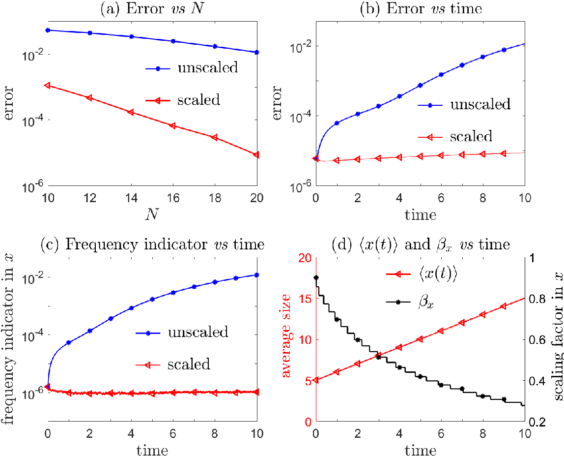
We solve Eqs. (6.1) and (6.2) with , , , . These parameters leads to the analytic solution , which produces the mean size . This result shows that the average size is unbounded as it grows linearly in time and thus, for general cases, requires proper scaling in -dimension. We adopt the same expansion order in both size - and age -dimensions. For the nonlocal boundary condition given in Eq. (6.2), we also use Laguerre-Robatto collocation points in each dimension to perform the numerical integration.
Fig. 7 presents the numerical results with the initial scaling factors and a timestep of . We observe that the frequency-dependent scaling algorithm 1 in -dimension shows a faster spectral convergence with than that of the unscaled algorithm (see Fig. 7(a)). That is, both the sizer-timer model (6.1) in unbounded domain and the nonlocal boundary condition (6.2) are well resolved by the Laguerre spectral approximation with frequency-dependent scaling. When fixing , the unscaled numerical solution experiences an error growth to till for using inappropriate scaling factors, whereas the error of the scaled solution is less than (see Fig. 7(b)). The frequency indicator in the -dimension is kept around (red curve with left-pointing triangles in Fig. 7(c)) by continuously shrinking the scaling factor from to for tracking the blowup (black curve with asterisks in Fig. 7(d)). The average size of the scaled solution behaves almost exactly like and the value at is (see red curve with left-pointing triangles in Fig. 7(d)). Note that the scaling in -dimension will really not be triggered even when we apply the scaling algorithm for both - and -dimensions.
7 Summary and Conclusions
The key to making spectral approximations in unbounded domains more efficient is to allocate collocation points in an economical manner such that crucial regimes of unknown solutions can be resolved accurately. This is essentially an adaptive numerical method for PDEs in unbounded domains, for which there are very few studies compared with its bounded-domain counterpart. Using the standard language of adaptive methods, the proposed scaling technique based on the frequency indicator can be regarded as -adaptivity to redistribute collocation points via adjusting the scaling factor, while the proposed moving technique based on the exterior-error indicator is similar to -adaptivity to add collocation points in the interior subdomain. Both indicators utilize only the numerical solution and do not require any a prior knowledge of unknown solutions. The frequency indicator can be also used in a refinement technique [23] which corresponds to the -adaptivity, useful for time-dependent problems with oscillations at infinity.
Acknowledgments
MX and TC acknowledge support from the National Science Foundation through grant DMS-1814364 and the Army Research Office through grant W911NF-18-1-0345. SS acknowledges the financial support from the National Natural Science Foundation of China (Nos. 11822102, 11421101), Beijing Academy of Artificial Intelligence (BAAI) and the computational resource provided by High-performance Computing Platform of Peking University.
References
- [1] E. Bernard, M. Doumic, and P. Gabriel, Cyclic asymptotic behaviour of a population reproducing by fission into two equal parts, Kinet. Relat. Mod., 12 (2019), pp. 551–571.
- [2] N. Boussaid and A. Comech, Nonlinear Dirac Equation: Spectral Stability of Solitary Waves, American Mathematical Society, 2019.
- [3] S. Burov and D. Kessler, Effective potential for cellular size control, Bull. Am. Phys. Soc., 63 (2018).
- [4] H. Caswell, Sensitivity analysis of the stochastic growth rate: three extensions, Australian & New Zealand Journal of Statistics, 47 (2005), pp. 75–85.
- [5] O. Coulaud, D. Funaro, and O. Kavian, Laguerre spectral approximation of elliptic problems in exterior domains, Comput. Methods Appl. Mech. Engrg., 80 (1990), pp. 451–458.
- [6] J. Cuevas–Maraver, P. G. Kevrekidis, A. Saxena, A. Comech, and R. Lan, Stability of solitary waves and vortices in a 2d nonlinear Dirac model, Phys. Rev. Lett., 116 (2016), p. 214101.
- [7] B. Y. GUO, L. L. Wang, and Z. Q. Wang, Generalized Laguerre interpolation and pseudospectral method for unbounded domains, SIAM J. Numer. Anal., 43 (2006), pp. 2567–2589.
- [8] T. Y. Hou and R. Li, Computing nearly singular solutions using pseudo-spectral methods, J. Comput. Phys., 226 (2007), pp. 379–397.
- [9] R. Li, T. Tang, and P. Zhang, Moving mesh methods in multiple dimensions based on harmonic maps, J. Comput. Phys., 170 (2001), pp. 562–588.
- [10] H. Ma, W. Sun, and T. Tang, Hermite spectral methods with a time-dependent scaling for parabolic equations in unbounded domains, SIAM J. Numer. Anal., 43 (2005), pp. 58–75.
- [11] J. A. J. Metz and O. Diekmann, The Dynamics of Physiologically Structured Populations, Springer, 1986.
- [12] S. A. Orszag, On the elimination of aliasing in finite-difference schemes by filtering high-wavenumber components, J. Atmos. Sci., 28 (1971), pp. 1074–1074.
- [13] W. Ren and X.-P. Wang, An iterative grid redistribution method for singular problems in multiple dimensions, J. Comput. Phys., 159 (2000), pp. 246–273.
- [14] S. Shao, N. R. Quintero, F. G. Mertens, F. Cooper, A. Khare, and A. Saxena, Stability of solitary waves in the nonlinear Dirac equation with arbitrary nonlinearity, Phys. Rev. E, 90 (2014), p. 032915.
- [15] S. Shao and H. Tang, Interaction for the solitary waves of a nonlinear Dirac model, Phys. Lett. A, 345 (2005), pp. 119–128.
- [16] J. Shen and L. L. Wang, Some recent advances on spectral methods for unbounded domains, Commun. Comput. Phys., 5 (2009), pp. 195–241.
- [17] D. Steinsaltz, S. Tuljapurkar, and C. Horvitz, Derivatives of the stochastic growth rate, Theor. Popul. Biol., 80 (2011), pp. 1–15.
- [18] H. Tang and T. Tao, Adaptive mesh methods for one- and two-dimensional hyperbolic conservation laws, SIAM J. Numer. Anal., 41 (2003), pp. 487–515.
- [19] T. Tang, The Hermite spectral method for Gaussian-type functions, SIAM J. Sci. Comput., 14 (1993), pp. 594–606.
- [20] T. Tang, H. Yuan, and T. Zhou, Hermite spectral collocation methods for fractional PDEs in unbounded domain, Commun. Comput. Phys., 24 (2018), pp. 1143–1168.
- [21] M. Xia and T. Chou, Kinetic theory for stochastic sizer-timer models cell size control, in preparation, (2020).
- [22] M. Xia, C. D. Greenman, and T. Chou, PDE models of adder mechanisms in cellular proliferation, SIAM J. Appl. Math., 80 (2020), pp. 1307–1335.
- [23] M. Xia, S. Shao, and T. Chou, A frequency-dependent refinement technique for spectral methods, in preparation, (2020).
- [24] J. Xu, S. Shao, H. Tang, and D. Wei, Multi-hump solitary waves of a nonlinear Dirac equation, Commun. Math. Sci., 13 (2015), pp. 1219–1242.