跳到论文正文
W Papers独立论文阅读器 arXiv:2009.12998 论文正文 计算阅读时间 · 0%
引用这篇论文根据当前论文元数据生成,正式投稿前建议核对。


License: arXiv.org perpetual non-exclusive license
arXiv:2009.12998v2 [cond-mat.supr-con] 05 Aug 2022

Nonrelativistic axion electrodynamics in p+i​sp+is superconductors

Chao Xu Affiliation: Kavli Institute for Theoretical Sciences, University of Chinese Academy of Sciences, Beijing 100190, China Affiliation: Department of Physics, University of California San Diego, 9500 Gilman Drive, La Jolla, California 92093, USA    Wang Yang Email: wang.yang@ubc.ca Affiliation: Department of Physics and Astronomy and Stewart Blusson Quantum Matter Institute, University of British Columbia, Vancouver, B.C., Canada, V6T 1Z1
Abstract

In previous works, axion electrodynamics in three dimensional p+i​sp+is superconductors is discussed by borrowing the results from superconducting Dirac systems. However, in this work, based on a systematic path integral approach, we show that the axion electrodynamics in p+i​sp+is superconductors exhibits a nonrelativistic form, which is different from the superconducting Dirac and Weyl systems. More precisely, the induced electric field does not enter into the axion action, and gauge invariance is ensured by the combination of the electric potential and the Nambu-Goldstone phase mode. Furthermore, unlike the axion angle in the Dirac case which is equal to the difference between the superconducting phases on the two Fermi surfaces of different helicities, the axion angle in the present case contains an additional sinusoidal term. As applications of the derived nonrelativistic axion electrodynamics, physical effects related to vortex lines and Witten effect are discussed. Our work reveals the differences for axion electrodynamics between the relativistic and nonrelativistic systems.

I Introduction

Spin triplet superconductivity and paired superfluidity have a complex spin-orbit entangled structure in the Cooper pair wavefunctions Leggett1975; Vollhardt1990; Volovik2003; Mackenzie2003; Leggett2006, leading to exotic behaviors like topological properties Hasan2010; Qi2011; Ando2015; Sato2016; Chiu2016; Sato2017. Another interesting type of Cooper pairing is the one with spontaneous time reversal symmetry breaking, which arises when two or more channels of pairing instabilities compete and coexist Volovik1988; Volovik1989; Ivanov2001; Kopnin1991; Stone2006; Tewari2007; Chuanwei2008; Fu2008; Cheng2010; Qi2009; Wang2014; Wang2017; Yang2017; Xu2020; Lee2009; YiLi2013; Thomale2011; Platt2012; Khodas2012; Fernades2013; Hinojosa2014; Stanev2010; Lin2012; Marciani2013; Maiti2013; Ahn2014; Garaud2014; Maiti2015; Laughlin1998; Senthil1999; Horovitz2003; Hu2008; Sato2010; Black2012; Chubukov2012; Wang2012; Kiesel2013; Liu2013; Black2014; Wu2010. A mixture of triplet and singlet Cooper pairings which breaks time reversal symmetry has been theoretically studied in different contexts, showing exotic properties including nontrivial bulk electromagnetic and gravitational responses Ryu2012; Qi2013, quantized surface thermal Hall effects Read2000; Wang2011; Ryu2012; Stone2012, chiral Majorana fermions propagating along the magnetic domain wall on the surface Yang2017, and high order topology Roy2020. Recently, there has been experimental evidence of triplet pairing gap functions with spontaneous time reversal symmetry breaking in real materials Shang2018; Sundar2019.

Axion as an elementary particle was proposed in the high energy context more than four decades ago Peccei1977; Weinberg1978; Wilczek1978, which has been considered as a candidate for dark matter and dark energy, though its existence still remains inconclusive. On the other hand, the dynamical axion field has been proposed to exist in topological systems as a condensed matter realization of axions Li2010; Wang2011; Qi2013. The coupling between the axion angle θ\theta and the electromagnetic field is of the form ∫d4​x​θ​E→⋅B→\int d^{4}x\theta\vec{E}\cdot\vec{B} (up to an overall numerical constant factor), resulting in various magnetoelectric effects, where E→\vec{E} and B→\vec{B} are the electric and magnetic fields, respectively. In particular, the three-dimensional (3D) p+i​sp+is superconductor has been considered as a superconducting platform which hosts axion field Qi2013; Goswami2014; Shiozaki2014; Stone2016, where the triplet pairing component is invariant under spin-orbit coupled rotations analogous to the pairing of the 3He-B superfluid.

In this work, we perform a systematic derivation of the coupling between the axion angle and the electromagnetic fields in 3D p+i​sp+is superconductors based on a path integral approach, including contributions from both the orbital and Zeeman channels. The axion electrodynamics in p+i​sp+is superconductors has been discussed in previous works by borrowing the results from superconducting Dirac systems Qi2013. However, we find that there are crucial differences in axion electrodynamics between the p+i​sp+is superconductors and the superconducting Dirac/Weyl cases. First, the axion action in p+i​sp+is superconductors is not of the E→⋅B→\vec{E}\cdot\vec{B} form, but is ∇(ϕ+ℏ∂tΦ/e)⋅B→\nabla(\phi+\hbar\partial_{t}\Phi/e)\cdot\vec{B}, where ϕ\phi and Φ\Phi are the electric potential and the superfluid phase, respectively. In particular, the induced electric field ∂tA→/c\partial_{t}\vec{A}/c does not appear in the action, reflecting the fact that the axion electrodynamics in p+i​sp+is superconductors is nonrelativistic in nature. Second, the axion angle Θax\Theta_{\text{ax}} in the p+i​sp+is superconductors is not just θax\theta_{\text{ax}}, defined as the phase difference between the superconducting phases on the two Fermi surfaces of different helicities. In addition to θax\theta_{\text{ax}}, Θax\Theta_{\text{ax}} also acquires a sinusoidal term sin⁡(θax)\sin(\theta_{\text{ax}}). As applications of the derived nonrelativistic axion action, we discuss the inflow currents to a vortex line of Θax\Theta_{\text{ax}} on the surface of the superconducting bulk, as well as the Witten effect.

The rest of the paper is organized as follows. In Sec. II, we introduce the model Hamiltonian for the p+i​sp+is superconductors, briefly describe the axion action, and present a quick real space calculation of the orbital part of the axion action. Sec. III presents a reformulation of the problem in the path integral framework. Sec. IV and Sec. V are devoted to path integral derivations of the axion electrodynamics in the orbital and spin spaces, respectively. In Sec. VI, vortex lines and Witten effect are discussed. Finally in Sec. VII, we briefly summarize the main results of the paper.

II Model Hamiltonian and description of nonrelativistic axion action

II.1 Model Hamiltonian

We consider a superconducting 3D centrosymmetric electronic system which exhibits a mixture of singlet and triplet pairing symmetries. The band dispersion is

ξα​(k→)=ℏ22​m​k2−ϵF,\displaystyle\xi_{\alpha}(\vec{k})=\frac{\hbar^{2}}{2m}k^{2}-\epsilon_{F}, (1)

in which ϵF=ℏ22​m​kf2\epsilon_{F}=\frac{\hbar^{2}}{2m}k_{f}^{2} is the Fermi energy where kfk_{f} is the Fermi wavevector, and α=↑,↓\alpha=\uparrow,\downarrow is the spin index. The pairing Hamiltonians P^s​(k→)\hat{P}_{s}(\vec{k}) and P^p​(k→)\hat{P}_{p}(\vec{k}) for the ss-wave and 3He-B like pp-wave pairing gap functions are defined as

P^s†​(k→)\displaystyle\hat{P}^{\dagger}_{s}(\vec{k}) =\displaystyle= (i​σ2)α​β​cα†​(k→)​cβ†​(−k→),\displaystyle(i\sigma_{2})_{\alpha\beta}c_{\alpha}^{\dagger}(\vec{k})c_{\beta}^{\dagger}(-\vec{k}),
P^p†​(k→)\displaystyle\hat{P}^{\dagger}_{p}(\vec{k}) =\displaystyle= 1kf​kj​(i​σj​σ2)α​β​cα†​(k→)​cβ†​(−k→),\displaystyle\frac{1}{k_{f}}k_{j}(i\sigma_{j}\sigma_{2})_{\alpha\beta}c_{\alpha}^{\dagger}(\vec{k})c_{\beta}^{\dagger}(-\vec{k}), (2)

respectively, in which: α,β\alpha,\beta are spin indices; cα†​(k→)c_{\alpha}^{\dagger}(\vec{k}) is the electron creation operator with momentum k→\vec{k} and spin α\alpha; σj\sigma_{j}’s (j=1,2,3j=1,2,3) are the three Pauli matrices in spin space; and repeated indices imply summations. We note that P^p​(k→)\hat{P}_{p}(\vec{k}) is invariant under spin-orbit coupled SO(3) rotations, which has the same form as the pairing in the 3He-B superfluid Leggett1975.

The pattern of the mixed-parity pairing gap function can be determined by a Ginzburg-Landau free energy analysis. Keeping up to quartic terms and neglecting terms involving temporal and spatial derivatives, the most general form of the free energy invariant under both time reversal (𝒯\mathcal{T}) and inversion (𝒫\mathcal{P}) symmetries is given by

F\displaystyle F =\displaystyle= −αs​Δs∗​Δs−αp​Δp∗​Δp+βs​|Δs|4+βp​|Δp|4\displaystyle-\alpha_{s}\Delta_{s}^{*}\Delta_{s}-\alpha_{p}\Delta_{p}^{*}\Delta_{p}+\beta_{s}|\Delta_{s}|^{4}+\beta_{p}|\Delta_{p}|^{4} (3)
+γ1|Δp|2|Δs|2+γ2(Δp∗Δp∗ΔsΔs+c.c),\displaystyle+\gamma_{1}|\Delta_{p}|^{2}|\Delta_{s}|^{2}+\gamma_{2}(\Delta_{p}^{*}\Delta_{p}^{*}\Delta_{s}\Delta_{s}+c.c),

in which Δλ\Delta_{\lambda} (λ=s,p\lambda=s,p) are the pairing gap functions in the λ\lambda-channel. When the instabilities in the ss- and pp-wave channels coexist, both αs\alpha_{s} and αp\alpha_{p} are negative. At tree level, the coefficients βλ,γj\beta_{\lambda},\gamma_{j} (λ=s,p\lambda=s,p, j=1,2j=1,2) are all determined by the electronic band structure, independent of the interactions. In particular, close to the superconducting transition point, γ2=5​ζ​(3)8​π2​Tc2​NF\gamma_{2}=\frac{5\zeta(3)}{8\pi^{2}T_{c}^{2}}N_{F} is generically positive Wang2017, where ζ⁡(z)\zeta(z) (z∈ℂz\in\mathbb{C}) is the Riemann zeta function; TcT_{c} is the superconducting transition temperature (where for simplicity, a degenerate transition temperature for both ss- and pp-wave channels is assumed); and NF=m​kf2​π2​ℏ2N_{F}=\frac{mk_{f}}{2\pi^{2}\hbar^{2}} is the density of states at the Fermi level for a single spin component. An important implication of a positive γ2\gamma_{2} is that a relative π/2\pi/2 phase difference between Δs\Delta_{s} and Δp\Delta_{p} is energetically favorable as can be readily seen from Eq. (3), leading to a superconducting pairing of the p±i​sp\pm is form. Notice that the p±i​sp\pm is pairing spontaneously breaks both time reversal and inversion symmetries, but remains invariant under the combined 𝒫​𝒯\mathcal{PT}-operation up to an overall gauge transformation Yang2017. We note that in addition to the intrinsic p±i​sp\pm is superconductors, the p±i​sp\pm is pairing symmetry can also be realized via proximity effects, as discussed in Ref. Yang2017.

In the remaining parts of this article, |Δλ||\Delta_{\lambda}| is denoted as Δλ\Delta_{\lambda} for short, and the π/2\pi/2 superconducting phase difference will be explicitly displayed by considering the p+i​sp+is pairing Hamiltonian Δp​P^p†​(k→)+i​Δs​P^s†\Delta_{p}\hat{P}^{\dagger}_{p}(\vec{k})+i\Delta_{s}\hat{P}^{\dagger}_{s}. In the Bogoliubov-de-Gennes (BdG) formalism, the mean field Hamiltonian acquires the form

HBdG=12​∑k→Ψ†​(k→)​H​(k→)​Ψ​(k→),\displaystyle H_{\text{BdG}}=\frac{1}{2}\sum_{\vec{k}}\Psi^{\dagger}(\vec{k})H(\vec{k})\Psi(\vec{k}), (4)

in which

Ψ†​(k→)=(c↑†​(k→)​c↓†​(k→)​c↑​(−k→)​c↓​(−k→)),\displaystyle\Psi^{\dagger}(\vec{k})=(c^{\dagger}_{\uparrow}(\vec{k})\penalty\ c^{\dagger}_{\downarrow}(\vec{k})\penalty\ c_{\uparrow}(-\vec{k})\penalty\ c_{\downarrow}(-\vec{k})), (5)

and the matrix kernel H⁡(k→)H(\vec{k}) is

H⁡(k→)=(ℏ22​m​k2−ϵF)​γ0+Δpkf​k→⋅γ→+Δs​γ4,\displaystyle H(\vec{k})=(\frac{\hbar^{2}}{2m}k^{2}-\epsilon_{F})\gamma^{0}+\frac{\Delta_{p}}{k_{f}}\vec{k}\cdot\vec{\gamma}+\Delta_{s}\gamma^{4}, (6)

in which γ→=(γ1,γ2,γ3)\vec{\gamma}=(\gamma^{1},\gamma^{2},\gamma^{3}), and the matrices γμ\gamma^{\mu} (μ=0,1,2,3,4\mu=0,1,2,3,4) are defined as

γ0=σ0​τ3,γ1=−σ3​τ1,γ2=−σ0​τ2,γ3=σ1​τ1,γ4=σ2​τ1,\displaystyle\gamma^{0}=\sigma_{0}\tau_{3},\gamma^{1}=-\sigma_{3}\tau_{1},\gamma^{2}=-\sigma_{0}\tau_{2},\gamma^{3}=\sigma_{1}\tau_{1},\gamma^{4}=\sigma_{2}\tau_{1}, (7)

where τi\tau^{i} (i=1,2,3i=1,2,3) are the Pauli matrices in the Nambu space, and σ0\sigma_{0} and τ0\tau_{0} denote the 2×22\times 2 identity matrices in the spin and Nambu spaces, respectively. It can be straightforwardly verified that the five gamma-matrices γμ\gamma^{\mu} (μ=0,1,2,3,4\mu=0,1,2,3,4) satisfy the anticommutation relations

{γμ,γν}=2​δμ​ν.\displaystyle\{\gamma^{\mu},\gamma^{\nu}\}=2\delta_{\mu\nu}. (8)

Later we will also consider spatially and temporally varying pairing gap functions Δλ​(r→,t)\Delta_{\lambda}(\vec{r},t) (λ=s,p\lambda=s,p). Including the minimal coupling to electromagnetic potentials {Aμ}μ=0,1,2,3\{A^{\mu}\}_{\mu=0,1,2,3}, the Hamiltonian in real space becomes

HBdG=12​∫d3​r​∑r→Ψ†​(r→)​T^ρ​γρ​Ψ​(r→),\displaystyle H_{\text{BdG}}=\frac{1}{2}\int d^{3}r\sum_{\vec{r}}\Psi^{\dagger}(\vec{r})\hat{T}^{\rho}\gamma^{\rho}\Psi(\vec{r}), (9)

in which the summation is over ρ=0,1,2,3,4\rho=0,1,2,3,4; Ψ†​(r→)\Psi^{\dagger}(\vec{r}) is the Fourier transform of Ψ†​(k→)\Psi^{\dagger}(\vec{k}); and

T^0\displaystyle\hat{T}^{0} =\displaystyle= ℏ22​m(−i∇+ecA→)2−μ(r→),\displaystyle\frac{\hbar^{2}}{2m}(-i\nabla+\frac{e}{c}\vec{A})^{2}-\mu(\vec{r}),
T^j\displaystyle\hat{T}^{j} =\displaystyle= 12​kf{Δp(r→,t),−i∂j}γj,(j=1,2,3),\displaystyle\frac{1}{2k_{f}}\{\Delta_{p}(\vec{r},t),-i\partial_{j}\}\gamma^{j},\penalty\ (j=1,2,3),
T^4\displaystyle\hat{T}^{4} =\displaystyle= Δs​(r→,t),\displaystyle\Delta_{s}(\vec{r},t), (10)

where the convention for the electric charge is e>0e>0. In addition to Eq. (9), there is also a Zeeman term in the presence of a magnetic field, i.e.,

HZM=12​g​μB​∫d3​r​∑r→Ψ†​(r→)​[−i2​ϵi​j​k​Bi​γj​γk]​Ψ​(r→),\displaystyle H_{\text{ZM}}=\frac{1}{2}g\mu_{B}\int d^{3}r\sum_{\vec{r}}\Psi^{\dagger}(\vec{r})[-\frac{i}{2}\epsilon_{ijk}B_{i}\gamma^{j}\gamma^{k}]\Psi(\vec{r}), (11)

in which gg is the Landé factor, μB=e​ℏ2​m​c\mu_{B}=\frac{e\hbar}{2mc} is the Bohr magneton, B→=1c∇×A→\vec{B}=\frac{1}{c}\nabla\times\vec{A} is the magnetic field, and the 1/21/2 factor in the front comes from the spin-1/21/2 nature of the electrons.

II.2 Description of nonrelativistic axion action

In Sec. IV and Sec. V, we are going to derive the axion action based on a path integral approach. Here we briefly describe the main results. Physical effects of the axion action will be discussed in Sec. VI.

The axion action in the p±i​sp\pm is superconductors is derived as

Sax=α24​π2∫d4xΘax∇(ϕ+ℏe∂tΦ)⋅B→,\displaystyle S_{\text{ax}}=\frac{\alpha}{24\pi^{2}}\int d^{4}x\Theta_{\text{ax}}\nabla(\phi+\frac{\hbar}{e}\partial_{t}\Phi)\cdot\vec{B}, (12)

in which α\alpha is the fine structure constant; the axion angle Θax=Θaxo+ΘaxZ\Theta_{\text{ax}}=\Theta_{\text{ax}}^{o}+\Theta_{\text{ax}}^{Z} is

Θax=(1+g)​(θax−sin⁡θax),\displaystyle\Theta_{\text{ax}}=(1+g)(\theta_{\text{ax}}-\sin\theta_{\text{ax}}), (13)

where gg is the Landé factor, θax=π−2​arctan⁡(Δs/Δp)\theta_{\text{ax}}=\pi-2\arctan(\Delta_{s}/\Delta_{p}), Θaxo=θax−sin⁡θax\Theta_{\text{ax}}^{o}=\theta_{\text{ax}}-\sin\theta_{\text{ax}} is the orbital contribution, and ΘaxZ=g​Θaxo\Theta_{\text{ax}}^{Z}=g\Theta_{\text{ax}}^{o} is the contribution from the spin channel.

There are notable differences between Eq. (12) and the conventional axion action in the relativistic case. In a relativistic system, the axion action acquires the form ∼∫d4​x​θax​E→⋅B→\sim\int d^{4}x\theta_{\text{ax}}\vec{E}\cdot\vec{B} where E→=−∇ϕ−∂tA→\vec{E}=-\nabla\phi-\partial_{t}\vec{A}. On the other hand, Eq. (12) only contains the ∇ϕ⋅B→\nabla\phi\cdot\vec{B} term, and gauge invariance is ensured by adding ℏe​∂tΦ\frac{\hbar}{e}\partial_{t}\Phi to ∇ϕ\nabla\phi. Hence, in contrast to the relativistic case, the induced electric field −∂tA→-\partial_{t}\vec{A} does not appear in Eq. (12). The essential reason for such difference is a lack of Lorentz symmetry in the p+i​sp+is case. We note that on a technical level, the band dispersion in the normal metal phase of p+i​sp+is superconductor does not contain negative energy states. Therefore, unlike the relativistic case, there is no inter-band transition (from negative to positive energy bands) in the p+i​sp+is superconducting case, which leads to the different behaviors between the two situations.

In addition to the missing of −∂tA→-\partial_{t}\vec{A}, the axion angle in Eq. (12) contains an additional sinusoidal term compared with the conventional relativistic Dirac case Stone2016. Notice that the pairings on the two degenerate Fermi surfaces of different helicities (i.e., k→⋅σ→=±1\vec{k}\cdot\vec{\sigma}=\pm 1) are |Δ|​e±i​θax|\Delta|e^{\pm i\theta_{\text{ax}}} where |Δ|=Δs2+Δp2|\Delta|=\sqrt{\Delta_{s}^{2}+\Delta_{p}^{2}}. However, unlike the relativistic case, the axion angle Θaxo\Theta^{o}_{\text{ax}} is not just θax\theta_{\text{ax}} which is the difference between the superconducting phases on the two Fermi surfaces, but also contains sin⁡(θax)\sin(\theta_{\text{ax}}).

II.3 Real space picture of transverse current response

The calculations in Sec. IV and Sec. V are rather formal and technical. In this subsection, we briefly present an alternative calculation in real space, which is more intuitive. We emphasize that the calculation in this subsection only concerns with the ∇ϕ\nabla\phi contribution to the axion action in the orbital channel, and rigorous treatments for both ∇ϕ\nabla\phi and ∂tA→\partial_{t}\vec{A} as well as the Zeeman channel are included in Sec. IV and Sec. V. Details of the real space calculations are included in Appendix A.

Focusing on the orbital part, the axion contribution to the electric current j→\vec{j} can be obtained from j→=c​∂Sa​x∂A→\vec{j}=c\frac{\partial S_{ax}}{\partial\vec{A}} as

j→=−α​c24​π2∇(ϕ+ℏe∂tΦ)×∇Θaxo,\displaystyle\vec{j}=-\frac{\alpha c}{24\pi^{2}}\nabla(\phi+\frac{\hbar}{e}\partial_{t}\Phi)\times\nabla\Theta^{o}_{\text{ax}}, (14)

where cc is the light velocity. From Eq. (14), it can be seen that a transverse supercurrent can be induced by static electric field and spatial inhomogeneity of Θaxo\Theta^{o}_{\text{ax}}. We will derive Eq. (14) based on a real space approach, by assuming nonvanishing ∇ϕ\nabla\phi and ∇Δs\nabla\Delta_{s}.

In BdG form, the matrix kernel of the operator of the electric current density ji​(x→)j_{i}(\vec{x}) (i=1,2,3i=1,2,3) at position x→\vec{x} is

j^i​(x→)=−e​ℏ4​m​[δ⁡(r→^−x→)​(−i​∇x→)+(−i​∇x→)​δ​(r→^−x→)]​σ0​τ0,\displaystyle\hat{j}_{i}(\vec{x})=-\frac{e\hbar}{4m}\big[\delta(\hat{\vec{r}}-\vec{x})(-i\nabla_{\vec{x}})+(-i\nabla_{\vec{x}})\delta(\hat{\vec{r}}-\vec{x})\big]\sigma_{0}\tau_{0}, (15)

in which r→^\hat{\vec{r}} is the coordinate operator. The expectation value of j^i​(x→)\hat{j}_{i}(\vec{x}) is

⟨j^i​(x→)⟩=Tr​(j^i​(x→)​G^),\displaystyle\left<\hat{j}_{i}(\vec{x})\right>=\text{Tr}(\hat{j}_{i}(\vec{x})\hat{G}), (16)

in which the Green’s function G^\hat{G} is

G^=1−∂τ−H,\displaystyle\hat{G}=\frac{1}{-\partial_{\tau}-H}, (17)

where τ\tau is the imaginary time, and HH is the matrix kernel of the Hamiltonian HBdGH_{\text{BdG}} in the presence of a spatially varying electric potential ϕ⁡(r→)\phi(\vec{r}) and ss-wave pairing gap function Δs​(r→)\Delta_{s}(\vec{r}). We emphasize that the symbol “Tr” denotes the trace operation of an operator, which, in addition to the trace of the matrix structure in the spin and Nambu spaces, also involves the integral over spatial coordinates. In what follows, we use “tr” to indicate the trace which is only taken over the 4×44\times 4 matrix structure.

The Green’s function G^\hat{G} can be rewritten as

G^=(−)1−∂τ2+H2(−∂τ+H).\displaystyle\hat{G}=(-)\frac{1}{-\partial_{\tau}^{2}+H^{2}}(-\partial_{\tau}+H). (18)

The Hamiltonian squared H2H^{2} can be separated as

H2=H02+Q,\displaystyle H^{2}=H_{0}^{2}+Q, (19)

in which

H02\displaystyle H_{0}^{2} =\displaystyle= T^ρ​T^ρ,\displaystyle\hat{T}^{\rho}\hat{T}^{\rho},
Q\displaystyle Q =\displaystyle= ∑0≤ρ<σ≤4[T^ρ,T^σ]​γρ​γσ,\displaystyle\sum_{0\leq\rho<\sigma\leq 4}[\hat{T}^{\rho},\hat{T}^{\sigma}]\gamma^{\rho}\gamma^{\sigma}, (20)

where T^ρ\hat{T}^{\rho} is defined in Eq. (10) and the anticommutation relations Eq. (8) is used.

Expanding ⟨j^i​(x→)⟩\left<\hat{j}_{i}(\vec{x})\right> in powers of QQ, we obtain

⟨j^i​(x→)⟩\displaystyle\left<\hat{j}_{i}(\vec{x})\right> =\displaystyle= ∑n=0∞(−)n+1Tr[j^i(x→)(1−∂τ2+H02Q)n\displaystyle\sum_{n=0}^{\infty}(-)^{n+1}\text{Tr}\big[\hat{j}_{i}(\vec{x})(\frac{1}{-\partial_{\tau}^{2}+H_{0}^{2}}Q)^{n} (21)
×1−∂τ2+H02(−∂τ+H)].\displaystyle\times\frac{1}{-\partial_{\tau}^{2}+H_{0}^{2}}(-\partial_{\tau}+H)\big].

Both the n=0n=0 and n=1n=1 terms vanish in Eq. (21). The lead nonvanishing term comes from n=2n=2, which gives (for details, see Appendix A)

⟨j^i(2)(x→)⟩=2(Δpkf)3Tr[j^i(x→)1−∂τ2+H02∂jμ1−∂τ2+H02∂kΔs\displaystyle\left<\hat{j}_{i}^{(2)}(\vec{x})\right>=2(\frac{\Delta_{p}}{k_{f}})^{3}\text{Tr}\big[\hat{j}_{i}(\vec{x})\frac{1}{-\partial_{\tau}^{2}+H_{0}^{2}}\partial_{j}\mu\frac{1}{-\partial_{\tau}^{2}+H_{0}^{2}}\partial_{k}\Delta_{s}
×1−∂τ2+H02(−i∂i)]tr(γ0γjγkγ4γi).\displaystyle\times\frac{1}{-\partial_{\tau}^{2}+H_{0}^{2}}(-i\partial_{i})\big]\text{tr}(\gamma^{0}\gamma^{j}\gamma^{k}\gamma^{4}\gamma^{i}). (22)

Further evaluations of Eq. (22) give (for details, see Appendix A)

ji​(x→)=e2​D​(Δs,Δp)​ϵi​j​k​∂jϕ⁡(x→)​∂kΔs​(x→),\displaystyle j_{i}(\vec{x})=e^{2}D(\Delta_{s},\Delta_{p})\epsilon_{ijk}\partial_{j}\phi(\vec{x})\partial_{k}\Delta_{s}(\vec{x}), (23)

where

D⁡(Δs,Δp)=16​π2​ℏ​Δp3(Δp2+Δs2)2.\displaystyle D(\Delta_{s},\Delta_{p})=\frac{1}{6\pi^{2}\hbar}\frac{\Delta_{p}^{3}}{(\Delta_{p}^{2}+\Delta_{s}^{2})^{2}}. (24)

We note that D⁡(Δs,Δp)D(\Delta_{s},\Delta_{p}) can be written as a derivative,

D⁡(Δs,Δp)=−124​π2​ℏ​∂Θaxo∂Δs,\displaystyle D(\Delta_{s},\Delta_{p})=-\frac{1}{24\pi^{2}\hbar}\frac{\partial\Theta^{o}_{\text{ax}}}{\partial\Delta_{s}}, (25)

Imposing the boundary condition Θaxo=0\Theta^{o}_{\text{ax}}=0 for a pure ss-wave superconductor (i.e., Δs≫Δp\Delta_{s}\gg\Delta_{p}), Θaxo\Theta^{o}_{\text{ax}} is determined to be

Θaxo​(Δs,Δp)\displaystyle\Theta^{o}_{\text{ax}}(\Delta_{s},\Delta_{p}) =\displaystyle= 24​π2​∫Δs∞d​x​D​(x,Δp)\displaystyle 24\pi^{2}\int_{\Delta_{s}}^{\infty}dxD(x,\Delta_{p}) (26)
=\displaystyle= π−2​Δs​ΔpΔs2+Δp2−2​arctan⁡(ΔsΔp).\displaystyle\pi-\frac{2\Delta_{s}\Delta_{p}}{\Delta_{s}^{2}+\Delta_{p}^{2}}-2\arctan(\frac{\Delta_{s}}{\Delta_{p}}).

Therefore, defining

θax=π−2​arctan⁡(ΔsΔp),\displaystyle\theta_{\text{ax}}=\pi-2\arctan(\frac{\Delta_{s}}{\Delta_{p}}), (27)

Θaxo\Theta^{o}_{\text{ax}} can be written as

Θaxo=θax−sin⁡(θax).\displaystyle\Theta^{o}_{\text{ax}}=\theta_{\text{ax}}-\sin(\theta_{\text{ax}}). (28)

Plugging Eq. (28) into Eq. (23), we obtain Eq. (14). This provides a real space derivation for the transverse supercurrent, which indirectly gives the orbital part of the axion action via the relation j→=c​∂Sa​x∂A→\vec{j}=c\frac{\partial S_{ax}}{\partial\vec{A}}.

III Path integral formulation

In this section, we formulate the systematic path integral approach to the axion action in p+i​sp+is superconductors. We assume the four-fermion interaction to be of the form

Hint=−gs1L3∑k→Ps†(k→)Ps(k→)−gp1L3∑k→Pp†(k→)Pp(k→),\displaystyle H_{\text{int}}=-g_{s}\frac{1}{L^{3}}\sum_{\vec{k}}P_{s}^{\dagger}(\vec{k})P_{s}(\vec{k})-g_{p}\frac{1}{L^{3}}\sum_{\vec{k}}P_{p}^{\dagger}(\vec{k})P_{p}(\vec{k}), (29)

in which LL is the linear size of the system in space and gλ>0g_{\lambda}>0 (λ=s,p\lambda=s,p) are coupling constants, and Pλ†​(k→)P^{\dagger}_{\lambda}(\vec{k})’s (λ=s,p\lambda=s,p) are defined in Eq. (2). After performing a Hubbard-Stratonovich transformation, the partition function in the imaginary time formalism can be written as

𝒵=∫D⁡[c†,c]​D​[Δs∗,Δs]​D​[Δp∗,Δp]​e−𝒮,\displaystyle\mathcal{Z}=\int D[c^{\dagger},c]D[\Delta_{s}^{*},\Delta_{s}]D[\Delta_{p}^{*},\Delta_{p}]e^{-\mathcal{S}}, (30)

in which

𝒮=SΔ+Sf,\displaystyle\mathcal{S}=S_{\Delta}+S_{f}, (31)

where

SΔ=∑λ=s,p1gλ​∫d​τ​d3​r​|Δλ|2,\displaystyle S_{\Delta}=\sum_{\lambda=s,p}\frac{1}{g_{\lambda}}\int d\tau d^{3}r|\Delta_{\lambda}|^{2}, (32)

and the fermionic part SfS_{f} is

Sf=12∫dτd3rΨ†(τ,r→)(∂τ+Hf)Ψ(τ,r→),\displaystyle S_{f}=\frac{1}{2}\int d\tau d^{3}r\Psi^{\dagger}(\tau,\vec{r})(\partial_{\tau}+H_{f})\Psi(\tau,\vec{r}), (33)

in which Ψ†​(τ,r→)\Psi^{\dagger}(\tau,\vec{r}) is a set of Grassmann numbers defined through the Fourier transform of Ψ†​(k→)\Psi^{\dagger}(\vec{k}) in Eq. (5), and HfH_{f} is given by

Hf11\displaystyle H_{f}^{11} =\displaystyle= 12​m(−iℏ∇+ecA→)2−ϵF−ieϕ+gμBB→⋅σ→,\displaystyle\frac{1}{2m}(-i\hbar\nabla+\frac{e}{c}\vec{A})^{2}-\epsilon_{F}-ie\phi+g\mu_{B}\vec{B}\cdot\vec{\sigma},
Hf12\displaystyle H_{f}^{12} =\displaystyle= [12​kfe−i​Φ{Δp,−i∇}e−i​Φ⋅σ→+iΔse−i⁡(2​Φ+Φl)]iσ2,\displaystyle[\frac{1}{2k_{f}}e^{-i\Phi}\{\Delta_{p},-i\nabla\}e^{-i\Phi}\cdot\vec{\sigma}+i\Delta_{s}e^{-i(2\Phi+\Phi_{l})}]i\sigma_{2},
Hf21\displaystyle H_{f}^{21} =\displaystyle= Hf⁡(1,2)†,\displaystyle H_{f(1,2)}^{\dagger},
Hf22\displaystyle H_{f}^{22} =\displaystyle= −[12​m(−iℏ∇−ecA→)2−ϵF−ieϕ+gμBB→⋅σ→T],\displaystyle-[\frac{1}{2m}(-i\hbar\nabla-\frac{e}{c}\vec{A})^{2}-\epsilon_{F}-ie\phi+g\mu_{B}\vec{B}\cdot\vec{\sigma}^{T}],

in which Hfi​jH_{f}^{ij} (i,j=1,2i,j=1,2) is the (i,j)(i,j)-block of HfH_{f}; i​ϕi\phi is the electric potential in imaginary time; {A,B}=A​B+B​A\{A,B\}=AB+BA denotes the anticommutator of the operators AA and BB; and Φ\Phi and Φl\Phi_{l} are the superconducting phase mode and the Leggett mode, respectively.

The phase mode Φ\Phi can be absorbed into electromagnetic potentials by performing a gauge transformation ( ) through the following replacements:

−i​e​ϕ\displaystyle-ie\phi →\displaystyle\rightarrow ϕ′=−i​e​ϕ+∂τΦ,\displaystyle\phi^{\prime}=-ie\phi+\partial_{\tau}\Phi,
ec​A→\displaystyle\frac{e}{c}\vec{A} →\displaystyle\rightarrow A→′=ecA→−iℏ∇Φ.\displaystyle\vec{A}^{\prime}=\frac{e}{c}\vec{A}-i\hbar\nabla\Phi. (35)

Assuming a background Δλ\Delta_{\lambda} (λ=s,p\lambda=s,p) and including small fluctuations of the different modes, HfH_{f} becomes

Hf\displaystyle H_{f} =\displaystyle= Hf​0+Δ​Hf,\displaystyle H_{f0}+\Delta H_{f},

in which Hf​0H_{f0} is simply Eq. 6, and

Δ​Hf\displaystyle\Delta H_{f} =\displaystyle= Δ​HA(1)+Δ​HA(2)+Δ​Hϕ+Δ​HZ\displaystyle\Delta H_{A}^{(1)}+\Delta H_{A}^{(2)}+\Delta H_{\phi}+\Delta H_{Z} (36)
+Δ​Hp+Δ​Hs+Δ​Hl,\displaystyle+\Delta H_{p}+\Delta H_{s}+\Delta H_{l},

where

Δ​HA(1)\displaystyle\Delta H_{A}^{(1)} =\displaystyle= ℏ2​m{A→′(τ,r→),−i∇}σ0τ0,\displaystyle\frac{\hbar}{2m}\{\vec{A}^{\prime}(\tau,\vec{r}),-i\nabla\}\sigma_{0}\tau_{0},
Δ​HA(2)\displaystyle\Delta H_{A}^{(2)} =\displaystyle= 12​m​[A→′​(τ,r→)]2​γ0,\displaystyle\frac{1}{2m}[\vec{A}^{\prime}(\tau,\vec{r})]^{2}\gamma^{0},
Δ​Hϕ\displaystyle\Delta H_{\phi} =\displaystyle= ϕ′​(τ,r→)​γ0,\displaystyle\phi^{\prime}(\tau,\vec{r})\gamma^{0},
Δ​HZ\displaystyle\Delta H_{Z} =\displaystyle= −i4​g​μB​ϵi​j​k​Bi​γj​γk,\displaystyle-\frac{i}{4}g\mu_{B}\epsilon_{ijk}B_{i}\gamma^{j}\gamma^{k},
Δ​Hp\displaystyle\Delta H_{p} =\displaystyle= 12​kf{δΔp(τ,r→),−i∇}⋅γ→,\displaystyle\frac{1}{2k_{f}}\{\delta\Delta_{p}(\tau,\vec{r}),-i\nabla\}\cdot\vec{\gamma},
Δ​Hs\displaystyle\Delta H_{s} =\displaystyle= δ​Δs​(τ,r→)​γ4,\displaystyle\delta\Delta_{s}(\tau,\vec{r})\gamma^{4},
Δ​Hl\displaystyle\Delta H_{l} =\displaystyle= Δs​δ​Φl​(τ,r→)​σ2​τ2.\displaystyle\Delta_{s}\delta\Phi_{l}(\tau,\vec{r})\sigma_{2}\tau_{2}. (37)

We note that in momentum space, Δ​HA(1)​(q→)=ℏ2​m​(2​k→+q→)⋅A→′​(q→)\Delta H_{A}^{(1)}(\vec{q})=\frac{\hbar}{2m}(2\vec{k}+\vec{q})\cdot\vec{A}^{\prime}(\vec{q}) and Δ​Hp​(q→)=1kf​(k→+q→/2)⋅δ​Δp​(q→)\Delta H_{p}(\vec{q})=\frac{1}{k_{f}}(\vec{k}+\vec{q}/2)\cdot\delta\Delta_{p}(\vec{q}).

Since the fermionic quasiparticles are fully gapped, the action for the collective bosonic degrees of freedom can be obtained by integrating over the fermions, resulting in 12Trln(−∂τ−Hf)\frac{1}{2}\text{Trln}(-\partial_{\tau}-H_{f}). In what follows, we will only consider the axion terms. They arise in the third order terms in the Trln-expansion, i.e.,

Sf(3)=−16​Tr​[(𝒢0​Δ​Hf)3],\displaystyle S^{(3)}_{f}=-\frac{1}{6}\text{Tr}[(\mathcal{G}_{0}\Delta H_{f})^{3}], (38)

in which 𝒢0=(∂τ+H0)−1\mathcal{G}_{0}=(\partial_{\tau}+H_{0})^{-1}. Here we note that as discussed in Sec. IV and Sec. V, in addition to the axion terms, there are other nonvanishing terms in Sf(3)S_{f}^{(3)} which involve two spacetime derivatives, as a consequence of a lack of Lorentz symmetry. We do not explicitly calculate these additional terms since the calculations are very cumbersome. A list of such terms based on a symmetry analysis is included in Appendix B.

Refer to caption
Figure 1: Diagrams potentially contributing to axion electrodynamics where λ=s,p\lambda=s,p in Δλ\Delta_{\lambda}.

IV Orbital contribution to axion electrodynamics

In this section, we calculate the orbital contribution to the axion action based on the path integral approach. There are three diagrams which contain two AμA^{\mu}’s (μ=0,1,2,3\mu=0,1,2,3 where A0A^{0} is ϕ\phi) and one δ​Δλ\delta\Delta_{\lambda} (λ=s,p\lambda=s,p), as shown in Fig. 1 (I, II, III). Diagram III – though not zero – does not contribute to the axion action, hence we neglect. We will only calculate the terms involving two spacetime derivatives in diagrams I, II in Fig. 1.

IV.1 Diagram I

This diagram potentially can contribute to ∫d4​x​∂tA→′⋅B→\int d^{4}x\partial_{t}\vec{A}^{\prime}\cdot\vec{B} in the axion action. However, we demonstrate that in fact, this contribution vanishes.

IV.1.1 λ=s\lambda=s

One term contributing to the λ=s\lambda=s case is −16​Tr​[𝒢0​Δ​HA(1)​𝒢0​Δ​HA(1)​𝒢0​Δ​Hs]-\frac{1}{6}\text{Tr}[\mathcal{G}_{0}\Delta H_{A}^{(1)}\mathcal{G}_{0}\Delta H_{A}^{(1)}\mathcal{G}_{0}\Delta H_{s}]. Including the combinatoric factor of three, we obtain

DsI=121β∑ωn∫d3​k→(2​π)3tr[\displaystyle D_{s}^{\text{I}}=\frac{1}{2}\frac{1}{\beta}\sum_{\omega_{n}}\int\frac{d^{3}\vec{k}}{(2\pi)^{3}}\text{tr}\big[
𝒢0​(ωn,k→)​ℏ2​m​(2​k→+q→2)⋅A→′​(Ω2,q→2)​𝒢0​(ωn+Ω2,k→+q→2)\displaystyle\mathcal{G}_{0}(\omega_{n},\vec{k})\frac{\hbar}{2m}(2\vec{k}+\vec{q}_{2})\cdot\vec{A}^{\prime}(\Omega_{2},\vec{q}_{2})\mathcal{G}_{0}(\omega_{n}+\Omega_{2},\vec{k}+\vec{q}_{2})
×ℏ2​m​(2​k→−q→1)⋅A→′​(−Ω1−Ω2,−q→1−q→2)\displaystyle\times\frac{\hbar}{2m}(2\vec{k}-\vec{q}_{1})\cdot\vec{A}^{\prime}(-\Omega_{1}-\Omega_{2},-\vec{q}_{1}-\vec{q}_{2})
×𝒢0(ωn−Ω1,k→−q→1)δΔs(Ω1,q→1)γ4],\displaystyle\times\mathcal{G}_{0}(\omega_{n}-\Omega_{1},\vec{k}-\vec{q}_{1})\delta\Delta_{s}(\Omega_{1},\vec{q}_{1})\gamma^{4}\big], (39)

in which the minus sign coming from the fermion loop cancels with the sign in Eq. (38), and

𝒢0​(ωn,k→)=aχ​(ωn,k→)​γχaχ​(ωn,k→)​aχ​(ωn,k→),\displaystyle\mathcal{G}_{0}(\omega_{n},\vec{k})=\frac{a_{\chi}(\omega_{n},\vec{k})\gamma^{\chi}}{a_{\chi}(\omega_{n},\vec{k})a_{\chi}(\omega_{n},\vec{k})}, (40)

where the summation of χ\chi is over χ=0,1,2,3,4,5\chi=0,1,2,3,4,5; γ5=σ0​τ0\gamma^{5}=\sigma_{0}\tau_{0}; and

a0=ξk→,ai=Δpkf​ki​(i=1,2,3),a4=Δs,a5=i​ωn.\displaystyle a_{0}=\xi_{\vec{k}},\penalty\ a_{i}=\frac{\Delta_{p}}{k_{f}}k_{i}\penalty\ (i=1,2,3),\penalty\ a_{4}=\Delta_{s},\penalty\ a_{5}=i\omega_{n}. (41)

Plugging Eq. (40) into Eq. (39), the trace of the numerators of 𝒢0\mathcal{G}_{0} gives

tr[aχ1(ωn,k→)γχ1aχ2(ωn+Ω2,k→+q→2)γχ2\displaystyle\text{tr}\big[a_{\chi_{1}}(\omega_{n},\vec{k})\gamma^{\chi_{1}}a_{\chi_{2}}(\omega_{n}+\Omega_{2},\vec{k}+\vec{q}_{2})\gamma^{\chi_{2}}
aχ3(ωn−Ω1,k→−q→1)γχ3γ4]\displaystyle a_{\chi_{3}}(\omega_{n}-\Omega_{1},\vec{k}-\vec{q}_{1})\gamma^{\chi_{3}}\gamma^{4}\big] (42)

We note that the O⁡(Ωj)O(\Omega_{j}) (j=1,2j=1,2) term in Eq. (42) is 8​ωn​Δs​(Ω1−Ω2)8\omega_{n}\Delta_{s}(\Omega_{1}-\Omega_{2}).

To generate ∫d4x∂tA→⋅∇×A→\int d^{4}x\partial_{t}\vec{A}\cdot\nabla\times\vec{A}, we must consider terms in Eq. (39) which involve one Ωj\Omega_{j} and one q→j\vec{q}_{j} (j=1,2j=1,2). It is straightforward to see that the O⁡(Ωj)O(\Omega_{j}) term in 1/∑i=05[ai​(ωn+Ω,k→+q→)]21/\sum_{i=0}^{5}[a_{i}(\omega_{n}+\Omega,\vec{k}+\vec{q})]^{2} (Ω=−Ω1,Ω2\Omega=-\Omega_{1},\Omega_{2} and q→=−q→1,q→2\vec{q}=-\vec{q}_{1},\vec{q}_{2}) is proportional to ωn​Ω\omega_{n}\Omega, similar as the O⁡(Ωj)O(\Omega_{j}) term in the trace in Eq. (42). Since the Matsubara summation of terms involving odd powers of ωn\omega_{n} vanishes, we conclude that there is no contribution to ∫d4x∂tA→⋅∇×A→\int d^{4}x\partial_{t}\vec{A}\cdot\nabla\times\vec{A} from Diagram I for λ=s\lambda=s.

IV.1.2 λ=p\lambda=p

The analysis for λ=p\lambda=p in Diagram I is exactly similarly and the contribution again vanishes.

IV.2 Diagram II

This diagram potentially can contribute to ∫d4x∇ϕ′⋅B→\int d^{4}x\nabla\phi^{\prime}\cdot\vec{B} in the axion action. We show that it gives exactly the axion action derived in Sec. II.3.

IV.2.1 λ=s\lambda=s

One term contributing to the λ=s\lambda=s case is −16​Tr​[𝒢0​Δ​HA(1)​𝒢0​Δ​Hϕ​𝒢0​Δ​Hs]-\frac{1}{6}\text{Tr}[\mathcal{G}_{0}\Delta H_{A}^{(1)}\mathcal{G}_{0}\Delta H_{\phi}\mathcal{G}_{0}\Delta H_{s}]. Including the combinatoric factor of 66 and using Eq. (40), we obtain

DsII=1β​∑ωn∫d3​k→(2​π)3​ℏ2​m​(2​k→+q→2)⋅A→′​(Ω2,q→2)\displaystyle D_{s}^{\text{II}}=\frac{1}{\beta}\sum_{\omega_{n}}\int\frac{d^{3}\vec{k}}{(2\pi)^{3}}\frac{\hbar}{2m}(2\vec{k}+\vec{q}_{2})\cdot\vec{A}^{\prime}(\Omega_{2},\vec{q}_{2})
×ϕ′​(−Ω1−Ω2,−q→1−q→2)​δ​Δs​(Ω1,q→1)\displaystyle\times\phi^{\prime}(-\Omega_{1}-\Omega_{2},-\vec{q}_{1}-\vec{q}_{2})\delta\Delta_{s}(\Omega_{1},\vec{q}_{1})
×tr[aχ1(ωn,k→)γχ1aχ2(ωn+Ω2,k→+q→2)γχ2γ0\displaystyle\times\text{tr}\big[a_{\chi_{1}}(\omega_{n},\vec{k})\gamma^{\chi_{1}}a_{\chi_{2}}(\omega_{n}+\Omega_{2},\vec{k}+\vec{q}_{2})\gamma^{\chi_{2}}\gamma^{0}
⋅aχ3(ωn−Ω1,k→−q→1)γχ3γ4],\displaystyle\penalty\ \penalty\ \penalty\ \penalty\ \penalty\ \penalty\ \penalty\ \cdot a_{\chi_{3}}(\omega_{n}-\Omega_{1},\vec{k}-\vec{q}_{1})\gamma^{\chi_{3}}\gamma^{4}\big],
×Πν=13​1aχ​(ωn+Ων′,k→+q→ν′)​aχ​(ωn+Ων′,k→+q→ν′),\displaystyle\times\Pi_{\nu=1}^{3}\frac{1}{a_{\chi}(\omega_{n}+\Omega^{\prime}_{\nu},\vec{k}+\vec{q}^{\prime}_{\nu})a_{\chi}(\omega_{n}+\Omega^{\prime}_{\nu},\vec{k}+\vec{q}^{\prime}_{\nu})}, (43)

in which Ω1′=0\Omega^{\prime}_{1}=0, Ω2′=Ω2\Omega^{\prime}_{2}=\Omega_{2}, Ω3′=−Ω1\Omega^{\prime}_{3}=-\Omega_{1}, and q→1′=0\vec{q}^{\prime}_{1}=0, q→2′=q→2\vec{q}^{\prime}_{2}=\vec{q}_{2}, q→3′=−q→1\vec{q}^{\prime}_{3}=-\vec{q}_{1}. Recall that we want a term ∼ϵi​j​k​∂iϕ​∂jAk\sim\epsilon_{ijk}\partial_{i}\phi\partial_{j}A_{k} in the action. Such term can be generated from the trace of a multiplication of the product of five γ\gamma-matrices, which is given by

tr​(γ0​γi​γj​γk​γ4)=−4​ϵi​j​k.\displaystyle\text{tr}(\gamma^{0}\gamma^{i}\gamma^{j}\gamma^{k}\gamma^{4})=-4\epsilon_{ijk}. (44)

Then the ϵi​j​k\epsilon_{ijk} term within the trace in Eq. (43) can be evaluated as

tr​[…]\displaystyle\text{tr}[...] =\displaystyle= −4​(Δpkf)3​ϵi​j​k​ki​(kj+q2​j)​(kk−q1​k)\displaystyle-4(\frac{\Delta_{p}}{k_{f}})^{3}\epsilon_{ijk}k_{i}(k_{j}+q_{2j})(k_{k}-q_{1k}) (45)
=\displaystyle= 4​(Δpkf)3​ϵi​j​k​ki​q2​j​q1​k.\displaystyle 4(\frac{\Delta_{p}}{k_{f}})^{3}\epsilon_{ijk}k_{i}q_{2j}q_{1k}.

Since Eq. (45) already contains a product of two wavevector qq’s, we can set q→j,Ωj\vec{q}_{j},\Omega_{j} to be zero in the remaining parts of Eq. (43). This gives

DsII=D(Δs,Δp)ϵi​j​kq2​jq1​k×\displaystyle D_{s}^{\text{II}}=D(\Delta_{s},\Delta_{p})\epsilon_{ijk}q_{2j}q_{1k}\times
Ai′​(Ω2,q→2)​δ​Δs​(ω1,q→1)​ϕ′​(−Ω1−Ω2,q→1−q→2),\displaystyle A^{\prime}_{i}(\Omega_{2},\vec{q}_{2})\delta\Delta_{s}(\omega_{1},\vec{q}_{1})\phi^{\prime}(-\Omega_{1}-\Omega_{2},\vec{q}_{1}-\vec{q}_{2}), (46)

in which D⁡(Δs,Δp)D(\Delta_{s},\Delta_{p}) is given exactly by Eq. (24). The corresponding term in the action is

∫dτd3xD(Δs,Δp)ϕ′∇δΔs⋅∇×A→′.\displaystyle\int d\tau d^{3}xD(\Delta_{s},\Delta_{p})\phi^{\prime}\nabla\delta\Delta_{s}\cdot\nabla\times\vec{A}^{\prime}. (47)

IV.2.2 λ=p\lambda=p

When λ=p\lambda=p, DpIID_{p}^{\text{II}} can be obtained from DsIID_{s}^{\text{II}} by replacing δ​Δs\delta\Delta_{s} in Eq. (43) with δ​Δp\delta\Delta_{p}, and changing the trace to

tr[aχ1(ωn,k→)γχ1aχ2(ωn+Ω2,k→+q→2)γχ2γ0\displaystyle\text{tr}\big[a_{\chi_{1}}(\omega_{n},\vec{k})\gamma^{\chi_{1}}a_{\chi_{2}}(\omega_{n}+\Omega_{2},\vec{k}+\vec{q}_{2})\gamma^{\chi_{2}}\gamma^{0}
⋅aχ3(ωn−Ω1,k→−q→1)γχ31kf(k→−q→12)⋅γ→].\displaystyle\cdot a_{\chi_{3}}(\omega_{n}-\Omega_{1},\vec{k}-\vec{q}_{1})\gamma^{\chi_{3}}\frac{1}{k_{f}}(\vec{k}-\frac{\vec{q}_{1}}{2})\cdot\vec{\gamma}\big]. (48)

The ϵi​j​k\epsilon_{ijk} term in Eq. (48) can be straightforwardly evaluated as

−4​Δs​(Δp)2kf3​ϵi​j​k​q2​i​q1​j​kk.\displaystyle-4\frac{\Delta_{s}(\Delta_{p})^{2}}{k_{f}^{3}}\epsilon_{ijk}q_{2i}q_{1j}k_{k}. (49)

As a result, the corresponding term in the axion action in real space is

−D′(Δs,Δp)ϕ′∇δΔp⋅∇×A→′,\displaystyle-D^{\prime}(\Delta_{s},\Delta_{p})\phi^{\prime}\nabla\delta\Delta_{p}\cdot\nabla\times\vec{A}^{\prime}, (50)

in which

D′​(Δs,Δp)=ΔsΔp​D​(Δs,Δp).\displaystyle D^{\prime}(\Delta_{s},\Delta_{p})=\frac{\Delta_{s}}{\Delta_{p}}D(\Delta_{s},\Delta_{p}). (51)

IV.3 Diagram III

This diagram does not contribute to the axion action as explained at the beginning of this section, though it does contribute to non-axion terms as discussed in Appendix B.

IV.4 Orbital contribution to the axion action

Combining Eq. (47,50) together and using ∇δΔλ=∇Δλ\nabla\delta\Delta_{\lambda}=\nabla\Delta_{\lambda}, we obtain

Saxo=∫dτd3xϕ′(D∇Δs−D′∇Δp)⋅∇×A→′,\displaystyle S^{o}_{\text{ax}}=\int d\tau d^{3}x\phi^{\prime}(D\nabla\Delta_{s}-D^{\prime}\nabla\Delta_{p})\cdot\nabla\times\vec{A}^{\prime}, (52)

in which DD (D′D^{\prime}) is D⁡(Δs,Δp)D(\Delta_{s},\Delta_{p}) (D⁡(Δs,Δp)D(\Delta_{s},\Delta_{p})) for short. Plugging in the expression of DD given in Eq. (24), we have

D∇Δs−D′∇Δp=16​π2​ℏ1[1+(ΔsΔp)2]2∇(ΔsΔp).\displaystyle D\nabla\Delta_{s}-D^{\prime}\nabla\Delta_{p}=\frac{1}{6\pi^{2}\hbar}\frac{1}{[1+(\frac{\Delta_{s}}{\Delta_{p}})^{2}]^{2}}\nabla(\frac{\Delta_{s}}{\Delta_{p}}). (53)

Using the integral

∫ΔsΔp∞d​x(1+x2)2=14​[π−2​arctan⁡(ΔsΔp)−2​Δs/Δp1+(Δs/Δp)2],\displaystyle\int_{\frac{\Delta_{s}}{\Delta_{p}}}^{\infty}\frac{dx}{(1+x^{2})^{2}}=\frac{1}{4}[\pi-2\arctan(\frac{\Delta_{s}}{\Delta_{p}})-2\frac{\Delta_{s}/\Delta_{p}}{1+(\Delta_{s}/\Delta_{p})^{2}}], (54)

SaxoS^{o}_{\text{ax}} becomes

Soax=−α24​π2∫dτd3xϕ′e∇Θoax⋅∇×c​A→′e,\displaystyle S^{o}_{\text{ax}}=-\frac{\alpha}{24\pi^{2}}\int d\tau d^{3}x\frac{\phi^{\prime}}{e}\nabla\Theta^{o}_{\text{ax}}\cdot\nabla\times\frac{c\vec{A}^{\prime}}{e}, (55)

where Θaxo\Theta^{o}_{\text{ax}} coincides exactly with the expression in Eq. (28). Integrating by parts, employing Eq. (35), and transforming to the real time, we obtain

Saxo=α24​π2∫d4xΘaxo∇(ϕ+ℏe∂tΦ)⋅B→,\displaystyle S^{o}_{\text{ax}}=\frac{\alpha}{24\pi^{2}}\int d^{4}x\Theta^{o}_{\text{ax}}\nabla(\phi+\frac{\hbar}{e}\partial_{t}\Phi)\cdot\vec{B}, (56)

where

∇×∇Φ=0,∇×∇Θaxo=0,\displaystyle\nabla\times\nabla\Phi=0,\penalty\ \nabla\times\nabla\Theta^{o}_{\text{ax}}=0, (57)

are used, which apply to the vortex-free case.

V Zeeman contribution to axion electrodynamics

In this section, we calculate the Zeeman contribution to the axion action based on the path integral approach.

V.1 Diagram IV

This diagram potentially can contribute to ∫d4x∇ϕ′⋅B→\int d^{4}x\nabla\phi^{\prime}\cdot\vec{B} in the axion action. We will derive its explicit expression.

V.1.1 λ=s\lambda=s

One term contributing to the λ=s\lambda=s case is −16​Tr​[𝒢0​Δ​HZ​𝒢0​Δ​Hϕ​𝒢0​Δ​Hs]-\frac{1}{6}\text{Tr}[\mathcal{G}_{0}\Delta H_{Z}\mathcal{G}_{0}\Delta H_{\phi}\mathcal{G}_{0}\Delta H_{s}]. Including the combinatoric factor of 66, we obtain

DsIV=1β∑ωn∫d3​k→(2​π)3tr[\displaystyle D_{s}^{\text{IV}}=\frac{1}{\beta}\sum_{\omega_{n}}\int\frac{d^{3}\vec{k}}{(2\pi)^{3}}\text{tr}\big[
𝒢0​(ωn,k→)​ϕ′​(Ω2,q→2)​γ0​𝒢0​(ωn+Ω2,k→+q→2)\displaystyle\mathcal{G}_{0}(\omega_{n},\vec{k})\phi^{\prime}(\Omega_{2},\vec{q}_{2})\gamma^{0}\mathcal{G}_{0}(\omega_{n}+\Omega_{2},\vec{k}+\vec{q}_{2})
×(−)​14​i​g​μB​ϵi​j​k​γj​γk​Bi​(−Ω1−Ω2,−q→1−q→2)\displaystyle\times(-)\frac{1}{4}ig\mu_{B}\epsilon_{ijk}\gamma^{j}\gamma^{k}B_{i}(-\Omega_{1}-\Omega_{2},-\vec{q}_{1}-\vec{q}_{2})
×𝒢0(ωn−Ω1,k→−q→1)δΔs(Ω1,q→1)γ4].\displaystyle\times\mathcal{G}_{0}(\omega_{n}-\Omega_{1},\vec{k}-\vec{q}_{1})\delta\Delta_{s}(\Omega_{1},\vec{q}_{1})\gamma^{4}\big]. (58)

Only considering the axion term ∫d4x∇ϕ′⋅B→\int d^{4}x\nabla\phi^{\prime}\cdot\vec{B}, we can set Ω1=Ω2=0\Omega_{1}=\Omega_{2}=0, and it is enough to expand DsIVD_{s}^{\text{IV}} up to linear order in q→α\vec{q}_{\alpha} (α=1,2\alpha=1,2). Calculations show that (α,β=1,2\alpha,\beta=1,2; i,j,k=x,y,zi,j,k=x,y,z; ki≠kj≠kkk_{i}\neq k_{j}\neq k_{k})

DsIV=E1​s​i​i​q1​i​Bi+E2​s​i​i​q2​i​Bi+O⁡(qα​j​qβ​k),\displaystyle D_{s}^{\text{IV}}=E_{1si}iq_{1i}B_{i}+E_{2si}iq_{2i}B_{i}+O(q_{\alpha j}q_{\beta k}), (59)

in which

Eα​s​i\displaystyle E_{\alpha si} =\displaystyle= −2gμBΔpkf1β∑ωn∫d3​k→(2​π)3Mα​s​i,\displaystyle-2g\mu_{B}\frac{\Delta_{p}}{k_{f}}\frac{1}{\beta}\sum_{\omega_{n}}\int\frac{d^{3}\vec{k}}{(2\pi)^{3}}M_{\alpha si}, (60)

where

M1​s​i\displaystyle M_{1si} =\displaystyle= −ωn2+ξk→2+(ki2−kj2−kk2)​Δp2kf2−Δs2[ωn2+ξk→2+(Δpkf)2​k2+Δs2]3,\displaystyle\frac{-\omega_{n}^{2}+\xi_{\vec{k}}^{2}+(k_{i}^{2}-k_{j}^{2}-k_{k}^{2})\frac{\Delta_{p}^{2}}{k_{f}^{2}}-\Delta_{s}^{2}}{[\omega_{n}^{2}+\xi_{\vec{k}}^{2}+(\frac{\Delta_{p}}{k_{f}})^{2}k^{2}+\Delta_{s}^{2}]^{3}},
M2​s​i\displaystyle M_{2si} =\displaystyle= ωn2−ℏ22​m​(kf2−k2+4​ki2)​ξk→+Δp2kf2​(k2−2​ki2)−Δs2[ωn2+ξk→2+(Δpkf)2​k2+Δs2]3.\displaystyle\frac{\omega_{n}^{2}-\frac{\hbar^{2}}{2m}(k_{f}^{2}-k^{2}+4k_{i}^{2})\xi_{\vec{k}}+\frac{\Delta_{p}^{2}}{k_{f}^{2}}(k^{2}-2k_{i}^{2})-\Delta_{s}^{2}}{[\omega_{n}^{2}+\xi_{\vec{k}}^{2}+(\frac{\Delta_{p}}{k_{f}})^{2}k^{2}+\Delta_{s}^{2}]^{3}}.

We note that: the q1​i​Bjq_{1i}B_{j} (i≠ji\neq j) terms vanish in DsIVD_{s}^{\text{IV}} after the integration over the solid angle of k→\vec{k}; and ki2k_{i}^{2} can be replaced by k2/3k^{2}/3 in the integration. Therefore,

Mα​s​i≡Mα​s,Eα​s​i≡Eα​s,\displaystyle M_{\alpha si}\equiv M_{\alpha s},\penalty\ E_{\alpha si}\equiv E_{\alpha s}, (62)

where i=x,y,zi=x,y,z.

We will only keep the leading order terms in an expansion over Δλ/ϵf\Delta_{\lambda}/\epsilon_{f} (λ=s,p\lambda=s,p). Then in E1​sE_{1s}, all k2k^{2} can be replaced by kf2k_{f}^{2} in the integrand M1​sM_{1s}, and ∫d3​k→/(2​π)3\int d^{3}\vec{k}/(2\pi)^{3} can be set as Nf​∫𝑑ξN_{f}\int d\xi, where Nf=m​kf2​π2​ℏ2N_{f}=\frac{mk_{f}}{2\pi^{2}\hbar^{2}}. On the other hand, M2​s​iM_{2si} contains a term −ℏ22​m​(kf2+k23)​ξk→-\frac{\hbar^{2}}{2m}(k_{f}^{2}+\frac{k^{2}}{3})\xi_{\vec{k}}, which is one order less than the other terms in the numerator. Therefore, in this case, ∫d3​k→/(2​π)3\int d^{3}\vec{k}/(2\pi)^{3} should be set as Nf​∫(1+ξ2​ϵf)​𝑑ξN_{f}\int(1+\frac{\xi}{2\epsilon_{f}})d\xi, and

M2​s→−43​ξk→​ϵf[ωn2+ξk→2+(Δpkf)2​k2+Δs2]3+\displaystyle M_{2s}\rightarrow-\frac{\frac{4}{3}\xi_{\vec{k}}\epsilon_{f}}{[\omega_{n}^{2}+\xi_{\vec{k}}^{2}+(\frac{\Delta_{p}}{k_{f}})^{2}k^{2}+\Delta_{s}^{2}]^{3}}+
ωn2−13​ξk→2+13​Δp2−Δs2[ωn2+ξk→2+(Δpkf)2​k2+Δs2]3+4​Δp2​ξk→2[ωn2+ξk→2+(Δpkf)2​k2+Δs2]4,\displaystyle\frac{\omega_{n}^{2}-\frac{1}{3}\xi_{\vec{k}}^{2}+\frac{1}{3}\Delta_{p}^{2}-\Delta_{s}^{2}}{[\omega_{n}^{2}+\xi_{\vec{k}}^{2}+(\frac{\Delta_{p}}{k_{f}})^{2}k^{2}+\Delta_{s}^{2}]^{3}}+\frac{4\Delta_{p}^{2}\xi_{\vec{k}}^{2}}{[\omega_{n}^{2}+\xi_{\vec{k}}^{2}+(\frac{\Delta_{p}}{k_{f}})^{2}k^{2}+\Delta_{s}^{2}]^{4}}, (63)

where the first term can combine with Nf​∫ξ2​ϵf​𝑑ξN_{f}\int\frac{\xi}{2\epsilon_{f}}d\xi within ∫d3​k→/(2​π)3\int d^{3}\vec{k}/(2\pi)^{3} giving a nonzero contribution, and the third term in Eq. (63) comes from expanding the denominator using Δp2​k2/kf2=Δp2​(1+ξk→/ϵf)\Delta_{p}^{2}k^{2}/k_{f}^{2}=\Delta_{p}^{2}(1+\xi_{\vec{k}}/\epsilon_{f}). Again at zero temperature, 1β∑ωn=∫d​ω2​π\frac{1}{\beta}\sum_{\omega_{n}}=\int\frac{d\omega}{2\pi}. Performing the integrations ∫d​ω​∫𝑑ξ\int d\omega\int d\xi, we obtain

E1​s​(Δs,Δp)\displaystyle E_{1s}(\Delta_{s},\Delta_{p}) =\displaystyle= g​μB​m12​π2​ℏ2​Δp​(3​Δs2+Δp2)(Δp2+Δs2)2,\displaystyle\frac{g\mu_{B}m}{12\pi^{2}\hbar^{2}}\frac{\Delta_{p}(3\Delta_{s}^{2}+\Delta_{p}^{2})}{(\Delta_{p}^{2}+\Delta_{s}^{2})^{2}},
E2​s​(Δs,Δp)\displaystyle E_{2s}(\Delta_{s},\Delta_{p}) =\displaystyle= g​μB​m4​π2​ℏ2​Δp​(Δs2−Δp2)(Δp2+Δs2)2.\displaystyle\frac{g\mu_{B}m}{4\pi^{2}\hbar^{2}}\frac{\Delta_{p}(\Delta_{s}^{2}-\Delta_{p}^{2})}{(\Delta_{p}^{2}+\Delta_{s}^{2})^{2}}. (64)

Transforming back to the real space, the action becomes

SaxZ=∫dτd3x[E1​sϕ′∇δΔs⋅B→+E2​sδΔsB→⋅∇ϕ′].\displaystyle S_{\text{ax}}^{Z}=\int d\tau d^{3}x\big[E_{1s}\phi^{\prime}\nabla\delta\Delta_{s}\cdot\vec{B}+E_{2s}\delta\Delta_{s}\vec{B}\cdot\nabla\phi^{\prime}\big]. (65)

Integrating by parts, we obtain the axion action

∫dτd3x(E1​s−E2​s)ϕ′∇δΔs⋅B→\displaystyle\int d\tau d^{3}x(E_{1s}-E_{2s})\phi^{\prime}\nabla\delta\Delta_{s}\cdot\vec{B}
+∫dτd3xE2​sB→⋅∇(ϕ′δΔs).\displaystyle+\int d\tau d^{3}xE_{2s}\vec{B}\cdot\nabla(\phi^{\prime}\delta\Delta_{s}). (66)

V.1.2 λ=p\lambda=p

Similar as the λ=s\lambda=s case, the expression with a spatially varying δ​Δp\delta\Delta_{p} is

DpIV=1β∑ωn∫d3​k→(2​π)3tr[\displaystyle D_{p}^{\text{IV}}=\frac{1}{\beta}\sum_{\omega_{n}}\int\frac{d^{3}\vec{k}}{(2\pi)^{3}}\text{tr}\big[
𝒢0​(ωn,k→)​ϕ′​(Ω2,q→2)​γ0​𝒢0​(ωn+Ω2,k→+q→2)\displaystyle\mathcal{G}_{0}(\omega_{n},\vec{k})\phi^{\prime}(\Omega_{2},\vec{q}_{2})\gamma^{0}\mathcal{G}_{0}(\omega_{n}+\Omega_{2},\vec{k}+\vec{q}_{2})
×(−)​14​i​g​μB​ϵi​j​k​γj​γk​Bi​(−Ω1−Ω2,−q→1−q→2)\displaystyle\times(-)\frac{1}{4}ig\mu_{B}\epsilon_{ijk}\gamma^{j}\gamma^{k}B_{i}(-\Omega_{1}-\Omega_{2},-\vec{q}_{1}-\vec{q}_{2})
×𝒢0(ωn−Ω1,k→−q→1)1kfδΔp(Ω1,q→1)(k→−q→12)⋅γ→].\displaystyle\times\mathcal{G}_{0}(\omega_{n}-\Omega_{1},\vec{k}-\vec{q}_{1})\frac{1}{k_{f}}\delta\Delta_{p}(\Omega_{1},\vec{q}_{1})(\vec{k}-\frac{\vec{q}_{1}}{2})\cdot\vec{\gamma}\big]. (67)

Again setting Ω1=Ω2=0\Omega_{1}=\Omega_{2}=0, and keeping the linear in q→α\vec{q}_{\alpha} (α=1,2\alpha=1,2), we obtain

DpIV=E1​p​i​q1​i​Bi+E2​p​i​q2​i​Bi+O⁡(qα​j​qβ​k),\displaystyle D_{p}^{\text{IV}}=E_{1p}iq_{1i}B_{i}+E_{2p}iq_{2i}B_{i}+O(q_{\alpha j}q_{\beta k}), (68)

in which

Eα​p\displaystyle E_{\alpha p} =\displaystyle= −gμBΔskf1β∑ωn∫d3​k→(2​π)3Mα​p,\displaystyle-g\mu_{B}\frac{\Delta_{s}}{k_{f}}\frac{1}{\beta}\sum_{\omega_{n}}\int\frac{d^{3}\vec{k}}{(2\pi)^{3}}M_{\alpha p}, (69)

where (ki≠kj≠kkk_{i}\neq k_{j}\neq k_{k})

M1​p\displaystyle M_{1p} =\displaystyle= ωn2+ξk→2+(Δpkf)2​(k2−4​ki2)+Δs2[ωn2+ξk→2+(Δpkf)2​k2+Δs2]3,\displaystyle\frac{\omega_{n}^{2}+\xi_{\vec{k}}^{2}+(\frac{\Delta_{p}}{k_{f}})^{2}(k^{2}-4k_{i}^{2})+\Delta_{s}^{2}}{[\omega_{n}^{2}+\xi_{\vec{k}}^{2}+(\frac{\Delta_{p}}{k_{f}})^{2}k^{2}+\Delta_{s}^{2}]^{3}},
M2​p\displaystyle M_{2p} =\displaystyle= 4​[−(Δpkf)2​(kj2+kk2)+ℏ2m​ki2​ξk→][ωn2+ξk→2+(Δpkf)2​k2+Δs2]3.\displaystyle\frac{4[-(\frac{\Delta_{p}}{k_{f}})^{2}(k_{j}^{2}+k_{k}^{2})+\frac{\hbar^{2}}{m}k_{i}^{2}\xi_{\vec{k}}]}{[\omega_{n}^{2}+\xi_{\vec{k}}^{2}+(\frac{\Delta_{p}}{k_{f}})^{2}k^{2}+\Delta_{s}^{2}]^{3}}. (70)

We note that again, the values of Eq. (70) do not depend on i=x,y,zi=x,y,z. Calculations show that (up to leading order in Δλ/ϵf\Delta_{\lambda}/\epsilon_{f}, where λ=s,p\lambda=s,p)

Eα​p=−ΔsΔp​Eα​s.\displaystyle E_{\alpha p}=-\frac{\Delta_{s}}{\Delta_{p}}E_{\alpha s}. (71)

Correspondingly, the contribution to the axion action is

∫dτd3x(E1​p−E2​p)ϕ′∇δΔp⋅B→\displaystyle\int d\tau d^{3}x(E_{1p}-E_{2p})\phi^{\prime}\nabla\delta\Delta_{p}\cdot\vec{B}
+∫dτd3xE2​pB→⋅∇(ϕ′δΔp).\displaystyle+\int d\tau d^{3}xE_{2p}\vec{B}\cdot\nabla(\phi^{\prime}\delta\Delta_{p}). (72)

V.2 Diagram V

This diagram potentially can contribute to ∫d4​x​∂tA→′⋅B→\int d^{4}x\partial_{t}\vec{A}^{\prime}\cdot\vec{B} in the axion action. However, in a way similar with the discussions in Sec. IV.1, it can be seen that the axion contribution from this diagram vanishes, since the integrand is odd with respect to the fermionic Matsubara frequency.

V.3 Zeeman contribution to the axion action

Combining Eqs. (66, 72) and using Eq. (71), we obtain

SaxZ\displaystyle S_{\text{ax}}^{Z} =\displaystyle= ∫dτd3xϕ′EZ(Δs,Δp)∇(ΔsΔp)⋅B→\displaystyle\int d\tau d^{3}x\phi^{\prime}E^{Z}(\Delta_{s},\Delta_{p})\nabla(\frac{\Delta_{s}}{\Delta_{p}})\cdot\vec{B} (73)
+∫dτd3xE2Z(Δs,Δp)B→⋅∇[ϕ′δ(ΔsΔp)],\displaystyle+\int d\tau d^{3}xE_{2}^{Z}(\Delta_{s},\Delta_{p})\vec{B}\cdot\nabla\big[\phi^{\prime}\delta(\frac{\Delta_{s}}{\Delta_{p}})\big],

in which

EZ\displaystyle E^{Z} =\displaystyle= Δp​(E1​s−E2​s)\displaystyle\Delta_{p}(E_{1s}-E_{2s}) (74)
=\displaystyle= g​μB​m3​π2​ℏ2​1[1+(Δs/Δp)2]2,\displaystyle\frac{g\mu_{B}m}{3\pi^{2}\hbar^{2}}\frac{1}{[1+(\Delta_{s}/\Delta_{p})^{2}]^{2}},

and

E2Z\displaystyle E_{2}^{Z} =\displaystyle= Δp​E2​s\displaystyle\Delta_{p}E_{2s} (75)
=\displaystyle= g​μB​m4​π2​ℏ2​(Δs/Δp)2−1[1+(Δs/Δp)2]2.\displaystyle\frac{g\mu_{B}m}{4\pi^{2}\hbar^{2}}\frac{(\Delta_{s}/\Delta_{p})^{2}-1}{[1+(\Delta_{s}/\Delta_{p})^{2}]^{2}}.

Since

E2Z​(Δs,Δp)​δ​(ΔsΔp)=g​μB​m4​π2​ℏ2​δ​(Δs/Δp1+(Δs/Δp)2)\displaystyle E_{2}^{Z}(\Delta_{s},\Delta_{p})\delta\big(\frac{\Delta_{s}}{\Delta_{p}}\big)=\frac{g\mu_{B}m}{4\pi^{2}\hbar^{2}}\delta\big(\frac{\Delta_{s}/\Delta_{p}}{1+(\Delta_{s}/\Delta_{p})^{2}}\big) (76)

and ∇⋅B→=0\nabla\cdot\vec{B}=0, the second term in Eq. (73) can be converted to an integral of a total derivative, which vanishes. Therefore, it is enough to only keep the first term in Eq. (73).

Again imposing the condition Θax=0\Theta_{\text{ax}}=0 for the pure ss-wave case and using

∫ΔsΔp+∞d​x(1+x2)2=\displaystyle\int_{\frac{\Delta_{s}}{\Delta_{p}}}^{+\infty}\frac{dx}{(1+x^{2})^{2}}= (77)
12​[π2−arctan⁡(Δs/Δp)−Δs/Δp1+(Δs/Δp)2],\displaystyle\frac{1}{2}\big[\frac{\pi}{2}-\arctan(\Delta_{s}/\Delta_{p})-\frac{\Delta_{s}/\Delta_{p}}{1+(\Delta_{s}/\Delta_{p})^{2}}\big], (78)

SaxZS_{\text{ax}}^{Z} becomes

SaxZ=−e24​π2​ℏ​c∫dτd3xϕ′∇ΘZax⋅B→,\displaystyle S_{\text{ax}}^{Z}=-\frac{e}{24\pi^{2}\hbar c}\int d\tau d^{3}x\phi^{\prime}\nabla\Theta^{Z}_{\text{ax}}\cdot\vec{B}, (79)

in which μB\mu_{B} is replaced by e​ℏ2​m​c\frac{e\hbar}{2mc}, α\alpha is the fine structure constant, and

ΘaxZ=g⁡(π−2​arctan⁡(ΔsΔp)−2​Δs​ΔpΔs2+Δp2).\displaystyle\Theta^{Z}_{\text{ax}}=g(\pi-2\arctan(\frac{\Delta_{s}}{\Delta_{p}})-\frac{2\Delta_{s}\Delta_{p}}{\Delta_{s}^{2}+\Delta_{p}^{2}}). (80)

Further performing an integration by part and transforming to real time, we obtain

SaxZ=α24​π2∫d4xΘaxZ∇(ϕ+ℏe∂tΦ)⋅B→.\displaystyle S_{\text{ax}}^{Z}=\frac{\alpha}{24\pi^{2}}\int d^{4}x\Theta^{Z}_{\text{ax}}\nabla(\phi+\frac{\hbar}{e}\partial_{t}\Phi)\cdot\vec{B}. (81)

in which the Landé factor gg is equal to 22 in vacuum, but can be somewhat arbitrary in solid state materials. The action SaxZS_{\text{ax}}^{Z} in Eq. (81) can also contribute to transverse supercurrent, similar to its orbital counterpart as discussed in Sec. II.3.

VI Physical effects

Including both the orbital and Zeeman contributions in Eq. (56) and Eq. (81), we obtain the axion action in Eq. (12). To obtain the full effective action SeffS_{\text{eff}} to lowest orders, we need to include the quadratic terms for the phase mode Φ\Phi Altland2010, which gives

Seff=\displaystyle S_{\text{eff}}= ∫d4x[Nf2(ℏ∂tΦ+eϕ)2−ns2​m(ℏ∇Φ+e​A→c)2]\displaystyle\int d^{4}x[\frac{N_{f}}{2}(\hbar\partial_{t}\Phi+e\phi)^{2}-\frac{n_{s}}{2m}(\hbar\nabla\Phi+\frac{e\vec{A}}{c})^{2}]
+α24​π2∫d4xΘax∇(ϕ+ℏ​∂tΦe)⋅B→,\displaystyle+\frac{\alpha}{24\pi^{2}}\int d^{4}x\penalty\ \Theta_{\text{ax}}\penalty\ \nabla(\phi+\frac{\hbar\partial_{t}\Phi}{e})\cdot\vec{B}, (82)

in which NfN_{f} is the density of states at Fermi energy, nsn_{s} is the superfluidity density (equal to electron density at zero temperature), and Θax=Θaxo+ΘaxZ\Theta_{\text{ax}}=\Theta^{o}_{\text{ax}}+\Theta^{Z}_{\text{ax}} defined in Eq. (13). We note that the axion field is massive, hence the mass term of Θax\Theta_{\text{ax}} is neglected in the low energy effective action.

In this section, we will discuss the physical effects derived from the effective action, including the current inflow to the vortex line and the Witten effect. We emphasize that different from usual superconductors, a vortex line here refers to a vortex line of Θ\Theta, not of the superconducting phase Φ\Phi.

VI.1 Current inflow to the vortex on the superconducting surface

Recall that in the derivation of Eq. (82), we have used the vortex-free condition for both Φ\Phi and Θ\Theta to perform integration by parts. In the presence of vortices, the expression before integration by parts should be used (see Eq. (55) and Eq. (79)), which gives

Seff′\displaystyle S^{\prime}_{\text{eff}} =∫d4x[Nf2(ℏ∂tΦ+eϕ)2−ns2​m(ℏ∇Φ+e​A→c)2]\displaystyle=\int d^{4}x[\frac{N_{f}}{2}(\hbar\partial_{t}\Phi+e\phi)^{2}-\frac{n_{s}}{2m}(\hbar\nabla\Phi+\frac{e\vec{A}}{c})^{2}]
−α24​π2∫d4x(ϕ+ℏ​∂tΦe)∇Θax⋅B→.\displaystyle-\frac{\alpha}{24\pi^{2}}\int d^{4}x(\phi+\frac{\hbar\partial_{t}\Phi}{e})\nabla\Theta_{\text{ax}}\cdot\vec{B}. (83)

The electric charge can be obtained from Seff′S^{\prime}_{\text{eff}} as

ρ\displaystyle\rho =\displaystyle= δ​Seff′δ​ϕ\displaystyle\frac{\delta S^{\prime}_{\text{eff}}}{\delta\phi} (84)
=\displaystyle= eNf(ℏ∂tΦ+eϕ)−α24​π2∇⋅(ΘaxB→)\displaystyle eN_{f}(\hbar\partial_{t}\Phi+e\phi)-\frac{\alpha}{24\pi^{2}}\nabla\cdot(\Theta_{\text{ax}}\vec{B})

where ∇⋅B→=0\nabla\cdot\vec{B}=0 and ∇×∇Φ=0\nabla\times\nabla\Phi=0 (since we assume that there is no vortex of Φ\Phi) are used. Similarly, the electric current is

j→=c​δ​Seff′δ​A→=j→(1)+j→(2)+j→(3),\displaystyle\vec{j}=c\frac{\delta S^{\prime}_{\text{eff}}}{\delta\vec{A}}=\vec{j}^{(1)}+\vec{j}^{(2)}+\vec{j}^{(3)}, (85)

in which

j→(1)\displaystyle\vec{j}^{(1)} =\displaystyle= −e​nsm(e​A→c−ℏ∇Φ)\displaystyle-\frac{en_{s}}{m}(\frac{e\vec{A}}{c}-\hbar\nabla\Phi)
j→(2)\displaystyle\vec{j}^{(2)} =\displaystyle= −α​c24​π2∇(ϕ+ℏ​∂tΦe)×∇Θax\displaystyle-\frac{\alpha c}{24\pi^{2}}\nabla(\phi+\frac{\hbar\partial_{t}\Phi}{e})\times\nabla\Theta_{\text{ax}}
j→(3)\displaystyle\vec{j}^{(3)} =\displaystyle= −α​c24​π2(ϕ+ℏ​∂tΦe)∇×∇Θax.\displaystyle-\frac{\alpha c}{24\pi^{2}}(\phi+\frac{\hbar\partial_{t}\Phi}{e})\nabla\times\nabla\Theta_{\text{ax}}. (86)

We note that in the absence of any vortex, continuity equation ∂tρ+∇⋅j→=0\partial_{t}\rho+\nabla\cdot\vec{j}=0 is ensured by the equation of motion of Φ\Phi

∑μ=t,x,y,z∂μ∂ℒ∂∂μΦ=0,\sum_{\mu=t,x,y,z}\partial_{\mu}\frac{\partial\mathcal{L}}{\partial\partial_{\mu}\Phi}=0, (87)

and the relation ∇⋅j→(2)=0\nabla\cdot\vec{j}^{(2)}=0 (which holds when ∇×∇Θax=0\nabla\times\nabla\Theta_{\text{ax}}=0). On the other hand, in the presence of a vortex of Θax\Theta_{\text{ax}}, ∇⋅(j→(2)+j→(3))\nabla\cdot(\vec{j}^{(2)}+\vec{j}^{(3)}) is not included in the equation of motion of Φ\Phi. However, this additional term vanishes since

∇⋅(j→(2)+j→(3))=∇⋅[∇×((ϕ+ℏ​∂tΦe)∇Θax)]=0.\displaystyle\nabla\cdot(\vec{j}^{(2)}+\vec{j}^{(3)})=\nabla\cdot\big[\nabla\times\big((\phi+\frac{\hbar\partial_{t}\Phi}{e})\nabla\Theta_{\text{ax}}\big)\big]=0. (88)
Refer to caption
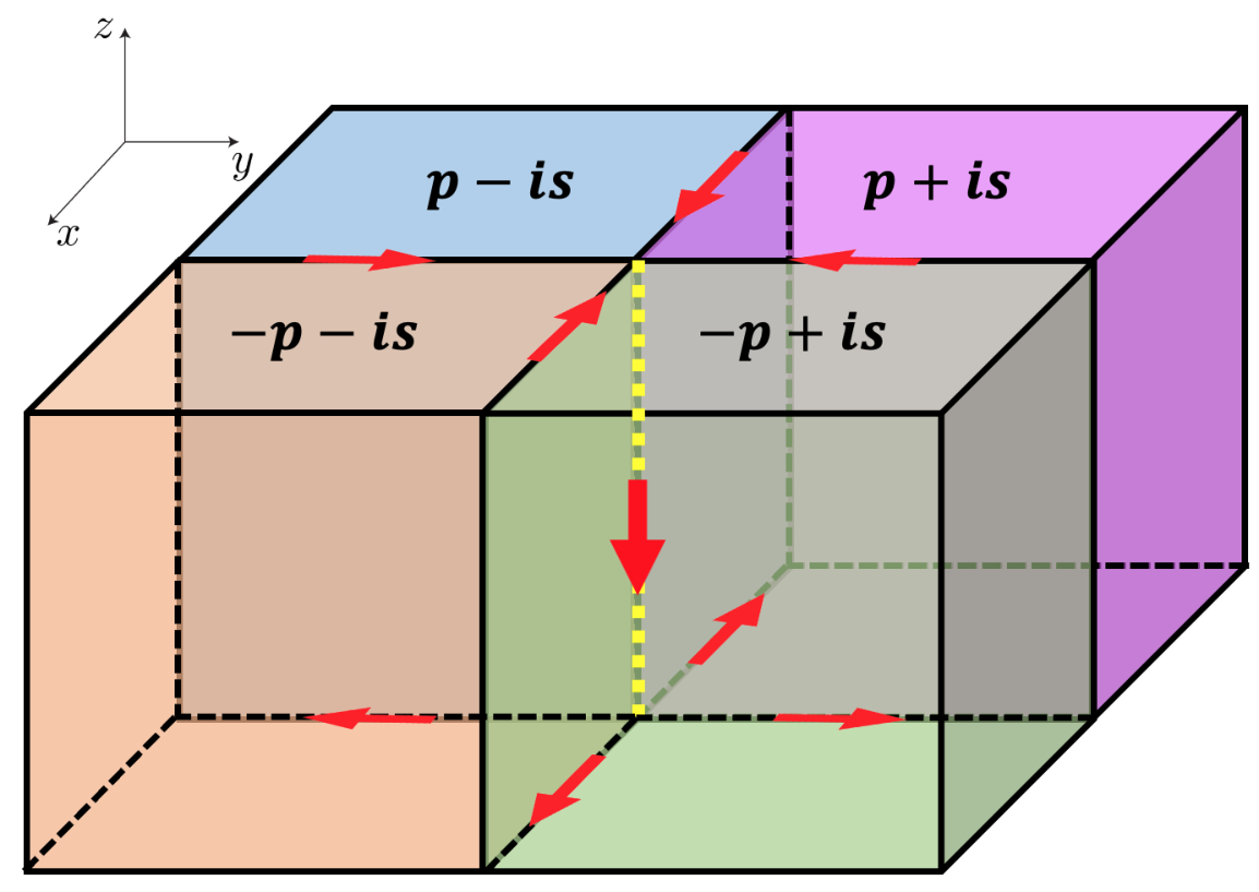
Figure 2: Electric currents on the surfaces of the superconducting bulk and along the vortex line, when a vortex line of Θax\Theta_{\text{ax}} is present. The red arrows denote the directions of the electric currents, and the yellow dashed line represents the location of the vortex core.

To understand the physical meaning of Eq. (85), we consider a vortex line of Θax\Theta_{\text{ax}} along zz-direction as shown in Fig. 2, where the x​yxy-coordinates of the vortex core are assumed to be x=y=0x=y=0, as represented by the yellow dashed line in Fig. 2. Fig. 2 represents a vortex line since the axion angles are different in p+i​sp+is, p−i​sp-is, −p+i​s-p+is, −p−i​s-p-is bulks, and in fact, Θax\Theta_{\text{ax}} winds by 2​π2\pi when these four bulks are successively traversed.

In addition, the surface of the superconducting bulk is the place where a sudden jump of ϕ\phi occurs, since the vacuum can be viewed as having very large electric potential such that all electrons are depleted. Hence, both ∇Θax\nabla\Theta_{\text{ax}} and ∇ϕ\nabla\phi are nonzero at the upper surface of the superconducting bulk. By virtue of j→(2)\vec{j}^{(2)} in Eq. (86), this leads to surface currents flowing to the vortex line as shown by the four red arrows on the upper surface in Fig. 2. The total inflowing current into the vortex line can be obtained by performing a line integral of j→(2)\vec{j}^{(2)} over a loop surrounding the vortex core on the upper surface, which gives

N˙=α​c12​π​∂z(ϕ+ℏ​∂tΦe),\dot{N}=\frac{\alpha c}{12\pi}\partial_{z}(\phi+\frac{\hbar\partial_{t}\Phi}{e}), (89)

where N˙\dot{N} represents the particle number injected into the vortex line per unit time.

Charge conservation is recovered j→(3)\vec{j}^{(3)} in Eq. (86). Notice that ∇×∇Θ\nabla\times\nabla\Theta is proportional to δ⁡(x)​δ​(y)\delta(x)\delta(y), hence it only has non-vanishing effects on the vortex line. Since ∇×∇Θ\nabla\times\nabla\Theta is parallel to the zz-direction, an integration ∫d​x​𝑑y​j→(3)\int dxdy\vec{j}^{(3)} gives the total current running along the vortex line. Performing the integral, we obtain

∫d​x​𝑑y​j→(3)\displaystyle\int dxdy\vec{j}^{(3)} =−α​c12​π​(ϕ+ℏ​∂tΦe)​z^.\displaystyle=-\frac{\alpha c}{12\pi}(\phi+\frac{\hbar\partial_{t}\Phi}{e})\hat{z}. (90)

The divergence of Eq. (90) gives the rate of change of particle number N˙\dot{N} as

N˙=∇⋅(∫dxdyj→(3))=−α​c12​π∂z(ϕ+ℏ​∂tΦe),\displaystyle\dot{N}=\nabla\cdot\big(\int dxdy\vec{j}^{(3)}\big)=-\frac{\alpha c}{12\pi}\partial_{z}(\phi+\frac{\hbar\partial_{t}\Phi}{e}), (91)

which exactly cancels with Eq. (89), ensuring the condition of charge conservation. Notice that N˙\dot{N} in Eq. (91) is nonzero only close to the upper surface. This is physically correct: The downward flowing current along the vortex line quickly increases as we go down the vortex line from the surface, since there are inflowing currents due to Eq. (89); on the other hand, deep in the bulk, the current reaches a steady flow along the vortex line, giving rise to a divergence free condition N˙=0\dot{N}=0.

VI.2 Witten effect

The second term in the density response (Eq. (84)) indicates a Witten effect in this system. Assuming a magnetic monopole at the origin of the bulk, we have ∇⋅B→∝δ(3)​(r→)\nabla\cdot\vec{B}\propto\delta^{(3)}(\vec{r}). An adiabatic change of a homogenous Θax\Theta_{\text{ax}} by Δ​Θax\Delta\Theta_{\text{ax}} leads to an accumulation of particles Δ​Q\Delta Q at the origin, which can be derived as

ΔQ=∫d3xdt∂tρ=∫d3xdt∂tΘax∇⋅B→∝ΔΘax.\Delta Q=\int d^{3}xdt\,\partial_{t}\rho=\int d^{3}xdt\,\partial_{t}\Theta_{\text{ax}}\,\nabla\cdot\vec{B}\propto\Delta\Theta_{\text{ax}}. (92)

VII Conclusion

In conclusion, we have studied the coupling between the axion field and the electromagnetic field in p+i​sp+is superconductors. We find that the axion electrodynamics in p+i​sp+is superconductors exhibits a nonrelativistic form, which is different from the superconducting Dirac or Weyl systems. As applications of the derived nonrelativistic axion action, the vortex lines of the axion angle and Witten effect are discussed. Our work reveals the crucial differences for axion electrodynamics between the p+i​sp+is superconductors and the superconducting Dirac/Weyl systems.

Acknowledgments CX is supported by Strategic Priority Research Program of CAS (No. XDB28000000) and The Office of Naval Research under Grant No. N00014-18-1-2722. WY is supported by the postdoctoral fellowship at Stewart Blusson Quantum Matter Institute, University of British Columbia.

Appendix A Real space calculation of transverse supercurrent

In this appendix, we perform a real space calculation of the transverse supercurrent induced by static electric field and spatial inhomogeneity of Δs\Delta_{s}. The corresponding term in the axion action SaxS_{\text{ax}} can then be determined from the relation ji=−c​δ​Sa​xδ​Aij_{i}=-c\frac{\delta S_{ax}}{\delta A_{i}} (i=1,2,3i=1,2,3) where cc is the light velocity. In addition to the orbital supercurrent discussed in this section, there is also bound current originating from the spin magnetic moment, as discussed in detail in Sec. V.

Recall that the expectation value of the current operator is given by Eq. (16), in which the Green’s function G^\hat{G} can be expressed as Eq. (18), where H2H^{2} is given by Eq. (19) and Eq. (20). Straightforward calculations show that

T^ρ​T^ρ\displaystyle\hat{T}^{\rho}\hat{T}^{\rho} =\displaystyle= [−ℏ22​m​∇2−μ⁡(r→)]2+Δp2kf2​(−∇2)+[Δs​(r→)]2,\displaystyle[-\frac{\hbar^{2}}{2m}\nabla^{2}-\mu(\vec{r})]^{2}+\frac{\Delta_{p}^{2}}{k_{f}^{2}}(-\nabla^{2})+[\Delta_{s}(\vec{r})]^{2},
[T^0,T^i]\displaystyle\text{$[$}\hat{T}^{0},\hat{T}^{i}\text{$]$} =\displaystyle= −iΔpkf∂iμ,\displaystyle-i\frac{\Delta_{p}}{k_{f}}\partial_{i}\mu,
[T^0,T^4]\displaystyle\text{$[$}\hat{T}^{0},\hat{T}^{4}\text{$]$} =\displaystyle= −ℏ22​m(∇2Δs+2∇Δs⋅∇),\displaystyle-\frac{\hbar^{2}}{2m}(\nabla^{2}\Delta_{s}+2\nabla\Delta_{s}\cdot\nabla),
[T^i,T^4]\displaystyle\text{$[$}\hat{T}^{i},\hat{T}^{4}\text{$]$} =\displaystyle= −iΔpkf∂iΔs,\displaystyle-i\frac{\Delta_{p}}{k_{f}}\partial_{i}\Delta_{s}, (93)

in which μ⁡(r→)=ϵF+e​ϕ​(r→)\mu(\vec{r})=\epsilon_{F}+e\phi(\vec{r}), where ϕ⁡(r→)\phi(\vec{r}) is the electric potential.

The n=0n=0 term in Eq. (21) vanishes: The odd-in-∂τ\partial_{\tau} term vanishes after Matsubara frequency summation; and the other terms contain a trace of a single γ\gamma-matrix, hence are also zero.

The n=1n=1 term also vanishes. Removing the odd-in-∂τ\partial_{\tau} term, the n=1n=1 term contains one ΔH\Delta_{H} and one HH under the trace operation. However, ΔH\Delta_{H} and HH are products of two and one γ\gamma-matrices, respectively. Hence the result vanishes since the trace of a product of three γ\gamma-matrices is zero.

Finally we consider the n=2n=2 term

⟨j^i(2)​(x→)⟩=\displaystyle\left<\hat{j}_{i}^{(2)}(\vec{x})\right>=
−Tr​[j^i​(x→)​1−∂τ2+H02​Q​1−∂τ2+H02​Q​1−∂τ2+H02​H].\displaystyle-\text{Tr}\big[\hat{j}_{i}(\vec{x})\frac{1}{-\partial_{\tau}^{2}+H_{0}^{2}}Q\frac{1}{-\partial_{\tau}^{2}+H_{0}^{2}}Q\frac{1}{-\partial_{\tau}^{2}+H_{0}^{2}}H\big]. (94)

To lowest order in the gradient expansion Niemi1986, μ⁡(r→)\mu(\vec{r}) and Δs​(r→)\Delta_{s}(\vec{r}) can be taken as constants in H0H_{0} Niemi1986. The only way to have a nonzero trace is a multiplication of all the five γ\gamma-matrices. Since the electric current operator j^i​(x→)\hat{j}_{i}(\vec{x}) contains a −i∂i-i\partial_{i}, the HH term must contribute Δpkf(−i∂i)γi\frac{\Delta_{p}}{k_{f}}(-i\partial_{i})\gamma^{i} so that the trace is nonzero. Therefore, we obtain

⟨j^i(2)(x→)⟩=2(Δpkf)3Tr[j^i(x→)1−∂τ2+H02∂jμ1−∂τ2+H02∂kΔs\displaystyle\left<\hat{j}_{i}^{(2)}(\vec{x})\right>=2(\frac{\Delta_{p}}{k_{f}})^{3}\text{Tr}\big[\hat{j}_{i}(\vec{x})\frac{1}{-\partial_{\tau}^{2}+H_{0}^{2}}\partial_{j}\mu\frac{1}{-\partial_{\tau}^{2}+H_{0}^{2}}\partial_{k}\Delta_{s}
×1−∂τ2+H02(−i∂i)]tr(γ0γjγkγ4γi).\displaystyle\times\frac{1}{-\partial_{\tau}^{2}+H_{0}^{2}}(-i\partial_{i})\big]\text{tr}(\gamma^{0}\gamma^{j}\gamma^{k}\gamma^{4}\gamma^{i}). (95)

in which the trace of the product of five γ\gamma-matrices can be easily evaluated using

tr​(γ0​γi​γj​γk​γ4)=−4​ϵi​j​k.\displaystyle\text{tr}(\gamma^{0}\gamma^{i}\gamma^{j}\gamma^{k}\gamma^{4})=-4\epsilon_{ijk}. (96)

Using Eq. (15), ⟨j^i(2)​(x→)⟩\left<\hat{j}_{i}^{(2)}(\vec{x})\right> can be evaluated as

⟨j^i(2)(x→)⟩=−ϵi​j​k2​e​ℏm(Δpkf)3∫dy→dz→\displaystyle\left<\hat{j}_{i}^{(2)}(\vec{x})\right>=-\epsilon_{ijk}\frac{2e\hbar}{m}(\frac{\Delta_{p}}{k_{f}})^{3}\int d\vec{y}d\vec{z}
{⟨x→|(−i∂i)1−∂τ2+H02|y→⟩∂jμ(y→)⟨y→|(−i∂i)1−∂τ2+H02|z→⟩\displaystyle\big\{\langle\vec{x}|(-i\partial_{i})\frac{1}{-\partial_{\tau}^{2}+H_{0}^{2}}|\vec{y}\rangle\partial_{j}\mu(\vec{y})\langle\vec{y}|(-i\partial_{i})\frac{1}{-\partial_{\tau}^{2}+H_{0}^{2}}|\vec{z}\rangle
×∂kΔs(z→)⟨z→|1−∂τ2+H02(−i∂i)|x→⟩\displaystyle\penalty\ \penalty\ \penalty\ \penalty\ \penalty\ \penalty\ \times\partial_{k}\Delta_{s}(\vec{z})\langle\vec{z}|\frac{1}{-\partial_{\tau}^{2}+H_{0}^{2}}(-i\partial_{i})|\vec{x}\rangle
+⟨x→|1−∂τ2+H02|y→⟩∂jμ(y→)⟨y→|1−∂τ2+H02|z→⟩∂kΔs(z→)\displaystyle+\langle\vec{x}|\frac{1}{-\partial_{\tau}^{2}+H_{0}^{2}}|\vec{y}\rangle\partial_{j}\mu(\vec{y})\langle\vec{y}|\frac{1}{-\partial_{\tau}^{2}+H_{0}^{2}}|\vec{z}\rangle\partial_{k}\Delta_{s}(\vec{z})
×⟨z→|1−∂τ2+H02(−i∂i)2|x→⟩}.\displaystyle\penalty\ \penalty\ \penalty\ \penalty\ \penalty\ \penalty\ \times\langle\vec{z}|\frac{1}{-\partial_{\tau}^{2}+H_{0}^{2}}(-i\partial_{i})^{2}|\vec{x}\rangle\big\}. (97)

In momentum space, Eq. (97) becomes

⟨j^i(2)​(x→)⟩=−ϵi​j​k​2​e​ℏm​(Δpkf)3\displaystyle\left<\hat{j}_{i}^{(2)}(\vec{x})\right>=-\epsilon_{ijk}\frac{2e\hbar}{m}(\frac{\Delta_{p}}{k_{f}})^{3}
×1β​∑ωn∫d​y→​𝑑z→​∂jμ⁡(y)​∂kΔs​(z)​[Πα=13​∫d​k→α(2​π)3]\displaystyle\times\frac{1}{\beta}\sum_{\omega_{n}}\int d\vec{y}d\vec{z}\partial_{j}\mu(y)\partial_{k}\Delta_{s}(z)\big[\Pi_{\alpha=1}^{3}\int\frac{d\vec{k}_{\alpha}}{(2\pi)^{3}}\big]
×(k1​i​k3​i+k3​i2)​[Πα=13​1ωn2+[H0​(k→α)]2​ei​kα⋅(r→α−r→α+1)],\displaystyle\times(k_{1i}k_{3i}+k_{3i}^{2})\big[\Pi_{\alpha=1}^{3}\frac{1}{\omega_{n}^{2}+[H_{0}(\vec{k}_{\alpha})]^{2}}e^{ik_{\alpha}\cdot(\vec{r}_{\alpha}-\vec{r}_{\alpha+1})}\big], (98)

in which β\beta is the inverse temperature; ωn=(2​n+1)​π/β\omega_{n}=(2n+1)\pi/\beta is the fermionic Matsubara frequency; r→1,2,3=x→,y→,z→\vec{r}_{1,2,3}=\vec{x},\vec{y},\vec{z}; and r→4=r→1\vec{r}_{4}=\vec{r}_{1}.

To lowest order in the gradient expansion, we can set y→=z→\vec{y}=\vec{z} in ∂jμ⁡(y→)​∂kΔs​(z→)\partial_{j}\mu(\vec{y})\partial_{k}\Delta_{s}(\vec{z}) within Eq. (98), then integrating over z→\vec{z} gives a momentum delta function δ(3)​(k→2−k→3)\delta^{(3)}(\vec{k}_{2}-\vec{k}_{3}). Furthermore, if the higher order terms in the gradient expansion are neglected, then y→\vec{y} can be set as x→\vec{x} in ∂jμ⁡(y→)​∂kΔs​(y→)\partial_{j}\mu(\vec{y})\partial_{k}\Delta_{s}(\vec{y}), and the integration over y→\vec{y} gives δ(3)​(k→1−k→2)\delta^{(3)}(\vec{k}_{1}-\vec{k}_{2}). As a result, we obtain ji​(x→)=∑n=02⟨j^i(n)​(x→)⟩j_{i}(\vec{x})=\sum_{n=0}^{2}\left<\hat{j}_{i}^{(n)}(\vec{x})\right> as

ji​(x→)=e2​D​(Δs,Δp)​ϵi​j​k​∂jϕ⁡(x→)​∂kΔs​(x→),\displaystyle j_{i}(\vec{x})=e^{2}D(\Delta_{s},\Delta_{p})\epsilon_{ijk}\partial_{j}\phi(\vec{x})\partial_{k}\Delta_{s}(\vec{x}), (99)

in which ∂jμ=−e∂jϕ\partial_{j}\mu=-e\partial_{j}\phi is used, and the coefficient DD is

D(Δs,Δp)=4​ℏm(Δpkf)3×\displaystyle D(\Delta_{s},\Delta_{p})=\frac{4\hbar}{m}(\frac{\Delta_{p}}{k_{f}})^{3}\times
1β​∫d3​k(2​π)3​k2/3[ωn2+ξ2​(k→)+(Δpkf)2​k2+Δs2]3,\displaystyle\frac{1}{\beta}\int\frac{d^{3}k}{(2\pi)^{3}}\frac{k^{2}/3}{[\omega_{n}^{2}+\xi^{2}(\vec{k})+(\frac{\Delta_{p}}{k_{f}})^{2}k^{2}+\Delta_{s}^{2}]^{3}}, (100)

where the replacement ki2→k2/3k_{i}^{2}\rightarrow k^{2}/3 is used which holds under integration. For simplicity, we consider zero temperature such that 1β∑n\frac{1}{\beta}\sum_{n} can be replaced by ∫d​ω2​π\int\frac{d\omega}{2\pi}. In the weak pairing limit Δs/ϵF,Δp/ϵF≪1\Delta_{s}/\epsilon_{F},\Delta_{p}/\epsilon_{F}\ll 1, kk can be simply taken as kfk_{f} in (Δpkf​k)2(\frac{\Delta_{p}}{k_{f}}k)^{2} in the denominator, and ∫𝑑k=∫𝑑ξ/(ℏ​vf)\int dk=\int d\xi/(\hbar v_{f}) where vf=ℏ​kf/mv_{f}=\hbar k_{f}/m is the Fermi velocity. Eq. (100) can then be evaluated, yielding

D⁡(Δs,Δp)=16​π2​ℏ​Δp3(Δp2+Δs2)2,\displaystyle D(\Delta_{s},\Delta_{p})=\frac{1}{6\pi^{2}\hbar}\frac{\Delta_{p}^{3}}{(\Delta_{p}^{2}+\Delta_{s}^{2})^{2}}, (101)

which is Eq. (24).

Appendix B Symmetry allowed non-axion terms

In this appendix we examine all the symmetry allowed terms which contain one Δλ\Delta_{\lambda} (λ=s,p\lambda=s,p), two AμA^{\mu}’s (μ=t,x,y,z\mu=t,x,y,z), and two spacetime derivatives. Up to an overall factor F⁡(Δs2,Δs/Δp)​ΔλF(\Delta_{s}^{2},\Delta_{s}/\Delta_{p})\Delta_{\lambda} (where FF is a function which can be determined by calculating the corresponding diagram), the terms invariant under 3D rotations and 𝒫​𝒯\mathcal{PT}-operation are

∂tA→′⋅∂tA→′​δ​Δλ\displaystyle\partial_{t}\vec{A}^{\prime}\cdot\partial_{t}\vec{A}^{\prime}\penalty\ \delta\Delta_{\lambda}
∂t2A→′⋅A→′​δ​Δλ\displaystyle\partial_{t}^{2}\vec{A}^{\prime}\cdot\vec{A}^{\prime}\penalty\ \delta\Delta_{\lambda}
∂tϕ′​∂tϕ′​δ​Δλ\displaystyle\partial_{t}\phi^{\prime}\partial_{t}\phi^{\prime}\penalty\ \delta\Delta_{\lambda}
∂t2ϕ′​ϕ′​δ​Δλ\displaystyle\partial_{t}^{2}\phi^{\prime}\penalty\ \phi^{\prime}\penalty\ \delta\Delta_{\lambda} (102)
(∇⋅A→′)​(∇⋅A→′)​δ​Δλ\displaystyle(\nabla\cdot\vec{A}^{\prime})(\nabla\cdot\vec{A}^{\prime})\penalty\ \delta\Delta_{\lambda}
∇2A→′⋅A→′​δ​Δλ\displaystyle\nabla^{2}\vec{A}^{\prime}\cdot\vec{A}^{\prime}\penalty\ \delta\Delta_{\lambda}
∇ϕ′⋅∇ϕ′δΔλ\displaystyle\nabla\phi^{\prime}\cdot\nabla\phi^{\prime}\penalty\ \delta\Delta_{\lambda}
∇2ϕ′​ϕ′​δ​Δλ\displaystyle\nabla^{2}\phi^{\prime}\penalty\ \phi^{\prime}\penalty\ \delta\Delta_{\lambda} (103)
∂tA→′⋅(∇×A→′)​δ​Δλ\displaystyle\partial_{t}\vec{A}^{\prime}\cdot(\nabla\times\vec{A}^{\prime})\penalty\ \delta\Delta_{\lambda}
A→′⋅(∇×∂tA→′)​δ​Δλ\displaystyle\vec{A}^{\prime}\cdot(\nabla\times\partial_{t}\vec{A}^{\prime})\penalty\ \delta\Delta_{\lambda} (104)
(∇⋅A→′)​∂tϕ′​δ​Δλ\displaystyle(\nabla\cdot\vec{A}^{\prime})\partial_{t}\phi^{\prime}\penalty\ \delta\Delta_{\lambda} (105)
(∇×A→′)⋅(∇ϕ′)​δ​Δλ,\displaystyle(\nabla\times\vec{A}^{\prime})\cdot(\nabla\phi^{\prime})\penalty\ \delta\Delta_{\lambda}\,, (106)

in which λ=s,p\lambda=s,p. The terms in Eq. (104) vanish as discussed in Sec. IV.1, and Eq. (106) is the axion term which has been calculated and discussed in the main text.

Here we make a comment on the order of the coefficients of the non-axion terms. In superconductors, the leading term in the action for the phase mode is

∫d4x[Nf(ℏ∂tΦ+eϕ)2−ns2​m(ℏ∇Φ+e​A→c)2],\displaystyle\int d^{4}x\big[N_{f}(\hbar\partial_{t}\Phi+e\phi)^{2}-\frac{n_{s}}{2m}(\hbar\nabla\Phi+\frac{e\vec{A}}{c})^{2}\big], (107)

in which nsn_{s} is the superfluid density. Notice that in the long wavelength limit, additional spacetime gradient terms are suppressed by factor of (q​ξc)n∼(ℏ​vf​q/Δ)n(q\xi_{c})^{n}\sim(\hbar v_{f}q/\Delta)^{n} Altland2010, where ξc\xi_{c} is the coherence length, and qq can be either |q→||\vec{q}| or |Ω|/vf|\Omega|/v_{f}. For simplicity, consider the term ∂tA→⋅∇×A→\partial_{t}\vec{A}\cdot\nabla\times\vec{A} (although this term vanishes as discussed in Eq. (104), it works as an illustration for the other non-axion terms, regarding the order of the coefficients). The coefficient CC of this term should be on order of ∼1Δ​(vfΔ)​ns2​m\sim\frac{1}{\Delta}(\frac{v_{f}}{\Delta})\frac{n_{s}}{2m}. Using ns∼kf3n_{s}\sim k_{f}^{3}, it is straightforward to obtain C∼(ϵf/Δ)2C\sim(\epsilon_{f}/\Delta)^{2}. On the other hand, recall that the coefficients of the axion terms are of O⁡[(Δ/ϵf)0]O[(\Delta/\epsilon_{f})^{0}]. Therefore, generically, the non-axion terms can be much larger, i.e., enhanced by a factor of (ϵf/Δ)2(\epsilon_{f}/\Delta)^{2} compared with the axion terms. However, we note that none of the non-axion terms can contribute to the effects like transverse supercurrent as discussed in Sec. A, and in fact, they do not exhibit magnetoelectric effects.

References

  • (1) A. J. Leggett, Rev. Mod. Phys. 47, 331 (1975).
  • (2) D. Vollhardt and P. Wölfle, The Superfluid Phases of Helium 3 (Taylor and Francis, London, 1990).
  • (3) G. E. Volovik, The Universe in a Helium Droplet (Oxford University Press, New York, 2003).
  • (4) A. P. Mackenzie and Y. Maeno, Rev. Mod. Phys. 75, 657 (2003).
  • (5) A. J. Leggett, Quantum Liquids (Oxford University, New York, 2006).
  • (6) M. Z. Hasan and C. L. Kane, Rev. Mod. Phys. 82, 3045 (2010).
  • (7) X.-L. Qi and S.-C. Zhang, Rev. Mod. Phys. 83, 1057 (2011).
  • (8) Y. Ando and L. Fu, Annu. Rev. Condens. Matter Phys. 6, 361 (2015).
  • (9) M. Sato and S. Fujimoto, J. Phys. Soc. Jpn. 85, 072001 (2016).
  • (10) C.-K. Chiu, J. C. Y. Teo, A. P. Schnyder, and S. Ryu, Rev. Mod. Phys. 88, 035005 (2016).
  • (11) M. Sato and Y. Ando, Rep. Prog. Phys. 80, 076501 (2017).
  • (12) G. Volovik, Phys. Lett. A 128, 277 (1988).
  • (13) G. Volovik and V. Yakovenko, J. Phys. Condens. Matter 1, 5263 (1989).
  • (14) D. A. Ivanov, Phys. Rev. Lett. 86, 268 (2001).
  • (15) N. B. Kopnin and M. M. Salomaa, Phys. Rev. B 44, 9667 (1991).
  • (16) M. Stone and S.-B. Chung, Phys. Rev. B 73, 014505 (2006).
  • (17) S. Tewari, S. Das Sarma, C. Nayak, C. Zhang, and P. Zoller, Phys. Rev. Lett. 98, 010506 (2007).
  • (18) C. Zhang, S. Tewari, R. M. Lutchyn, and S. Das Sarma, Phys. Rev. Lett. 101, 160401 (2008).
  • (19) L. Fu and C. L. Kane, Phys. Rev. Lett. 100, 096407 (2008).
  • (20) M. Cheng, K. Sun, V. Galitski, and S. Das Sarma, Phys. Rev. B 81, 024504 (2010).
  • (21) X.-L. Qi, T. L. Hughes, S. Raghu, and S.-C. Zhang, Phys. Rev. Lett. 102, 187001 (2009).
  • (22) Y. Wang and A. Chubukov, Phys. Rev. B 90, 035149 (2014).
  • (23) Y. Wang and L. Fu, Phys. Rev. Lett. 119, 187003 (2017).
  • (24) W. Yang, C. Xu, and C. Wu, Phys. Rev. Research 2, 042047(R) (2020).
  • (25) C. Xu, W. Yang, and C. Wu, arXiv:2010.05362 (2020).
  • (26) W.-C. Lee, S.-C. Zhang, and C. Wu, Phys. Rev. Lett. 102, 217002 (2009).
  • (27) Y. Li, D. Wang, C. Wu, New Journal of Physics 15 (8), 085002 (2013).
  • (28) R. Thomale, C. Platt, W. Hanke, and B. A. Bernevig, Phys. Rev. Lett. 106, 187003 (2011).
  • (29) C. Platt, R. Thomale, C. Honerkamp, S.-C. Zhang, and W. Hanke, Phys. Rev. B 85, 180502 (2012).
  • (30) M. Khodas and A. V. Chubukov, Phys. Rev. Lett. 108, 247003 (2012).
  • (31) R. M. Fernandes and A. J. Millis, Phys. Rev. Lett. 111, 127001 (2013).
  • (32) A. Hinojosa, R. M. Fernandes, and A. V. Chubukov, Phys. Rev. Lett. 113, 167001 (2014).
  • (33) V. Stanev and Z. Tešanovíc, Phys. Rev. B 81, 134522 (2010).
  • (34) S.-Z. Lin and X. Hu, Phys. Rev. Lett. 108, 177005 (2012).
  • (35) M. Marciani, L. Fanfarillo, C. Castellani, and L. Benfatto, Phys. Rev. B 88, 214508 (2013).
  • (36) S. Maiti and A. V. Chubukov, Phys. Rev. B 87, 144511 (2013).
  • (37) F. Ahn, I. Eremin, J. Knolle, V. B. Zabolotnyy, S. V. Borisenko, B. Büchner, and A. V. Chubukov, Phys. Rev. B 89, 144513 (2014).
  • (38) J. Garaud and E. Babaev, Phys. Rev. Lett. 112, 017003 (2014).
  • (39) S. Maiti, M. Sigrist, and A. Chubukov, Phys. Rev. B 91, 161102 (2015).
  • (40) R. B. Laughlin, Phys. Rev. Lett. 80, 5188 (1998).
  • (41) T. Senthil, J. B. Marston, and M. P. A. Fisher, Phys. Rev. B 60, 4245 (1999).
  • (42) B. Horovitz and A. Golub, Phys. Rev. B 68, 214503 (2003).
  • (43) Y. Jiang, D.-X. Yao, E. W. Carlson, H.-D. Chen, and J. Hu, Phys. Rev. B 77, 235420 (2008).
  • (44) M. Sato, Y. Takahashi, and S. Fujimoto, Phys. Rev. B 82, 134521 (2010).
  • (45) A. M. Black-Schaffer, Phys. Rev. Lett. 109, 197001 (2012).
  • (46) R. Nandkishore, L. S. Levitov, and A. V. Chubukov, Nat. Phys. 8, 158 (2012).
  • (47) W.-S. Wang, Y.-Y. Xiang, Q.-H. Wang, F. Wang, F. Yang, and D.-H. Lee, Phys. Rev. B 85, 035414 (2012).
  • (48) M. L. Kiesel, C. Platt, W. Hanke, and R. Thomale, Phys. Rev. Lett. 111, 097001 (2013).
  • (49) F. Liu, C.-C. Liu, K. Wu, F. Yang, and Y. Yao, Phys. Rev. Lett. 111, 066804 (2013).
  • (50) A. M. Black-Schaffer and C. Honerkamp, J. Phys.: Condens. Matter. 26 423201 (2014.)
  • (51) C. Wu and J. Hirsch, Phys. Rev. B 81, 020508 (2010).
  • (52) A. J. Niemi and G. W. Semenoff, Phys. Rep. 135, 99 (1986).
  • (53) S. Ryu, J. E. Moore, and A. W. W. Ludwig, Phys. Rev. B 85, 045104 (2012).
  • (54) X.-L. Qi, E. Witten, and S.-C. Zhang, Phys. Rev. B 87, 134519 (2013).
  • (55) Z. Wang, X. L. Qi, and S. C. Zhang, Phys. Rev. B 84, 014527 (2011).
  • (56) N. Read and D. Green, Phys. Rev. B 61, 10267 (2000).
  • (57) M. Stone, Phys. Rev. B 85, 184503 (2012).
  • (58) B. Roy, Phys. Rev. B 101, 220506 (2020).
  • (59) T. Shang, M. Smidman, S. K. Ghosh, C. Baines, L. J. Chang, D. J. Gawryluk, J. A. T. Barker, R. P. Singh, D. Mck. Paul, G. Balakrishnan, E. Pomjakushina, M. Shi, M. Medarde, A. D. Hillier, H. Q. Yuan, J. Quintanilla, J. Mesot, and T. Shiroka, Phys. Rev. Lett. 121, 257002 (2018).
  • (60) S. Sundar, S Salem-Sugui Jr , M K Chattopadhyay, S B Roy, L S Sharath Chandra, L F Cohen, and L Ghivelder, Supercond. Sci. Technol. 32 055003 (2019).
  • (61) R. D. Peccei and H. R. Quinn, Phys. Rev. Lett. 38, 1440 (1977).
  • (62) S. Weinberg, Phys. Rev. Lett. 40, 223 (1978).
  • (63) F. Wilczek, Phys. Rev. Lett. 40, 279 (1978).
  • (64) R. Li, J. Wang, X.-L. Qi, and S.-C. Zhang, Nat. Phys. 6, 284 (2010).
  • (65) P. Goswami, B. Roy, Phys. Rev. B 90, 041301(R) (2014).
  • (66) K. Shiozaki and S. Fujimoto, Phys. Rev. B 89, 054506 (2014).
  • (67) M. Stone, P. L. S. Lopes, Phys. Rev. B 93, 174501 (2016).
  • (68) A. Atland and B. Simons, Condensed Matter Field Theory (Cambridge University Press, New York, 2010).