跳到论文正文
W Papers独立论文阅读器 arXiv:2009.12545 论文正文 计算阅读时间 · 0%
引用这篇论文根据当前论文元数据生成,正式投稿前建议核对。


License: arXiv.org perpetual non-exclusive license
arXiv:2009.12545v1 [math.OC] 26 Sep 2020

A Continuous-Time Nesterov Accelerated Gradient Method for Centralized and Distributed Online Convex Optimization

Chao Sun    Guoqiang Hu Thanks: This work was supported by Singapore Ministry of Education Academic Research Fund Tier 1 RG180/17(2017-T1-002-158). C. Sun and G. Hu are with the School of Electrical and Electronic Engineering, Nanyang Technological University, Singapore 639798 (email: csun002@e.ntu.edu.sg, gqhu@ntu.edu.sg).
Abstract

This paper studies the online convex optimization problem by using an Online Continuous-Time Nesterov Accelerated Gradient method (OCT-NAG). We show that the continuous-time dynamics generated by the online version of the Bregman Lagrangian achieves a constant static regret cσ\frac{c}{\sigma} independent of TT, provided that some boundedness assumptions on the objective functions and optimal solutions hold. To the best of the authors’ knowledge, this is the lowest static regret in the literature (lower than O​(log​(T))O(\text{log}(T))). We further show that under the same assumptions, the dynamic regret of the algorithm is O⁡(T)O(T), which is comparable with the existing methods. Simulation results validate the effectiveness and efficiency of the method. Furthermore, the simulation shows that the algorithm performs well in terms of the dynamic regret for some specific scaling conditions. In addition, we consider the application of the proposed online optimization method in distributed online optimization problems, and show that the proposed algorithm achieves an O⁡(T)O(\sqrt{T}) static regret, which is comparable with the existing distributed online optimization methods. Different from these methods, the proposed method requires neither the gradient boundedness assumption nor the compact constraint set assumption, which allows different objective functions and different optimization problems with those in the literature. A comparable dynamic regret is obtained. Simulation results show the effectiveness and efficiency of the distributed algorithm.

Index Terms: 
Online optimization; Nesterov Accelerated Gradient; Continuous-time dynamics; Regret analysis; Distributed online optimization

I Introduction

Optimization plays an important role in many areas such as robotics, machine learning, finance, power electronics, and military, etc. Till now, numerous optimization methods have been developed with applications to different scenarios and for different algorithm requirements. Some popular methods include first-order gradient based methods (Gradient Descent, Projected Subgradient, Mirror Descent, Proximal Gradient, Alternating Direction Method of Multiplier (ADMM), etc), second-order Hessian based methods (Newton’s method, Gauss-Newton, etc), Conjugate Gradient Method and stochastic optimization methods (Stochastic Gradient Descent, etc), to name a few [1, 2].

Convergence rate is one of the most important criteria to evaluate the performance of an optimization algorithm. Among all first-order gradient based methods, Nesterov Accelerated Gradient method has the optimal convergence rate according to first-order oracle complexity [3, 4]. The acceleration feature makes the method become one of the most popular optimization methods and has a wide range of applications in many areas such as deep learning. Recently, there are also some further studies on Nesterov Accelerated Gradient methods in multi-agent systems. For example, [5] studied the applications of the algorithm in distributed optimization problems and [6] applied the algorithm to distributively seek a Nash equilibrium of a noncooperative game.

The Nesterov Accelerated Gradient method is being studied and explained from a continuous-time dynamical system perspective [7, 8]. In [7], a second-order ordinary differential equation (ODE) was derived which has an approximate equivalence to the discrete-time Nesterov Accelerated Gradient method in terms of the convergence rate. Surprisingly, the continuous-time ODE generates a family of schemes with higher order convergence rates O⁡(1kr),r≥2O(\frac{1}{k^{r}}),r\geq 2 than O⁡(1k2)O(\frac{1}{k^{2}}) in [3]. In [8], a Bregman Lagrangian function was defined. Taking the Euler-Lagrange curve of the function generates a family of continuous-time ODEs, which are more general than the ODEs in [7]. It was proven that these ODEs can achieve an arbitrary polynomial-order convergence rate and an exponential convergence rate under different scaling conditions (similar to the step-size concept) for a convex function. These interesting findings make the continuous-time methods attract more and more attentions recently. For example, [9] explored the differential inclusion version of the algorithm by using nonsmooth analysis theory.

Online optimization was first defined in machine learning, which solves a class of optimization problems where the objective function is time-varying [10]. At each iteration kk, the decision maker makes a decision xkx_{k} according to the previous knowledge. After that, the decision maker receives its objective function fkf_{k} of iteration kk. In other words, the decision maker uses the previous information to help make a decision for the present optimization problem. For example, for an Online Gradient Descent method,

x(tk+1)=P𝒞(x(tk)−ηk∇ftk(x(tk))),\displaystyle x(t_{k+1})=P_{\mathcal{C}}(x(t_{k})-\eta_{k}\nabla f_{t_{k}}(x(t_{k}))), (1)

where x⁡(tk)x(t_{k}) is the decision variable at iteration kk, P𝒞P_{\mathcal{C}} is the projection onto the feasible set, ηk\eta_{k} is the step-size and ftk​(x​(tk))f_{t_{k}}(x(t_{k})) is the objective function at iteration kk. The information at iteration kk is used to generate a decision for iteration k+1k+1. The online optimization problem was also studied in a continuous-time sense. In [11], a continuous-time gradient-based method was proposed as follows:

x˙=−γ∇ft(x),\displaystyle\dot{x}=-\gamma\nabla f_{t}(x), (2)

where γ\gamma is a fixed gain. The present information ft​(x)f_{t}(x) is used to help generate the guidance (i.e., x˙\dot{x}) for the next moment. In addition, some distributed continuous-time online optimization algorithms were proposed in [12, 13].

The regret is usually used to evaluate the effectiveness of an algorithm. The static regret refers to the accumulated difference between the cost function computed according to the value of the algorithm variable and the cost function computed according to the best fixed point that minimizes the accumulated cost function [10], i.e., for a positive integer KK and T=K​hT=Kh with hh being the sampling period,

ℛd​s​(T)=∑tk=T0T(ftk​(x⁡(tk))−ftk​(x~​(T))),\displaystyle\mathcal{R}_{ds}(T)=\sum_{t_{k}=T_{0}}^{T}(f_{t_{k}}(x(t_{k}))-f_{t_{k}}(\tilde{x}(T))), (3)

where x~​(T)=argminx∈𝒞​∑k=0Kftk​(x)\tilde{x}(T)=\text{argmin}_{x\in\mathcal{C}}\sum_{k=0}^{K}f_{t_{k}}(x) is a comparator in an offline sense. The dynamic regret is an online comparator which can be defined as

ℛd​d​(T)=∑tk=T0T(ftk​(x⁡(tk))−ftk​(x∗​(tk))),\displaystyle\mathcal{R}_{dd}(T)=\sum_{t_{k}=T_{0}}^{T}(f_{t_{k}}(x(t_{k}))-f_{t_{k}}(x^{*}(t_{k}))), (4)

where x∗​(tk)x^{*}(t_{k}) is the optimal solution of the optimization problem at iteration kk. Similarly, a recent paper defines the regrets in a continuous-time perspective [14].

Some popular online optimization algorithms include Online Gradient Descent, Adaptive Gradient Method (AdaGrad), Online Mirror Descent, Online Newton Step, Follow-The-Approximate-Leader (FTAL), etc. Under the assumption that the gradients are bounded, it was shown that the static regret for Online Gradient Descent is O⁡(T)O(\sqrt{T}) [15] (under the gradient boundedness assumption, the bound is tight ), and the regret bound can be relaxed to O​(log​(T))O(\text{log}(T)) for strongly convex functions. Under the gradient boundedness assumption and the exp-concavity assumption on the convex cost functions (which is more general than strong convexity [16]), it was proven that the Online Newton Step and FTAL can achieve O​(log​(T))O(\text{log}(T)) static regrets. See Table I for the static regrets and conditions for these algorithms.

Distributed optimization aims to solve a class of network optimization problems with multiple agents where the objective function is the sum of all the agents’ local objective functions [17, 12, 18]. The agents collaborate with each other to solve the optimization problem by using only neighboring information in the communication topology. Distributed online optimization deals with time-varying cost functions, and is attracting more and more attentions in many areas such as decentralized tracking [19] and swarm robots [13]. In addition to the above-mentioned continuous-time algorithms [12, 13], there are some discrete-time algorithms developed for distributed online optimization problems. For example, a distributed dual averaging method was proposed in [20] and an O⁡(T)O(\sqrt{T}) static regret was proven. A Distributed Online Mirror Descent method was proposed in [19] and the algorithm achieves an O⁡(T⁡(1+VT))O(\sqrt{T(1+V_{T})}) dynamic regret, where VTV_{T} is a TT-related function. An online subgradient descent algorithm with proportional-integral disagreement feedback was proposed in [21]. O⁡(T)O(\sqrt{T}) and O​(log​(T))O(\text{log}(T)) regrets were proven under different assumptions. A saddle point algorithm was proposed in [22] with an O⁡(T)O(\sqrt{T}) static regret. In [23], Distributed Weighted Dual Averaging was proposed with an O⁡(T)O(\sqrt{T}) static regret.

Based on the above knowledge, this work aims to answer the following question: Whether the continuous-time Nesterov Accelerated Gradient method could be used to solve online optimization problems? Under what assumptions, what kind of static regrets and dynamic regrets could be guaranteed? What is the performance of the algorithm in distributed online optimization problems?

Motivated by [8], We analyze the static regret and the dynamic regret of the Euler-Lagrange ODE generated by the online version of the Bregman Lagrangian function. Then, we design a distributed algorithm for distributed online optimization problems and analyze its performance. The main contributions are listed as follows:

(1) We prove that under some scaling conditions and under some boundedness assumptions, the static regret of the OCT-NAG is cσ\frac{c}{\sigma} which is a constant independent of TT. This relaxes the static regrets in the literature. As a comparison, in addition to the O​(log​(T))O(\text{log}(T)) regrets for the algorithms in Table I, the most related work may be [24] where a (log​(T)−log​(log​(T))+O⁡(log​(log​(T))log​(T)))(\text{log}(T)-\text{log}(\text{log}(T))+O(\frac{\text{log}(\text{log}(T))}{\text{log}(T)})) regret was found for some quadratic functions with some additional assumptions on the cost functions. To the best of the authors’ knowledge, the proposed method achieves the lowest static regret bound in the literature.

(2) We prove that under the same scaling conditions, the dynamic regret of OCT-NAG is O⁡(T)O(T). This regret is comparable with the regrets of the existing methods in the literature. Most of the algorithms achieve similar dynamic regrets. For example, the Online Gradient Descent [15] achieves an O⁡(T)O(T) dynamic regret for fixed step-sizes. The Dynamic Mirror Descent in [25] achieves an O​(T​(1+VT))O(\sqrt{T}(1+V_{T})) dynamic regret. A restarted Online Gradient Descent method in [26] was proven to have a O⁡(T23​(VT+1)13)O(T^{\frac{2}{3}}(V_{T}+1)^{\frac{1}{3}}) dynamic regret. Moreover, we show in the simulation that for some specific scaling conditions (i.e., eαt+βt−β˙t​eβt=σ⁡(t+b0)e^{\alpha_{t}+\beta_{t}}-\dot{\beta}_{t}e^{\beta_{t}}=\sigma(t+b_{0})), the algorithm has a better performance in terms of the dynamic regrets than other compared algorithms.

(3) The proposed Distributed Online Continuous-Time Nesterov Accelerated Gradient method (DOCT-NAG) achieves a comparable static regret with the methods in the literature (O⁡(T)O(\sqrt{T})). The algorithm requires neither the gradient boundedness assumption nor the projection onto a compact set, which could be used to solve different optimization problems with the literature [20, 19, 21, 22, 23].

(4) The discrete-time Nesterov Accelerated Gradient methods have been studied from various perspectives for static optimization/game problems [5, 6], and there are also some literature on their applications to online optimization[27]. However, different from [5, 6, 27], we investigate the Online Continuous-Time Nesterov Accelerated Gradient method and obtain lower static regrets than [27]. In addition, most of the existing literature on online optimization are based on discrete-time algorithms. The continuous-time framework in this work allows for the possibility of solving optimization problems using well-established theories in ODE and control theory.

The rest of the paper is organized as follows: In Section II, notations and preliminary knowledge on graph theory and convex optimization is given. In Section III, the static regret and the dynamic regret of OCT-NAG are analyzed. In Section IV, the static regret and the dynamic regret of DOCT-NAG are given. In Section V, simulation results show the effectiveness and efficiency of the proposed algorithms. Finally, Section VI concludes the paper.

II Notations and Preliminaries

Notations: Letting 𝒞\mathcal{C} being a convex set, the notation argminx∈𝒞⁡f⁡(x)\mathop{\text{argmin}}\limits_{x\in\mathcal{C}}f(x) represents the decision variable value x∈𝒞x\in\mathcal{C} such that the function f⁡(x)f(x) takes its minimum. ‖⋅‖\left\|\cdot\right\| is the Euclidean norm and |⋅|\left|\cdot\right| is the absolute value. log(⋅)(\cdot) represents the natural logarithm. “00” represents a zero scalar or vector with a appropriate dimension. 1N1_{N} is an N×1N\times 1 column vector with all elements being 1.

Graph Theory: Let 𝒢={𝒱,ℰ}\mathcal{G}=\left\{\mathcal{V},\mathcal{E}\right\} denote an undirected graph, where 𝒱={1,…,N}\mathcal{V=}\left\{1,...,N\right\} is the vertex set and ℰ⊂𝒱×𝒱\mathcal{E\subset V\times V} is the edge set. 𝒩i={j∈𝒱∣(j,i)∈ℰ}\mathcal{N}_{i}=\left\{j\in\mathcal{V\mid}(j,i)\in\mathcal{E}\right\} denotes the set of neighbors of vertex ii. A path is referred by the sequence of its vertices. Path 𝒫\mathcal{P} between v0v_{0} and vmv_{m} is the sequence {v0,…,vm}\left\{v_{0},...,v_{m}\right\} where (vi−1,vi)∈ℰ(v_{i-1},v_{i})\in\mathcal{E} for i=1,…,mi=1,...,m and the vertices are distinct. The number mm is defined as the length of path 𝒫\mathcal{P}. Graph 𝒢\mathcal{G} is connected if for any two vertices, there is a path in 𝒢\mathcal{G}. A matrix A=[ai​j]∈ℝN×NA=\left[a_{ij}\right]\in\mathbb{R}^{N\times N} denotes the adjacency matrix of 𝒢\mathcal{G}, where ai​j>0a_{ij}>0 if and only if (j,i)∈ℰ(j,i)\in\mathcal{E} else ai​j=0a_{ij}=0. In this paper, we suppose that ai​i=0.a_{ii}=0. The degree of a vertex ii in an undirected graph is the sum of the weights in 𝒩i\mathcal{N}_{i}. A matrix L≜D−A∈ℝN×NL\triangleq D-A\in\mathbb{R}^{N\times N} is called the Laplacian matrix of 𝒢\mathcal{G}, where D=diag​{di​i}∈ℝN×ND=\text{diag}{\{d_{ii}\}}\in\mathbb{R}^{N\times N} is a diagonal matrix with di​i=∑j=1Nai​jd_{ii}=\sum\nolimits_{j=1}^{N}a_{ij} [28].

Convex Optimization: For a continuously differentiable function f⁡(x)f(x), it is convex over a convex set 𝒞\mathcal{C} if and only if f⁡(x)−f⁡(y)≥(∇xf​(y))T​(x−y)f(x)-f(y)\geq(\nabla_{x}f(y))^{T}(x-y) for all x,y∈𝒞x,y\in\mathcal{C}.

III Online Continuous-time Nesterov Accelerated Gradient

III-A Problem Formulation and Regrets

Consider a continuous-time online optimization problem:

minx∈𝒞​ft​(x),\displaystyle\text{min}_{x\in\mathcal{C}}f_{t}(x), (5)

where 𝒞⊂ℝ\mathcal{C}\subset\mathbb{R} is a convex set, x∈ℝx\in\mathbb{R} is the decision variable, ft​(x)f_{t}(x) is a time-varying, continuously differentiable cost function, which is convex at any time tt, and smooth in tt. The objective is to design an algorithm to obtain and track the optimal solution of the optimization problem at each time instant. We assume that at any time tt, the function ft​(x)f_{t}(x) has at least one minimizer.

The static regret function of the optimization problem at time t=T>T0t=T>T_{0} can be defined as [14]:

ℛs​(T)=∫T0T(ft​(x⁡(t))−ft​(x~​(T)))​𝑑t,\displaystyle\mathcal{R}_{s}(T)=\int_{T_{0}}^{T}(f_{t}(x(t))-f_{t}(\tilde{x}(T)))dt, (6)

where x~​(T)\tilde{x}(T) is a constant with respect to TT defined as

x~​(T)=argminx∈𝒞⁡∫T0Tft​(x)​𝑑t,\displaystyle\tilde{x}(T)=\mathop{\text{argmin}}\limits_{x\in\mathcal{C}}\int_{T_{0}}^{T}f_{t}(x)dt, (7)

or equivalently,

∫T0Tft​(x~​(T))​𝑑t=minx∈𝒞​∫T0Tft​(x)​𝑑t.\displaystyle\int_{T_{0}}^{T}f_{t}(\tilde{x}(T))dt=\text{min}_{x\in\mathcal{C}}\int_{T_{0}}^{T}f_{t}(x)dt. (8)

In (6), the first term ∫T0Tft​(x⁡(t))​𝑑t\int_{T_{0}}^{T}f_{t}(x(t))dt represents the integration of the cost function computed according to the value of the algorithm variable from T0T_{0} to TT, and the second term ∫T0Tft​(x~​(T))​𝑑t\int_{T_{0}}^{T}f_{t}(\tilde{x}(T))dt represents the integration of the cost function computed according to the best fixed point that minimizes the integrated cost function from T0T_{0} to TT (an offline minimizer).

The dynamic regret function of the optimization problem at time t=Tt=T can be defined as

ℛd​(T)=∫T0T(ft​(x⁡(t))−ft​(xt∗))​𝑑t,\displaystyle\mathcal{R}_{d}(T)=\int_{T_{0}}^{T}(f_{t}(x(t))-f_{t}(x_{t}^{*}))dt, (9)

where xt∗x_{t}^{*} is a time-varying optimal solution defined as

xt∗=argminx∈𝒞⁡ft​(x),\displaystyle x_{t}^{*}=\mathop{\text{argmin}}\limits_{x\in\mathcal{C}}f_{t}(x), (10)

or equivalently,

ft​(xt∗)=minx∈𝒞​ft​(x).\displaystyle f_{t}(x_{t}^{*})=\text{min}_{x\in\mathcal{C}}f_{t}(x). (11)

In this section, we focus on the case 𝒞=ℝ\mathcal{C}=\mathbb{R}, i.e., the optimization problem defined in (5) is an unconstrained online optimization problem.

III-B Algorithm Design

Motivated by [8], consider the following Euler-Lagrange equation

x¨+(eαt−α˙t)x˙+e2​αt+βt∇ft(x)=0,\displaystyle\ddot{x}+(e^{\alpha_{t}}-\dot{\alpha}_{t})\dot{x}+e^{2\alpha_{t}+\beta_{t}}\nabla f_{t}(x)=0, (12)

where ∇ft​(x)\nabla f_{t}(x) is the time-varying gradient of the time-varying cost function ft​(x)f_{t}(x) at time tt, αt\alpha_{t} and βt\beta_{t} are time-varying parameters determined later. For simplifying the notation and without losing generality, we consider the Bregman Lagrangian [8] in an Euclidean setting as in (12). In addition, in (12), we fix the Lagrangian damping to satisfy the ideal scaling condition. See [8] on how to obtain the differential equation described in (12). The contribution of this section compared with [8] is the extension of the equation to an online version, and the following regret analysis.

III-C Static Regret

To analyze the static regret of (12), let z∈ℝz\in\mathbb{R} be any constant. Define a function Vz​(t,x,x˙)∈ℝV_{z}(t,x,\dot{x})\in\mathbb{R} as

Vz=12​(x+e−αt​x˙−z)2+eβt​(ft​(x)−ft​(z)).\displaystyle V_{z}=\frac{1}{2}(x+e^{{-\alpha}_{t}}\dot{x}-z)^{2}+e^{\beta_{t}}(f_{t}(x)-f_{t}(z)). (13)

Note that Vz​(t,x,x˙)V_{z}(t,x,\dot{x}) is not necessarily larger than or equal to 00. Furthermore,

Vz\displaystyle V_{z} =\displaystyle= 12​(x+e−αt​x˙−z)2\displaystyle\frac{1}{2}(x+e^{{-\alpha}_{t}}\dot{x}-z)^{2} (14)
+eβt​(ft​(x)−ft​(xt∗))\displaystyle+e^{\beta_{t}}(f_{t}(x)-f_{t}(x^{*}_{t}))
+eβt​(ft​(xt∗)−ft​(z))\displaystyle+e^{\beta_{t}}(f_{t}(x^{*}_{t})-f_{t}(z))
≥\displaystyle\geq eβt​(ft​(xt∗)−ft​(z)),\displaystyle e^{\beta_{t}}(f_{t}(x^{*}_{t})-f_{t}(z)),

where xt∗x^{*}_{t} was defined in (10).

Taking the derivative of VzV_{z} gives

V˙z\displaystyle\dot{V}_{z} =\displaystyle= (x+e−αt​x˙−z)​(x˙−α˙t​e−αt​x˙+e−αt​x¨)\displaystyle(x+e^{{-\alpha}_{t}}\dot{x}-z)(\dot{x}-\dot{\alpha}_{t}e^{{-\alpha}_{t}}\dot{x}+e^{{-\alpha}_{t}}\ddot{x}) (15)
+β˙teβt(ft(x)−ft(z))+eβt(x˙∇ft(x)\displaystyle+\dot{\beta}_{t}e^{\beta_{t}}(f_{t}(x)-f_{t}(z))+e^{\beta_{t}}(\dot{x}\nabla f_{t}(x)
OPEN+∇tft​(x)−∇tft​(z))\displaystyle+\nabla_{t}f_{t}(x)-\nabla_{t}f_{t}(z))
=\displaystyle= (x+e−αtx˙−z)(−eαt+βt∇ft(x))\displaystyle(x+e^{{-\alpha}_{t}}\dot{x}-z)(-e^{\alpha_{t}+\beta_{t}}\nabla f_{t}(x))
+β˙teβt(ft(x)−ft(z))+eβtx˙∇ft(x)\displaystyle+\dot{\beta}_{t}e^{\beta_{t}}(f_{t}(x)-f_{t}(z))+e^{\beta_{t}}\dot{x}\nabla f_{t}(x)
+eβt​(∇tft​(x)−∇tft​(z))\displaystyle+e^{\beta_{t}}(\nabla_{t}f_{t}(x)-\nabla_{t}f_{t}(z))
≤\displaystyle\leq −(eαt+βt−β˙t​eβt)​(ft​(x)−ft​(z))\displaystyle-(e^{\alpha_{t}+\beta_{t}}-\dot{\beta}_{t}e^{\beta_{t}})(f_{t}(x)-f_{t}(z))
+eβt​(∇tft​(x)−∇tft​(z)),\displaystyle+e^{\beta_{t}}(\nabla_{t}f_{t}(x)-\nabla_{t}f_{t}(z)),

where in the last step we use the fact that for any xx and yy, ft​(x)−ft​(y)≤∇ft​(x)​(x−y)f_{t}(x)-f_{t}(y)\leq\nabla f_{t}(x)(x-y) for a convex function ftf_{t}.

Integrating both sides of (15) from T0T_{0} to T>T0T>T_{0} gives

∫T0T(eαt+βt−β˙t​eβt)​(ft​(x⁡(t))−ft​(z))​𝑑t\displaystyle\int_{T_{0}}^{T}(e^{\alpha_{t}+\beta_{t}}-\dot{\beta}_{t}e^{\beta_{t}})(f_{t}(x(t))-f_{t}(z))dt (16)
≤\displaystyle\leq Vz​(T0,x⁡(T0),x˙​(T0))−Vz​(T,x⁡(T),x˙​(T))\displaystyle V_{z}(T_{0},x(T_{0}),\dot{x}(T_{0}))-V_{z}(T,x(T),\dot{x}(T))
+∫T0Teβt(∇tft(x(t))−∇tft(z))dt.\displaystyle+\int_{T_{0}}^{T}e^{\beta_{t}}(\nabla_{t}f_{t}(x(t))-\nabla_{t}f_{t}(z))dt.
Remark 1

For (16), let ft​(x)≡f​(x)f_{t}(x)\equiv f(x) which is a static objective function, and let z=x∗z=x^{*} where f⁡(x∗)f(x^{*}) is the minimal function value of f⁡(x)f(x). Then, Vz​(T)≤Vz​(T0)V_{z}(T)\leq V_{z}(T_{0}) if eαt−β˙t≥0e^{\alpha_{t}}-\dot{\beta}_{t}\geq 0. This conclusion is consistent with Theorem 1.1 of [8].

According to (14), we have

Vz​(T,x⁡(T),x˙​(T))≥eβT​(fT​(xT∗)−fT​(z)).\displaystyle V_{z}(T,x(T),\dot{x}(T))\geq e^{\beta_{T}}(f_{T}(x^{*}_{T})-f_{T}(z)). (17)

In this section, we study the static regret defined in (6). To this end, we consider the following scaling condition:

σ=(eαt+βt−β˙t​eβt),\displaystyle\sigma=(e^{\alpha_{t}+\beta_{t}}-\dot{\beta}_{t}e^{\beta_{t}}), (18)

with σ\sigma being a positive constant 11 1 Instead, one can also define eαt+βt−β˙t​eβt=g⁡(t)=σ​te^{\alpha_{t}+\beta_{t}}-\dot{\beta}_{t}e^{\beta_{t}}=g(t)=\sigma t to obtain the regret in an average sense. Note that in this work, we only consider some specific scaling conditions. There may exist other scaling conditions that satisfy the conclusions in this work..

To facilitate the following analysis, we make the following assumptions:

Assumption 1

xt∗x^{*}_{t} exists and is bounded for t∈[T0,T]t\in[T_{0},T] with the bound independent of TT, i.e., there exists a positive constant c0c_{0} independent of TT such that |xt∗|≤c0\left|x^{*}_{t}\right|\leq c_{0}.

Assumption 2

x~​(T)=argminx∈ℝ⁡∫T0Tft​(x)​𝑑t\tilde{x}(T)=\mathop{\text{argmin}}\limits_{x\in\mathbb{R}}\int_{T_{0}}^{T}f_{t}(x)dt exists and is bounded with the bound independent of TT.

Assumption 3

If xx is bounded, ft​(x)f_{t}(x) is bounded for t∈[T0,T]t\in[T_{0},T] with the bound independent of TT.

Assumption 4

∇tft​(x)\nabla_{t}f_{t}(x) is bounded for t∈[T0,T]t\in[T_{0},T] with the bound independent of TT and xx.

Remark 2

(1) Assumption 1 is a standard assumption which implies the boundedness of the optimal solutions and the feasibility of the optimization problem. In a static optimization problem, it is usually assumed that a finite optimal solution exists. Assumption 1 is an extended form of this assumption in an online optimization problem.

(2) Assumption 2 implies that the optimal solutions of the integration function of ftf_{t} are also bounded, i.e., the offline minimizers exist at any time and are uniformly bounded. This assumption is mild. In fact, x~​(T)\tilde{x}(T) serves only as a comparator of the algorithm. If this assumption does not hold, the offline minimizer could be infinity when tt tends to infinity. In this case, the offline optimization problem may not have a finite optimal solution. This implies that the static regret is meaningless for algorithm comparisons.

(3) Assumption 3 implies that the boundedness of the time-related component in the objective function. For example, the component could be sin​(t)\text{sin}(t) or tanh​(t)\text{tanh}(t).

(4) Assumption 4 restricts the partial derivative of the function with respect to tt to be uniformly bounded for xx and tt. Note that Assumption 4 is similar to Assumption 9.1 of [29] on discrete-time online primal methods, both of which imply that the variation of the cost function with respect to tt cannot be too fast.

(5) A typical example that satisfies Assumptions 1-4 is ft​(x)=x2+sin​(t)​sin​(x)f_{t}(x)=x^{2}+\text{sin}(t)\text{sin}(x). See Section V for more details on this point.

Remark 3

Assumptions 3 and 4 are restrictive compared with other algorithms, e.g., Online Gradient Descent. However, in the following, we show that for objective functions satisfying Assumptions 1-4, the algorithm has a lower regret. Thus, the algorithm is of its own value despite of its restrictive assumptions. In addition, Assumptions 3 and 4 are related to the boundedness of some functions/components in the decision variable and tt. It is interesting to study the algorithm when the feasible set 𝒞\mathcal{C} is a compact set.

Note that for any fixed TT, x~​(T)\tilde{x}(T) is fixed although it is related to TT (its bound is independent of TT). According to (16), (17), and (18), and letting z=x~​(T)z=\tilde{x}(T) gives

σ​∫T0T(ft​(x⁡(t))−ft​(x~​(T)))​𝑑t\displaystyle\sigma\int_{T_{0}}^{T}(f_{t}(x(t))-f_{t}(\tilde{x}(T)))dt (19)
≤\displaystyle\leq Vx~​(T0,x⁡(T0),x˙​(T0))−eβT​(fT​(xT∗)−fT​(x~​(T)))\displaystyle V_{\tilde{x}}(T_{0},x(T_{0}),\dot{x}(T_{0}))-e^{\beta_{T}}(f_{T}(x^{*}_{T})-f_{T}(\tilde{x}(T)))
+∫T0Teβt(∇tft(x(t))−∇tft(x~(T)))dt.\displaystyle+\int_{T_{0}}^{T}e^{\beta_{t}}(\nabla_{t}f_{t}(x(t))-\nabla_{t}f_{t}(\tilde{x}(T)))dt.

To obtain a polynomial convergence rate, let

eβt=(t+b0)m,\displaystyle e^{\beta_{t}}=(t+b_{0})^{m}, (20)

where m<0m<0 is a constant which influences the convergence rate and b0>(−mσ)11−mb_{0}>(\frac{-m}{\sigma})^{\frac{1}{1-m}} is a positive constant that is used to adjust the sign of some variables. Then, it can be calculated that

β˙t\displaystyle\dot{\beta}_{t} =\displaystyle= m​(t+b0)−1,\displaystyle m(t+b_{0})^{-1},
eαt\displaystyle e^{\alpha_{t}} =\displaystyle= m​(t+b0)−1+σ​(t+b0)−m>0,\displaystyle m(t+b_{0})^{-1}+\sigma(t+b_{0})^{-m}>0,
αt˙\displaystyle\dot{\alpha_{t}} =\displaystyle= (m​(t+b0)−1+σ​(t+b0)−m)−1\displaystyle(m(t+b_{0})^{-1}+\sigma(t+b_{0})^{-m})^{-1} (21)
×(−m​(t+b0)−2−m​σ​(t+b0)−m−1).\displaystyle\times(-m(t+b_{0})^{-2}-m\sigma(t+b_{0})^{-m-1}).

Based on Assumptions 1-3, there exists a positive constant c1c_{1} such that

|ft​(xt∗)−ft​(x~​(t))|≤c1\displaystyle\left|f_{t}(x^{*}_{t})-f_{t}(\tilde{x}(t))\right|\leq c_{1} (22)

hold for any t∈[T0,∞)t\in[T_{0},\infty).

According to (19), it can be obtained that

∫T0T(ft​(x⁡(t))−ft​(x~​(T)))​𝑑t\displaystyle\int_{T_{0}}^{T}(f_{t}(x(t))-f_{t}(\tilde{x}(T)))dt (23)
≤\displaystyle\leq 1σ​|Vx~​(T0,x⁡(T0),x˙​(T0))|+c1σ​(T+b0)m\displaystyle\frac{1}{\sigma}\left|V_{\tilde{x}}(T_{0},x(T_{0}),\dot{x}(T_{0}))\right|+\frac{c_{1}}{\sigma}(T+b_{0})^{m}
+1σ∫T0Teβt(∇tft(x(t))−∇tft(x~(T)))dt.\displaystyle+\frac{1}{\sigma}\int_{T_{0}}^{T}e^{\beta_{t}}(\nabla_{t}f_{t}(x(t))-\nabla_{t}f_{t}(\tilde{x}(T)))dt.

Thus, if −1<m<0-1<m<0 or m<−1m<-1,

∫T0T(ft​(x⁡(t))−ft​(x~​(T)))​𝑑t\displaystyle\int_{T_{0}}^{T}(f_{t}(x(t))-f_{t}(\tilde{x}(T)))dt (24)
≤\displaystyle\leq 1σ​|Vx~​(T0,x⁡(T0),x˙​(T0))|+c1σ​(T+b0)m\displaystyle\frac{1}{\sigma}\left|V_{\tilde{x}}(T_{0},x(T_{0}),\dot{x}(T_{0}))\right|+\frac{c_{1}}{\sigma}(T+b_{0})^{m}
+c2σ​|m+1|​(|(T+b0)m+1|+|(T0+b0)m+1|),\displaystyle+\frac{c_{2}}{\sigma|m+1|}(|(T+b_{0})^{m+1}|+|(T_{0}+b_{0})^{m+1}|),

where c2c_{2} is some positive constant satisfying |∇tft​(x⁡(t))−∇tft​(x~​(T))|≤c2\left|\nabla_{t}f_{t}(x(t))-\nabla_{t}f_{t}(\tilde{x}(T))\right|\leq c_{2}, and the boundedness can be guaranteed by Assumption 4.

If m=−1m=-1,

∫T0T(ft​(x⁡(t))−ft​(x~​(T)))​𝑑t\displaystyle\int_{T_{0}}^{T}(f_{t}(x(t))-f_{t}(\tilde{x}(T)))dt (25)
≤\displaystyle\leq 1σ​|Vx~​(T0,x⁡(T0),x˙​(T0))|+c1σ​(T+b0)m\displaystyle\frac{1}{\sigma}\left|V_{\tilde{x}}(T_{0},x(T_{0}),\dot{x}(T_{0}))\right|+\frac{c_{1}}{\sigma}(T+b_{0})^{m}
+c2σ​log​T+b0T0+b0.\displaystyle+\frac{c_{2}}{\sigma}\text{log}\frac{T+b_{0}}{T_{0}+b_{0}}.

Based on Assumptions 1-4, Vx~​(T0CLOSE,V_{\tilde{x}}(T_{0}, x⁡(T0),x(T_{0}), OPENx˙​(T0))\dot{x}(T_{0})) can be bounded by a constant c3>0c_{3}>0 independent of TT.

Then, we have the following conclusion:

Theorem 1

Assume that Assumptions 1-4 hold. The Online Continuous-Time Nesterov Accelerated Gradient dynamics in (12) satisfies that for all T>T0T>T_{0},

∫T0T(ft​(x⁡(t))−ft​(x~​(T)))​𝑑t≤cσ,\displaystyle\int_{T_{0}}^{T}(f_{t}(x(t))-f_{t}(\tilde{x}(T)))dt\leq\frac{c}{\sigma}, (26)

with cc being some positive constant independent of TT and σ\sigma being any positive parameter, provided that the conditions in (18), (20), and (21) hold and m<−1m<-1.

Remark 4

The conclusion in Theorem 1 does not imply that limt→∞(ft​(x⁡(t))−ft​(x~​(T)))=0\lim_{t\rightarrow\infty}(f_{t}(x(t))-f_{t}(\tilde{x}(T)))=0. For example, if for all T0≤t≤TT_{0}\leq t\leq T, ft​(x⁡(t))−ft​(x~​(T))≤0f_{t}(x(t))-f_{t}(\tilde{x}(T))\leq 0, then, (26) holds. In this case, it implies that the algorithm will always obtain a smaller function value than the offline minimizer.

III-D Dynamic Regret

Considering the scaling condition (18), based on (19),

σ​∫T0T(ft​(x⁡(t))−ft​(xt∗))​𝑑t\displaystyle\sigma\int_{T_{0}}^{T}(f_{t}(x(t))-f_{t}({x}_{t}^{*}))dt (27)
≤\displaystyle\leq −σ∫T0T(ft(xt∗)−ft(x~(T)))dt+Vx~(T0,x(T0),x˙(T0))\displaystyle-\sigma\int_{T_{0}}^{T}(f_{t}({x}_{t}^{*})-f_{t}(\tilde{x}(T)))dt+V_{\tilde{x}}(T_{0},x(T_{0}),\dot{x}(T_{0}))
−eβT​(fT​(xT∗)−fT​(x~​(T)))+∫T0Teβt​(∇tft​(x⁡(t))CLOSE\displaystyle-e^{\beta_{T}}(f_{T}(x^{*}_{T})-f_{T}(\tilde{x}(T)))+\int_{T_{0}}^{T}e^{\beta_{t}}(\nabla_{t}f_{t}(x(t))
OPEN−∇tft​(x~​(T)))​d​t.\displaystyle-\nabla_{t}f_{t}(\tilde{x}(T)))dt.

Similar to Section III-C, letting (20) hold, it can be obtained that if −1<m<0-1<m<0 and m<−1m<-1,

∫T0T(ft​(x⁡(t))−ft​(xt∗))​𝑑t\displaystyle\int_{T_{0}}^{T}(f_{t}(x(t))-f_{t}({x}_{t}^{*}))dt
≤\displaystyle\leq (T−T0)​c1+1σ​|Vx~​(T0,x⁡(T0),x˙​(T0))|+c1σ​(T+b0)m\displaystyle(T-T_{0})c_{1}+\frac{1}{\sigma}\left|V_{\tilde{x}}(T_{0},x(T_{0}),\dot{x}(T_{0}))\right|+\frac{c_{1}}{\sigma}(T+b_{0})^{m}
+c2σ​|m+1|​((T+b0)m+1+(T0+b0)m+1),\displaystyle+\frac{c_{2}}{\sigma|m+1|}((T+b_{0})^{m+1}+(T_{0}+b_{0})^{m+1}),

and if m=−1m=-1,

∫T0T(ft​(x⁡(t))−ft​(xt∗))​𝑑t\displaystyle\int_{T_{0}}^{T}(f_{t}(x(t))-f_{t}({x}_{t}^{*}))dt
≤\displaystyle\leq (T−T0)​c1+1σ​|Vx~​(T0,x⁡(T0),x˙​(T0))|+c1σ​(T+b0)m\displaystyle(T-T_{0})c_{1}+\frac{1}{\sigma}\left|V_{\tilde{x}}(T_{0},x(T_{0}),\dot{x}(T_{0}))\right|+\frac{c_{1}}{\sigma}(T+b_{0})^{m}
+c2σ​log​T+b0T0+b0.\displaystyle+\frac{c_{2}}{\sigma}\text{log}\frac{T+b_{0}}{T_{0}+b_{0}}.
Theorem 2

Assume that Assumptions 1-4 hold. The OCT-NAG algorithm in (12) satisfies that for all T>T0T>T_{0},

∫T0T(ft​(x⁡(t))−ft​(xt∗))​𝑑t≤(T−T0)​c1+cσ,\displaystyle\int_{T_{0}}^{T}(f_{t}(x(t))-f_{t}(x_{t}^{*}))dt\leq(T-T_{0})c_{1}+\frac{c}{\sigma}, (28)

provided that the conditions in (18), (20), and (21) hold and m<−1m<-1.

TABLE I: Static Regret Bounds and Conditions of Some Online Optimization Algorithms
Algorithms References Bounds Conditions
Online Gradient Descent [10] ∑tk=T0T(ftk​(x⁡(tk))−ftk​(x~​(T)))≤O⁡(T)\sum_{t_{k}=T_{0}}^{T}(f_{t_{k}}(x(t_{k}))-f_{t_{k}}(\tilde{x}(T)))\leq O(\sqrt{T}) Convex, Gradient Boundedness
Online Gradient Descent [10] ∑tk=T0T(ftk​(x⁡(tk))−ftk​(x~​(T)))≤O⁡(log​T)\sum_{t_{k}=T_{0}}^{T}(f_{t_{k}}(x(t_{k}))-f_{t_{k}}(\tilde{x}(T)))\leq O(\text{log}{T}) Strongly Convex, Gradient Boundedness
AdaGrad [10, 30] ∑tk=T0T(ftk​(x⁡(tk))−ftk​(x~​(T)))≤O⁡(T)\sum_{t_{k}=T_{0}}^{T}(f_{t_{k}}(x(t_{k}))-f_{t_{k}}(\tilde{x}(T)))\leq O(\sqrt{T}) Convex, Gradient Boundedness
Online Mirror Descent [10, 31] ∑tk=T0T(ftk​(x⁡(tk))−ftk​(x~​(T)))≤O⁡(T)\sum_{t_{k}=T_{0}}^{T}(f_{t_{k}}(x(t_{k}))-f_{t_{k}}(\tilde{x}(T)))\leq O(\sqrt{{T}}) Convex, Gradient Boundedness
Online Newton Step [32, 16] ∑tk=T0T(ftk​(x⁡(tk))−ftk​(x~​(T)))≤O⁡(log​T)\sum_{t_{k}=T_{0}}^{T}(f_{t_{k}}(x(t_{k}))-f_{t_{k}}(\tilde{x}(T)))\leq O(\text{log}T) e−α​ftk​(x)e^{-\alpha f_{t_{k}}(x)} is concave, Gradient Boundedness
FTAL [16] ∑tk=T0T(ftk​(x⁡(tk))−ftk​(x~​(T)))≤O⁡(log​T)\sum_{t_{k}=T_{0}}^{T}(f_{t_{k}}(x(t_{k}))-f_{t_{k}}(\tilde{x}(T)))\leq O(\text{log}T) e−α​ftk​(x)e^{-\alpha f_{t_{k}}(x)} is concave, Gradient Boundedness
Exponentially-Weighted-Online-Optimization [16] ∑tk=T0T(ftk​(x⁡(tk))−ftk​(x~​(T)))≤O⁡(log​T)\sum_{t_{k}=T_{0}}^{T}(f_{t_{k}}(x(t_{k}))-f_{t_{k}}(\tilde{x}(T)))\leq O(\text{log}T) e−α​ftk​(x)e^{-\alpha f_{t_{k}}(x)} is concave
This work ∫t=T0T(ft​(x⁡(t))−ft​(x~​(T)))​𝑑t≤positive constant\int_{t=T_{0}}^{T}(f_{t}(x(t))-f_{t}(\tilde{x}(T)))dt\leq\text{positive constant} Convex, Boundedness Assumptions

Consider the following scaling condition

eαt+βt−β˙t​eβt=σ​(t+b0)p,\displaystyle e^{\alpha_{t}+\beta_{t}}-\dot{\beta}_{t}e^{\beta_{t}}=\sigma(t+b_{0})^{p}, (29)

with p≥1p\geq 1 being a positive constant, and b0≥(−mσ)11−m+pb_{0}\geq(\frac{-m}{\sigma})^{\frac{1}{1-m+p}}.

Letting (20) hold, it can be obtained that

β˙t\displaystyle\dot{\beta}_{t} =\displaystyle= m​(t+b0)−1,\displaystyle m(t+b_{0})^{-1},
eαt\displaystyle e^{\alpha_{t}} =\displaystyle= m​(t+b0)−1+σ​(t+b0)−m+p>0,\displaystyle m(t+b_{0})^{-1}+\sigma(t+b_{0})^{-m+p}>0,
αt˙\displaystyle\dot{\alpha_{t}} =\displaystyle= (m​(t+b0)−1+σ​(t+b0)−m+p)−1\displaystyle(m(t+b_{0})^{-1}+\sigma(t+b_{0})^{-m+p})^{-1}
×(−m​(t+b0)−2−(m−p)​σ​(t+b0)−m+p−1).\displaystyle\times(-m(t+b_{0})^{-2}-(m-p)\sigma(t+b_{0})^{-m+p-1}).

Similar to the above analysis, we have the following conclusion:

Theorem 3

Assume that Assumptions 1-4 hold. The OCT-NAG algorithm in (12) satisfies that for all T>T0T>T_{0},

∫T0T(t+b0)p​(ft​(x⁡(t))−ft​(xt∗))​𝑑t\displaystyle\int_{T_{0}}^{T}(t+b_{0})^{p}(f_{t}(x(t))-f_{t}(x_{t}^{*}))dt
≤((T+b0)p+1−(T0+b0)p+1)​c1p+1+c4σ\displaystyle\leq((T+b_{0})^{p+1}-(T_{0}+b_{0})^{p+1})\frac{c_{1}}{p+1}+\frac{c_{4}}{\sigma} (31)

with c2c_{2} being some constant, provided that the conditions in (20), (29), and () hold and m<−1m<-1.

Remark 5

The parameters selected in Theorem 3 does not provide a better theoretical regret bound than the parameters in Theorem 2. However, it is found in the simulation that the algorithm with parameters in Theorem 3 may have a better performance.

IV Distributed Online Continuous-time Nesterov Accelerated Gradient Method

IV-A Problem Formulation and Regrets

Consider that a group of agents collaborate with each other to solve the following distributed continuous-time online optimization problem:

minx∈ℝn​ft​(x)=∑i=1Nfi,t​(x),\displaystyle\text{min}_{x\in\mathbb{R}^{n}}f_{t}(x)=\sum_{i=1}^{N}f_{i,t}(x), (32)

where x∈ℝnx\in\mathbb{R}^{n} is the decision variable, fi,t​(x)f_{i,t}(x) is a time-varying, continuously differentiable local cost function, which is convex at any time tt, and smooth in tt, and ft​(x)f_{t}(x) is the global cost function.

Suppose that each agent can only get the information from its neighbors via an undirected and connected graph 𝒢\mathcal{G}. The objective is to design an algorithm to obtain and track the optimal solution of the optimization problem at each time instant in a distributed way. We assume that at any time tt, the functions ft​(x)f_{t}(x) and fi,t​(x)f_{i,t}(x) have at least one minimizer.

Motivated by [33], let 𝐱i∈ℝn\mathbf{x}_{i}\in\mathbb{R}^{n} be agent ii’s estimation on the optimal solution. Then, the problem in (32) can be reformulated as follows:

min𝐱i∈ℝn\displaystyle\text{min}_{\mathbf{x}_{i}\in\mathbb{R}^{n}} Ft​(𝐱)=∑i=1Nfi,t​(𝐱i),\displaystyle F_{t}(\mathbf{x})=\sum_{i=1}^{N}f_{i,t}(\mathbf{x}_{i}),
subject to L~​𝐱=0,\displaystyle\tilde{L}\mathbf{x}=0, (33)

where 𝐱=[𝐱1T,⋯,𝐱NT]T∈ℝN​n\mathbf{x}=[\mathbf{x}_{1}^{T},\cdots,\mathbf{x}_{N}^{T}]^{T}\in\mathbb{R}^{Nn}, L~≜L⊗In\tilde{L}\triangleq L\otimes I_{n} and LL is the Laplacian matrix of graph 𝒢\mathcal{G}.

Let 𝐱∗​(t)\mathbf{x}^{*}(t) be an optimal solution of (33), it can be verified that 𝐱∗​(t)=1N⊗xt∗\mathbf{x}^{*}(t)=1_{N}\otimes x^{*}_{t} with xt∗=[x1,t∗,⋯,xn,t∗]T∈ℝnx^{*}_{t}=[x^{*}_{1,t},\cdots,x^{*}_{n,t}]^{T}\in\mathbb{R}^{n} being an optimal solution of (32).

To evaluate the performance of the distributed online optimization algorithm, we adopt the regrets defined in [19], where the static regret was defined by

ℛs,d​i​s​(T)=∫T0T(1N​∑j=1N∑i=1Nfi,t​(𝐱j​(t))−Ft​(𝐱~​(T)))​𝑑t,\displaystyle\mathcal{R}_{s,dis}(T)=\int_{T_{0}}^{T}(\frac{1}{N}\sum_{j=1}^{N}\sum_{i=1}^{N}f_{i,t}(\mathbf{x}_{j}(t))-F_{t}(\mathbf{\tilde{x}}(T)))dt, (34)

where 𝐱~​(T)=1N⊗x~​(T)\mathbf{\tilde{x}}(T)=1_{N}\otimes\tilde{x}(T), x~​(T)∈ℝn\tilde{x}(T)\in\mathbb{R}^{n} is defined by

x~​(T)=argminx∈ℝn⁡∫T0Tft​(x)​𝑑t,\displaystyle\tilde{x}(T)=\mathop{\text{argmin}}\limits_{x\in\mathbb{R}^{n}}\int_{T_{0}}^{T}f_{t}(x)dt, (35)

and the sum operator over the time is replaced by the integration operator for the continuous-time algorithm.

The dynamic regret was defined by

ℛd,d​i​s​(T)=∫T0T(1N​∑j=1N∑i=1Nfi,t​(𝐱j​(t))−Ft​(𝐱∗​(t)))​𝑑t.\displaystyle\mathcal{R}_{d,dis}(T)=\int_{T_{0}}^{T}(\frac{1}{N}\sum_{j=1}^{N}\sum_{i=1}^{N}f_{i,t}(\mathbf{x}_{j}(t))-F_{t}(\mathbf{x}^{*}(t)))dt. (36)

IV-B Algorithm Design

The distributed updating law for agent ii is designed as

𝐱¨i+(2eαt−α˙t)𝐱˙i+e2​αt+βt∇fi,t(𝐱i)\displaystyle\ddot{\mathbf{x}}_{i}+(2e^{\alpha_{t}}-\dot{\alpha}_{t})\dot{\mathbf{x}}_{i}+e^{2\alpha_{t}+\beta_{t}}\nabla f_{i,t}(\mathbf{x}_{i})
+∑j=1Nai​jk1e2​αt(𝐱i−𝐱j)=0,\displaystyle+\sum_{j=1}^{N}a_{ij}k_{1}e^{2\alpha_{t}}(\mathbf{x}_{i}-\mathbf{x}_{j})=0, (37)

where k1k_{1} is a positive constant.

Compared with the centralized algorithm in (12), the term ∑j=1Nai​j​k1​e2​αt​(𝐱i−𝐱j)\sum_{j=1}^{N}a_{ij}k_{1}e^{2\alpha_{t}}(\mathbf{x}_{i}-\mathbf{x}_{j}) is added for the equality constraint in (33). In addition, the time-varying parameter for 𝐱˙i\dot{\mathbf{x}}_{i} is changed to 2​eαt−α˙t2e^{\alpha_{t}}-\dot{\alpha}_{t} due to the requirement of the TT-related boundedness of 𝐱i\mathbf{x}_{i} in the following derivations.

Then, the concatenated form of (37) can be written as

𝐱¨+(2eαt−α˙t)𝐱˙+e2​αt+βt∇Ft(𝐱)\displaystyle\ddot{\mathbf{x}}+(2e^{\alpha_{t}}-\dot{\alpha}_{t})\dot{\mathbf{x}}+e^{2\alpha_{t}+\beta_{t}}\nabla F_{t}(\mathbf{x})
+k1​e2​αt​L~​𝐱=0.\displaystyle+k_{1}e^{2\alpha_{t}}\tilde{L}\mathbf{x}=0. (38)

In this section, the following assumptions will be used.

Assumption 5

xt∗x^{*}_{t} exists and is bounded for t∈[T0,T]t\in[T_{0},T] with the bound independent of TT, i.e., there exists a positive constant c0′c_{0}^{\prime} independent of TT such that ‖xt∗‖≤c0′\left\|x^{*}_{t}\right\|\leq c_{0}^{\prime}.

Assumption 6

x~​(T)=argminx∈ℝn⁡∫T0Tft​(x)​𝑑t\tilde{x}(T)=\mathop{\text{argmin}}\limits_{x\in\mathbb{R}^{n}}\int_{T_{0}}^{T}f_{t}(x)dt exists and is bounded with the bound independent of TT.

Assumption 7

𝐱i†​(t)\mathbf{x}_{i}^{\dagger}(t) exists which is an optimal solution of fi,t​(x)f_{i,t}(x) and is bounded for t∈[T0,T]t\in[T_{0},T] with the bound independent of TT, i.e., there exists a positive constant c†c^{\dagger} independent of TT such that ‖𝐱i†​(t)‖≤c†\left\|\mathbf{x}_{i}^{\dagger}(t)\right\|\leq c^{\dagger}.

Assumption 8

If xx is bounded, fi,t​(x)f_{i,t}(x) is bounded for t∈[T0,T]t\in[T_{0},T] with the bound independent of TT, for all i∈𝒱i\in\mathcal{V}.

Assumption 9

∇tFt​(𝐱)\nabla_{t}F_{t}(\mathbf{x}) is bounded for t∈[T0,T]t\in[T_{0},T] with the bound independent of TT and 𝐱\mathbf{x}.

Assumption 10

If for any T0<t≤TT_{0}<t\leq T, ‖x⁡(t)‖≤a1​t+b1\left\|x(t)\right\|\leq a_{1}\sqrt{t}+b_{1}, then there exists a constant m0m_{0} such that ‖∇fi,t​(x⁡(t))‖≤a2​tm0+b2\left\|\nabla f_{i,t}(x(t))\right\|\leq a_{2}t^{m_{0}}+b_{2} for all i∈𝒱i\in\mathcal{V}, where a1,a2,b1a_{1},a_{2},b_{1}, and b2b_{2} are positive constants independent of TT.

Remark 6

Assumptions 5 and 7 are similar to Assumption 1. Assumption 6 is similar to Assumption 2. Assumption 8 is similar to Assumption 3. Assumption 9 is similar to Assumption 4. Assumption 10 is a relaxed version of the gradient boundedness assumption [21]. In the existing literature, most of the work requires the gradient boundedness (or else, a compact feasible solution set is required and projection onto the compact set at each iteration is needed). Assumptions 5-10 are indeed not weaker than those in the existing work. However, the assumptions in this work allow some different objective functions with those in the literature. An example that satisfies Assumptions 5-10 but doesn’t satisfy the gradient boundedness assumption is ft​(x)=∑i=1N(i×xi2+sin​(0.1×i×t)​sin​(xi))f_{t}(x)=\sum_{i=1}^{N}(i\times x_{i}^{2}+\text{sin}(0.1\times i\times t)\text{sin}(x_{i})).

IV-C Static Regret

Let z1∈ℝnz_{1}\in\mathbb{R}^{n} be any constant vector and 𝐳1=1N⊗z1\mathbf{z}_{1}=1_{N}\otimes z_{1}.

Define a function V𝐳1∈ℝV_{\mathbf{z}_{1}}\in\mathbb{R} as

V𝐳1​(t,𝐱,𝐱˙)\displaystyle V_{\mathbf{z}_{1}}(t,\mathbf{x},\dot{\mathbf{x}}) =\displaystyle= 12​(𝐱+e−αt​𝐱˙−𝐳1)T​(𝐱+e−αt​𝐱˙−𝐳1)\displaystyle\frac{1}{2}(\mathbf{x}+e^{{-\alpha}_{t}}\dot{\mathbf{x}}-\mathbf{z}_{1})^{T}(\mathbf{x}+e^{{-\alpha}_{t}}\dot{\mathbf{x}}-\mathbf{z}_{1}) (39)
+12​(𝐱−𝐳1)T​(𝐱−𝐳1)+k12​𝐱T​L~​𝐱\displaystyle+\frac{1}{2}{(\mathbf{x}-\mathbf{z}_{1})}^{T}{(\mathbf{x}-\mathbf{z}_{1})}+\frac{k_{1}}{2}\mathbf{x}^{T}\tilde{L}\mathbf{x}
+eβt​(Ft​(𝐱)−Ft​(𝐳1)).\displaystyle+e^{\beta_{t}}(F_{t}(\mathbf{x})-F_{t}(\mathbf{z}_{1})).

Then,

V𝐳1​(t,𝐱,𝐱˙)\displaystyle V_{\mathbf{z}_{1}}(t,\mathbf{x},\dot{\mathbf{\mathbf{x}}}) =\displaystyle= 12​(𝐱+e−αt​𝐱˙−𝐳1)T​(𝐱+e−αt​𝐱˙−𝐳1)\displaystyle\frac{1}{2}(\mathbf{x}+e^{{-\alpha}_{t}}\dot{\mathbf{x}}-\mathbf{z}_{1})^{T}(\mathbf{x}+e^{{-\alpha}_{t}}\dot{\mathbf{x}}-\mathbf{z}_{1}) (40)
+12​(𝐱−𝐳1)T​(𝐱−𝐳1)+k12​𝐱T​L~​𝐱\displaystyle+\frac{1}{2}{(\mathbf{x}-\mathbf{z}_{1})}^{T}{(\mathbf{x}-\mathbf{z}_{1})}+\frac{k_{1}}{2}\mathbf{x}^{T}\tilde{L}\mathbf{x}
+eβt​(Ft​(𝐱)−Ft​(𝐳0​(t)))\displaystyle+e^{\beta_{t}}(F_{t}(\mathbf{x})-F_{t}(\mathbf{z}_{0}(t)))
+eβt​(Ft​(𝐳0​(t))−Ft​(𝐳1))\displaystyle+e^{\beta_{t}}(F_{t}(\mathbf{z}_{0}(t))-F_{t}(\mathbf{z}_{1}))
≥\displaystyle\geq 12​(𝐱−𝐳1)T​(𝐱−𝐳1)\displaystyle\frac{1}{2}{(\mathbf{x}-\mathbf{z}_{1})}^{T}{(\mathbf{x}-\mathbf{z}_{1})}
+eβt​(Ft​(𝐳0​(t))−Ft​(𝐳1))\displaystyle+e^{\beta_{t}}(F_{t}(\mathbf{z}_{0}(t))-F_{t}(\mathbf{z}_{1}))
≥\displaystyle\geq eβt​(Ft​(𝐳0​(t))−Ft​(𝐳1)),\displaystyle e^{\beta_{t}}(F_{t}(\mathbf{z}_{0}(t))-F_{t}(\mathbf{z}_{1})),

where 𝐳0​(t)=[𝐱1†T​(t),⋯,𝐱N†T​(t)]T\mathbf{z}_{0}(t)=[\mathbf{x}_{1}^{\dagger T}(t),\cdots,\mathbf{x}_{N}^{\dagger T}(t)]^{T}.

Taking the derivative of V𝐳1​(t,𝐱,𝐱˙)V_{\mathbf{z}_{1}}(t,\mathbf{x},\dot{\mathbf{x}}) gives

V˙𝐳1\displaystyle\dot{V}_{\mathbf{z}_{1}} =\displaystyle= (𝐱+e−αt​𝐱˙−𝐳1)T​(𝐱˙−α˙t​e−αt​𝐱˙+e−αt​𝐱¨)\displaystyle(\mathbf{x}+e^{{-\alpha}_{t}}\dot{\mathbf{x}}-\mathbf{z}_{1})^{T}(\dot{\mathbf{x}}-\dot{\alpha}_{t}e^{{-\alpha}_{t}}\dot{\mathbf{x}}+e^{{-\alpha}_{t}}\ddot{\mathbf{x}}) (41)
+(𝐱−𝐳1)T​𝐱˙+k1​𝐱T​L~​𝐱˙\displaystyle+{(\mathbf{x}-\mathbf{z}_{1})}^{T}\dot{\mathbf{x}}+k_{1}\mathbf{x}^{T}\tilde{L}\dot{\mathbf{x}}
+β˙t​eβt​(Ft​(𝐱)−Ft​(𝐳1))\displaystyle+\dot{\beta}_{t}e^{\beta_{t}}(F_{t}(\mathbf{x})-F_{t}(\mathbf{z}_{1}))
+eβt(𝐱˙T∇Ft(𝐱)+∇tFt(𝐱)−∇tFt(𝐳𝟏))\displaystyle+e^{\beta_{t}}(\dot{\mathbf{x}}^{T}\nabla F_{t}(\mathbf{x})+\nabla_{t}F_{t}(\mathbf{x})-\nabla_{t}F_{t}(\mathbf{z_{1}}))
=\displaystyle= (𝐱+e−αt𝐱˙−𝐳1)T(−eαt+βt∇Ft(𝐱)\displaystyle(\mathbf{x}+e^{{-\alpha}_{t}}\dot{\mathbf{x}}-\mathbf{z}_{1})^{T}(-e^{\alpha_{t}+\beta_{t}}\nabla F_{t}(\mathbf{x})
OPEN−𝐱˙−k1​eαt​L~​𝐱)+(𝐱−𝐳1)T​𝐱˙+k1​𝐱T​L~​𝐱˙\displaystyle-\dot{\mathbf{x}}-k_{1}e^{{\alpha}_{t}}\tilde{L}\mathbf{x})+{(\mathbf{x}-\mathbf{z}_{1})}^{T}\dot{\mathbf{x}}+k_{1}\mathbf{x}^{T}\tilde{L}\dot{\mathbf{x}}
+β˙teβt(Ft(𝐱)−Ft(𝐳1))+eβt𝐱˙T∇Ft(𝐱)\displaystyle+\dot{\beta}_{t}e^{\beta_{t}}(F_{t}(\mathbf{x})-F_{t}(\mathbf{z}_{1}))+e^{\beta_{t}}\dot{\mathbf{x}}^{T}\nabla F_{t}(\mathbf{x})
+eβt​(∇tFt​(𝐱)−∇tFt​(𝐳𝟏))\displaystyle+e^{\beta_{t}}(\nabla_{t}F_{t}(\mathbf{x})-\nabla_{t}F_{t}(\mathbf{z_{1}}))
≤\displaystyle\leq −(eαt+βt−β˙t​eβt)​(Ft​(𝐱)−Ft​(𝐳1))\displaystyle-(e^{\alpha_{t}+\beta_{t}}-\dot{\beta}_{t}e^{\beta_{t}})(F_{t}(\mathbf{x})-F_{t}(\mathbf{z}_{1}))
+eβt​(∇tFt​(𝐱)−∇tFt​(𝐳𝟏))\displaystyle+e^{\beta_{t}}(\nabla_{t}F_{t}(\mathbf{x})-\nabla_{t}F_{t}(\mathbf{z_{1}}))
−e−αt​𝐱˙T​𝐱˙−k1​eαt​𝐱T​L~​𝐱,\displaystyle-e^{-\alpha_{t}}\dot{\mathbf{x}}^{T}\dot{\mathbf{x}}-k_{1}e^{\alpha_{t}}\mathbf{x}^{T}\tilde{L}\mathbf{x},

where in the last step we use the fact that L~​𝐳1=0\tilde{L}\mathbf{z}_{1}=0.

Similarly, let (18), (20), and (21) hold. Letting z1=x~​(T)z_{1}=\tilde{x}(T) and 𝐱~​(T)=1N⊗x~​(T)\mathbf{\tilde{x}}(T)=1_{N}\otimes\tilde{x}(T), it holds that

∫T0T(σ⁡(Ft​(𝐱⁡(t))−Ft​(𝐱~​(T)))+k1​eαt​𝐱T​(t)​L~​𝐱​(t))​𝑑t\displaystyle\int_{T_{0}}^{T}(\sigma(F_{t}(\mathbf{x}(t))-F_{t}(\mathbf{\tilde{x}}(T)))+k_{1}e^{\alpha_{t}}\mathbf{x}^{T}(t)\tilde{L}\mathbf{x}(t))dt (42)
≤\displaystyle\leq V𝐱~​(T0,𝐱⁡(T0),𝐱˙​(T0))\displaystyle V_{\mathbf{\tilde{x}}}(T_{0},\mathbf{x}(T_{0}),\dot{\mathbf{x}}(T_{0}))
−12​(𝐱⁡(T)−𝐱~​(T))T​(𝐱⁡(T)−𝐱~​(T))\displaystyle-\frac{1}{2}{(\mathbf{x}(T)-\mathbf{\tilde{x}}(T))}^{T}{(\mathbf{x}(T)-\mathbf{\tilde{x}}(T))}
−eβT​(Ft​(𝐳0​(T))−Ft​(𝐱~​(T)))\displaystyle-e^{\beta_{T}}(F_{t}(\mathbf{z}_{0}(T))-F_{t}(\mathbf{\tilde{x}}(T)))
+∫T0Teβt(∇tFt(𝐱(t))−∇tFt(𝐱~(T)))dt\displaystyle+\int_{T_{0}}^{T}e^{\beta_{t}}(\nabla_{t}F_{t}(\mathbf{x}(t))-\nabla_{t}F_{t}(\mathbf{\tilde{x}}(T)))dt
≤\displaystyle\leq V𝐱~​(T0,𝐱⁡(T0),𝐱˙​(T0))−eβT​(Ft​(𝐳0​(T))−Ft​(𝐱~​(T)))\displaystyle V_{\mathbf{\tilde{x}}}(T_{0},\mathbf{x}(T_{0}),\dot{\mathbf{x}}(T_{0}))-e^{\beta_{T}}(F_{t}(\mathbf{z}_{0}(T))-F_{t}(\mathbf{\tilde{x}}(T)))
+∫T0Teβt(∇tFt(𝐱(t))−∇tFt(𝐱~(T)))dt.\displaystyle+\int_{T_{0}}^{T}e^{\beta_{t}}(\nabla_{t}F_{t}(\mathbf{x}(t))-\nabla_{t}F_{t}(\mathbf{\tilde{x}}(T)))dt. (43)

Based on Assumption 6, 7 and 8, there exists a constant ϱ>0\varrho>0 independent of TT such that

Ft​(𝐱⁡(t))−Ft​(𝐱~​(T))\displaystyle F_{t}(\mathbf{x}(t))-F_{t}(\mathbf{\tilde{x}}(T)) (44)
≥\displaystyle\geq min𝐱∈ℝN​n​Ft​(𝐱)−Ft​(𝐱~​(T))≥−ϱ.\displaystyle\text{min}_{\mathbf{x}\in\mathbb{R}^{Nn}}F_{t}(\mathbf{x})-F_{t}(\mathbf{\tilde{x}}(T))\geq-\varrho.

Then,

∫T0T(−σ​ϱ+k1​eαt​𝐱T​(t)​L~​𝐱​(t))​𝑑t\displaystyle\int_{T_{0}}^{T}(-\sigma\varrho+k_{1}e^{\alpha_{t}}\mathbf{x}^{T}(t)\tilde{L}\mathbf{x}(t))dt (45)
≤\displaystyle\leq V𝐱~​(T0,𝐱⁡(T0),𝐱˙​(T0))−eβT​(Ft​(𝐳0​(T))−Ft​(𝐱~​(T)))\displaystyle V_{\mathbf{\tilde{x}}}(T_{0},\mathbf{x}(T_{0}),\dot{\mathbf{x}}(T_{0}))-e^{\beta_{T}}(F_{t}(\mathbf{z}_{0}(T))-F_{t}(\mathbf{\tilde{x}}(T)))
+∫T0Teβt(∇tFt(𝐱(t))−∇tFt(𝐱~(T)))dt.\displaystyle+\int_{T_{0}}^{T}e^{\beta_{t}}(\nabla_{t}F_{t}(\mathbf{x}(t))-\nabla_{t}F_{t}(\mathbf{\tilde{x}}(T)))dt.

Similarly to Section III-C, according to Assumptions 5-9, it can be verified that if m<−1m<-1,

∫T0T(eαt​𝐱T​(t)​L~​𝐱​(t)−σ​ϱk1)​𝑑t≤ϖk1\displaystyle\int_{T_{0}}^{T}(e^{\alpha_{t}}\mathbf{x}^{T}(t)\tilde{L}\mathbf{x}(t)-\frac{\sigma\varrho}{k_{1}})dt\leq\frac{\varpi}{k_{1}} (46)

with ϖ\varpi being some positive constant independent of TT.

Suppose that

b0≥1.\displaystyle b_{0}\geq 1. (47)

Then,

∫T0Teαt​𝐱T​(t)​L~​𝐱​(t)​𝑑t≤σ​ϱk1​(T−T0)+ϖk1≜ϵ1​(T),\displaystyle\int_{T_{0}}^{T}e^{\alpha_{t}}\mathbf{x}^{T}(t)\tilde{L}\mathbf{x}(t)dt\leq\frac{\sigma\varrho}{k_{1}}(T-T_{0})+\frac{\varpi}{k_{1}}\triangleq\epsilon_{1}(T), (48)

and

∫T0T𝐱T​(t)​L~​𝐱​(t)​𝑑t\displaystyle\int_{T_{0}}^{T}\mathbf{x}^{T}(t)\tilde{L}\mathbf{x}(t)dt ≤\displaystyle\leq ϱk1​b0−m​(T−T0)+ϖk1​σ​b0−m\displaystyle\frac{\varrho}{k_{1}b_{0}^{-m}}(T-T_{0})+\frac{\varpi}{k_{1}\sigma b_{0}^{-m}} (49)
≜\displaystyle\triangleq ϵ2​(T),\displaystyle\epsilon_{2}(T),

where we use the fact that eαt≥σ​b0−me^{\alpha_{t}}\geq\sigma b_{0}^{-m}.

Then, for any i,j∈𝒱i,j\in\mathcal{V},

∫T0Teαt​‖𝐱i​(t)−𝐱j​(t)‖2​𝑑t\displaystyle\int_{T_{0}}^{T}e^{\alpha_{t}}\left\|\mathbf{x}_{i}(t)-\mathbf{x}_{j}(t)\right\|^{2}dt ≤\displaystyle\leq N​∫T0Teαt​𝐱T​(t)​L~​𝐱​(t)​𝑑t\displaystyle N\int_{T_{0}}^{T}e^{\alpha_{t}}\mathbf{x}^{T}(t)\tilde{L}\mathbf{x}(t)dt (50)
≤\displaystyle\leq Nwmin​ϵ1​(T),\displaystyle\frac{N}{w_{\text{min}}}\epsilon_{1}(T),

where wmin>0w_{\text{min}}>0 is the minimal weight of the graph.

According to the convexity of the square function, it holds that

(∫T0Teαt2​‖𝐱i​(t)−𝐱j​(t)‖​𝑑t)2\displaystyle(\int_{T_{0}}^{T}e^{\frac{\alpha_{t}}{2}}\left\|\mathbf{x}_{i}(t)-\mathbf{x}_{j}(t)\right\|dt)^{2} (51)
≤\displaystyle\leq ∫T0Teαt​‖𝐱i​(t)−𝐱j​(t)‖2​𝑑t≤Nwmin​ϵ1​(T).\displaystyle\int_{T_{0}}^{T}e^{\alpha_{t}}\left\|\mathbf{x}_{i}(t)-\mathbf{x}_{j}(t)\right\|^{2}dt\leq\frac{N}{w_{\text{min}}}\epsilon_{1}(T).

Then,

∫T0Teαt2​‖𝐱i​(t)−𝐱j​(t)‖​𝑑t\displaystyle\int_{T_{0}}^{T}e^{\frac{\alpha_{t}}{2}}\left\|\mathbf{x}_{i}(t)-\mathbf{x}_{j}(t)\right\|dt ≤\displaystyle\leq Nwmin​ϵ1​(T).\displaystyle\sqrt{\frac{N}{w_{\text{min}}}\epsilon_{1}(T)}. (52)

Similarly, the following inequality holds

∫T0T‖𝐱i​(t)−𝐱j​(t)‖​𝑑t\displaystyle\int_{T_{0}}^{T}\left\|\mathbf{x}_{i}(t)-\mathbf{x}_{j}(t)\right\|dt ≤\displaystyle\leq Nwmin​ϵ2​(T).\displaystyle\sqrt{\frac{N}{w_{\text{min}}}\epsilon_{2}(T)}. (53)

According to (42), it can be obtained that

‖𝐱⁡(T)−𝐱~​(T)‖2≤2​(ϖ+σ​ϱ​(T−T0)).\displaystyle\left\|\mathbf{x}(T)-\mathbf{\tilde{x}}(T)\right\|^{2}\leq 2(\varpi+\sigma\varrho(T-T_{0})). (54)

It follows that

‖𝐱⁡(T)‖≤‖𝐱~​(T)‖+2​|ϖ−σ​ϱ​T0|+2​σ​ϱ​T.\displaystyle\left\|\mathbf{x}(T)\right\|\leq\left\|\mathbf{\tilde{x}}(T)\right\|+\sqrt{2\left|\varpi-\sigma\varrho T_{0}\right|}+\sqrt{2\sigma\varrho T}. (55)

Since (55) hold for any T>T0T>T_{0}, and ‖𝐱~​(T)‖\left\|\mathbf{\tilde{x}}(T)\right\| is upper bounded and the bound is independent of TT, it holds that for any T0<t≤TT_{0}<t\leq T,

‖𝐱⁡(t)‖≤c~+2​|ϖ−σ​ϱ​T0|+2​σ​ϱ​t,\displaystyle\left\|\mathbf{x}(t)\right\|\leq\tilde{c}+\sqrt{2\left|\varpi-\sigma\varrho T_{0}\right|}+\sqrt{2\sigma\varrho t}, (56)

where c~\tilde{c} is the bound of ‖𝐱~​(T)‖\left\|\mathbf{\tilde{x}}(T)\right\|, which is independent of TT .

According to Assumption 10, there exist a2a_{2} and b2b_{2} such that

‖∇fi,t​(𝐱i​(t))‖≤a2​tm0+b2.\displaystyle\left\|\nabla f_{i,t}(\mathbf{x}_{i}(t))\right\|\leq a_{2}t^{m_{0}}+b_{2}. (57)

Suppose that

m≤−2​m0.\displaystyle m\leq-2m_{0}. (58)

It can be obtained that for any t>T0t>T_{0},

eαt2≥σ​tm0.\displaystyle e^{\frac{\alpha_{t}}{2}}\geq\sqrt{\sigma}t^{m_{0}}. (59)

Define

ℛs​i​(T)=∫T0T(∑j=1Nfj,t​(𝐱i​(t))−∑j=1Nfj,t​(x~​(T)))​𝑑t.\displaystyle\mathcal{R}_{si}(T)=\int_{T_{0}}^{T}(\sum_{j=1}^{N}f_{j,t}(\mathbf{x}_{i}(t))-\sum_{j=1}^{N}f_{j,t}(\tilde{x}(T)))dt. (60)

Then,

ℛs​i​(T)\displaystyle\mathcal{R}_{si}(T) =\displaystyle= ∫T0T(∑j=1Nfj,t​(𝐱j​(t))−∑j=1Nfj,t​(x~​(T)))​𝑑t\displaystyle\int_{T_{0}}^{T}(\sum_{j=1}^{N}f_{j,t}(\mathbf{x}_{j}(t))-\sum_{j=1}^{N}f_{j,t}(\tilde{x}(T)))dt
−∫T0T(∑j=1Nfj,t(𝐱j(t))−∑j=1Nfj,t(𝐱i(t)))dt\displaystyle-\int_{T_{0}}^{T}(\sum_{j=1}^{N}f_{j,t}(\mathbf{x}_{j}(t))-\sum_{j=1}^{N}f_{j,t}(\mathbf{x}_{i}(t)))dt
≤\displaystyle\leq ∫T0T(Ft​(𝐱⁡(t))−Ft​(𝐱~​(T)))​𝑑t\displaystyle\int_{T_{0}}^{T}(F_{t}(\mathbf{x}(t))-F_{t}(\mathbf{\tilde{x}}(T)))dt
+∫T0T∑j=1N‖∇fj,t(𝐱j(t))‖‖𝐱i(t)−𝐱j(t)‖dt\displaystyle+\int_{T_{0}}^{T}\sum_{j=1}^{N}\left\|\nabla f_{j,t}(\mathbf{x}_{j}(t))\right\|\left\|\mathbf{x}_{i}(t)-\mathbf{x}_{j}(t)\right\|dt
≤\displaystyle\leq ϖσ+∫T0T∑j=1N(a2​tm0+b2)​‖𝐱i​(t)−𝐱j​(t)‖​𝑑t\displaystyle\frac{\varpi}{\sigma}+\int_{T_{0}}^{T}\sum_{j=1}^{N}(a_{2}t^{m_{0}}+b_{2})\left\|\mathbf{x}_{i}(t)-\mathbf{x}_{j}(t)\right\|dt
≤\displaystyle\leq ϖσ+∫T0T∑j=1N(a2σ​eαt2+b2)​‖𝐱i​(t)−𝐱j​(t)‖​𝑑t\displaystyle\frac{\varpi}{\sigma}+\int_{T_{0}}^{T}\sum_{j=1}^{N}(\frac{a_{2}}{\sqrt{\sigma}}e^{\frac{\alpha_{t}}{2}}+b_{2})\left\|\mathbf{x}_{i}(t)-\mathbf{x}_{j}(t)\right\|dt
≤\displaystyle\leq ϖσ+N​a2σ​Nwmin​ϵ1​(T)+N​b2​Nwmin​ϵ2​(T),\displaystyle\frac{\varpi}{\sigma}+\frac{Na_{2}}{\sqrt{\sigma}}\sqrt{\frac{N}{w_{\text{min}}}\epsilon_{1}(T)}+Nb_{2}\sqrt{\frac{N}{w_{\text{min}}}\epsilon_{2}(T)},

which implies that

ℛs,d​i​s​(T)≤ϖσ+N​a2σ​Nwmin​ϵ1​(T)+N​b2​Nwmin​ϵ2​(T).\displaystyle\mathcal{R}_{s,dis}(T)\leq\frac{\varpi}{\sigma}+\frac{Na_{2}}{\sqrt{\sigma}}\sqrt{\frac{N}{w_{\text{min}}}\epsilon_{1}(T)}+Nb_{2}\sqrt{\frac{N}{w_{\text{min}}}\epsilon_{2}(T)}.
Theorem 4

Assume that Assumptions 5-10 hold. The DOCT-NAG algorithm in (37) satisfies that for all T>T0T>T_{0},

ℛs,d​i​s​(T)\displaystyle\mathcal{R}_{s,dis}(T) ≤\displaystyle\leq ϖσ+N​a2σ​Nwmin​ϵ1​(T)\displaystyle\frac{\varpi}{\sigma}+\frac{Na_{2}}{\sqrt{\sigma}}\sqrt{\frac{N}{w_{\text{min}}}\epsilon_{1}(T)} (61)
+N​b2​Nwmin​ϵ2​(T),\displaystyle+Nb_{2}\sqrt{\frac{N}{w_{\text{min}}}\epsilon_{2}(T)},

provided that the conditions in (18), (20), (21), (47) and (58) hold and m<−1m<-1, where σ\sigma is any positive parameter, wmin>0w_{\text{min}}>0 is the minimal weight, a2a_{2} and a3a_{3} are defined in Assumption 10, ϖ\varpi is defined in (46), and ϵ1​(T)\epsilon_{1}(T) and ϵ2​(T)\epsilon_{2}(T) are defined in (48) and (49).

Remark 7

The proposed distributed algorithm in (37) uses a proportional consensus term rather than a proportional-integral term, which benefits from the introduction of time-varying gains[34]. The time-varying parameters behave like a penalty parameter which goes to infinity with time.

IV-D Dynamic Regret Analysis

Similar to Section III-D, we have the following conclusion.

Theorem 5

Assume that Assumptions 5-10 hold. The DOCT-NAG algorithm in (37) satisfies that for all T>T0T>T_{0},

ℛd,d​i​s​(T)\displaystyle\mathcal{R}_{d,dis}(T) ≤\displaystyle\leq c4​(T−T0)+ϖσ+N​a2σ​N​ϵ1​(T)\displaystyle c_{4}(T-T_{0})+\frac{\varpi}{\sigma}+\frac{Na_{2}}{\sqrt{\sigma}}\sqrt{N\epsilon_{1}(T)} (62)
+N​b2​N​ϵ2​(T),\displaystyle+Nb_{2}\sqrt{N\epsilon_{2}(T)},

provided that the conditions in (18), (20), (21), (47) and (58) hold and m<−1m<-1, where σ\sigma is any positive parameter, wmin>0w_{\text{min}}>0 is the minimal weight, a2a_{2} and a3a_{3} are defined in Assumption 10, ϖ\varpi is defined in (46), and ϵ1​(T)\epsilon_{1}(T) and ϵ2​(T)\epsilon_{2}(T) are defined in (48) and (49), and c4c_{4} is a positive constant independent of TT.

V Simulation

V-A OCT-NAG

Consider the following online convex optimization problem:

minx∈ℝ​ft​(x)=x2+sin​(t)​sin​(x).\displaystyle\text{min}_{x\in\mathbb{R}}f_{t}(x)=x^{2}+\text{sin}(t)\text{sin}(x). (63)

The function is strictly convex at any time since its second order derivative is positive definite. Furthermore,

∇ft​(xt∗)=2​xt∗+sin​(t)​cos​(xt∗)=0,\displaystyle\nabla f_{t}(x_{t}^{*})=2x^{*}_{t}+\text{sin}(t)\text{cos}(x^{*}_{t})=0, (64)

and xt∗x^{*}_{t} exists and is uniformly bounded. In addition, for any T>T0T>T_{0},

∫T0Tft​(x)​𝑑t\displaystyle\int_{T_{0}}^{T}f_{t}(x)dt =\displaystyle= ∫T0T(x2+sin​(t)​sin​(x))​𝑑t\displaystyle\int_{T_{0}}^{T}(x^{2}+\text{sin}(t)\text{sin}(x))dt (65)
=\displaystyle= x2​(T−T0)−sin​(x)​cos​(t)|T0T,\displaystyle x^{2}(T-T_{0})-\text{sin}(x)\text{cos}(t)|_{T_{0}}^{T},

and

∇∫T0Tft(x)dt\displaystyle\nabla\int_{T_{0}}^{T}f_{t}(x)dt =\displaystyle= 2​(T−T0)​x−(cos​(T)CLOSE\displaystyle 2(T-T_{0})x-(\text{cos}(T) (66)
OPEN−cos​(T0))​cos​(x),\displaystyle-\text{cos}(T_{0}))\text{cos}(x),

and

∇2∫T0Tft(x)dt\displaystyle\nabla^{2}\int_{T_{0}}^{T}f_{t}(x)dt =\displaystyle= 2​(T−T0)+(cos​(T)CLOSE\displaystyle 2(T-T_{0})+(\text{cos}(T) (67)
OPEN−cos​(T0))​sin​(x).\displaystyle-\text{cos}(T_{0}))\text{sin}(x).

Since the function g⁡(γ)=2​γ+cos​(γ)​sin​(x)g(\gamma)=2\gamma+\text{cos}(\gamma)\text{sin}(x) is a strictly monotonically increasing function on γ\gamma for any xx, we can obtain that ∇2∫T0Tft(x)dt>0\nabla^{2}\int_{T_{0}}^{T}f_{t}(x)dt>0, which implies that ∫T0Tft​(x)​𝑑t\int_{T_{0}}^{T}f_{t}(x)dt is strictly convex. Moreover, from (66), it can be verified that the static optimal solution x~​(T)\tilde{x}(T) satisfying ∇∫T0Tft(x)dt=0\nabla\int_{T_{0}}^{T}f_{t}(x)dt=0 exists and satisfies

|x~​(T)|=|cos​(T)−cos​(T0)2​(T−T0)​cos​(x~​(T))|\displaystyle\left|\tilde{x}(T)\right|=\left|\frac{\text{cos}(T)-\text{cos}(T_{0})}{2(T-T_{0})}\text{cos}(\tilde{x}(T))\right|
=|−sin​(T+T02)​sin​(T−T02)T−T0​cos​(x~​(T))|<12,\displaystyle=\left|-\frac{\text{sin}(\frac{T+T_{0}}{2})\text{sin}(\frac{T-T_{0}}{2})}{T-T_{0}}\text{cos}(\tilde{x}(T))\right|<\frac{1}{2}, (68)

where we use the fact that |sin​(a)a|<1\left|\frac{\text{sin}(a)}{a}\right|<1 for a>0a>0, which implies that x~​(T)\tilde{x}(T) is bounded with the bound independent of TT. Then, it can be verified that Assumptions 1-4 hold.

Matlab Simulink is used in the simulation and the solver is chosen as ode23tb. For better demonstration of both the algorithm evolution and the final algorithm regret and errors, we select the optimal solution xt∗|t=0=0x^{*}_{t}|_{t=0}=0 at t=0t=0 as the initial point. For other initial points, the conclusions and analysis in this section still hold. In addition, it is found that a large |m||m| may lead to high stiffness of the system, which may affect the performance of the algorithm in the simulation.

Consider the algorithm in (12) and let m=−20,σ=20m=-20,\sigma=20, b0=2b_{0}=2. Fig. 1 (a), (b) shows the comparison of the state variable with the time-varying optimal solution xt∗x^{*}_{t} when eαt+βt−β˙t​eβt=σe^{\alpha_{t}+\beta_{t}}-\dot{\beta}_{t}e^{\beta_{t}}=\sigma and Fig. 1 (c), (d) shows the result when eαt+βt−β˙t​eβt=σ⁡(t+b0)e^{\alpha_{t}+\beta_{t}}-\dot{\beta}_{t}e^{\beta_{t}}=\sigma(t+b_{0}). Both the algorithms track the optimal solution, but it can be seen that the tracking for the parameter satisfying eαt+βt−β˙t​eβt=σ⁡(t+b0)e^{\alpha_{t}+\beta_{t}}-\dot{\beta}_{t}e^{\beta_{t}}=\sigma(t+b_{0}) is more precise.

Refer to caption
Fig. 1: The states when eαt+βt−β˙t​eβt=σe^{\alpha_{t}+\beta_{t}}-\dot{\beta}_{t}e^{\beta_{t}}=\sigma and eαt+βt−β˙t​eβt=σ⁡(t+b0)e^{\alpha_{t}+\beta_{t}}-\dot{\beta}_{t}e^{\beta_{t}}=\sigma(t+b_{0}). The dashed blue line represents xt∗x^{*}_{t} and the red line represents the state.

V-A1 Static Regret

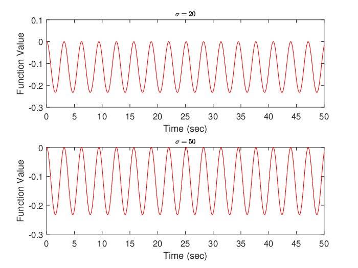
Let (12), (18), (20), and (21) be the updating law with m=−20,σ=20m=-20,\sigma=20, b0=2b_{0}=2, and m=−50,σ=50m=-50,\sigma=50, b0=2b_{0}=2, respectively. The simulation results are shown in Figs. 2-4. Fig. 2 shows the function values calculated by the algorithm when σ=20\sigma=20 and σ=50\sigma=50. Fig. 3 shows the differences of the algorithm function values with the static optimal function value when σ=20\sigma=20 and σ=50\sigma=50 for T=20T=20, i.e., ft​(x⁡(t))−ft​(x~​(20))f_{t}(x(t))-f_{t}(\tilde{x}(20)). Fig. 4 shows the differences of the algorithm function values with the static optimal function value when σ=20\sigma=20 and σ=50\sigma=50 for T=50T=50, i.e., ft​(x⁡(t))−ft​(x~​(50))f_{t}(x(t))-f_{t}(\tilde{x}(50)). The curves are always in the negative half plane. Thus, the conclusion in Theorem 1 is verified.
Refer to caption
Fig. 2: Function values when σ=20\sigma=20 and σ=50\sigma=50.
Refer to caption
Fig. 3: The differences with the static optimal function value when σ=20,T=20\sigma=20,T=20 and σ=50,T=20\sigma=50,T=20.
Refer to caption
Fig. 4: The differences with the static optimal function value when σ=20,T=50\sigma=20,T=50 and σ=50,T=50\sigma=50,T=50.
Refer to caption
Fig. 5: The differences with the dynamic optimal function value when σ=20\sigma=20 and σ=50\sigma=50.
Refer to caption
Fig. 6: The differences with the dynamic optimal function value for eαt+βt−β˙t​eβt=σe^{\alpha_{t}+\beta_{t}}-\dot{\beta}_{t}e^{\beta_{t}}=\sigma and eαt+βt−β˙t​eβt=σ⁡(t+b0)e^{\alpha_{t}+\beta_{t}}-\dot{\beta}_{t}e^{\beta_{t}}=\sigma(t+b_{0}).
Refer to caption
Fig. 7: The differences with the dynamic optimal function value for the continuous-time Online Gradient Descent Methods with a time-varying gain and a time-invariant gain.
Refer to caption
Fig. 8: The difference with the dynamic optimal function value for the discrete-time Online Gradient Descent Method with a step-size 0.67t+1\frac{0.67}{\sqrt{t+1}}.
Refer to caption
Fig. 9: The difference with the dynamic optimal function value for the discrete-time Online Gradient Descent Method with a step-size 1t+1\frac{1}{{t+1}}.
Refer to caption
Fig. 10: The difference with the dynamic optimal function value for the discrete-time Online Gradient Descent Method with a fixed step-size 0.80.8.
Refer to caption
Fig. 11: The difference with the dynamic optimal function value for AdaGrad with η=2\eta=2.
Refer to caption
Fig. 12: The difference with the dynamic optimal function value for FTAL with β=0.02\beta=0.02.

V-A2 Dynamic Regret

We compare the real-time performance of the algorithm with other algorithms according to the difference of the algorithm function value with the dynamic optimal function value i.e., ft​(x⁡(t))−ft​(xt∗)f_{t}(x(t))-f_{t}(x^{*}_{t}). Since it is difficult to obtain an explicit expression of the time-varying optimal solution of the function, in the following comparisons, we select enough discrete-time points and sample the algorithms at these points for comparisons.

Letting (12), (18), (20), and (21) be the updating law, Fig. 5 shows the differences of the algorithm function values with the dynamic optimal function value when σ=20\sigma=20 and σ=50\sigma=50. It can be seen that the error is smaller when σ\sigma is larger.

In the following simulation, we select similar parameters for the algorithms for more precise comparisons. The bound of the gradients is selected to be G=3G=3 and the diameter of the convex set is selected to be D=2D=2 [10, 16].

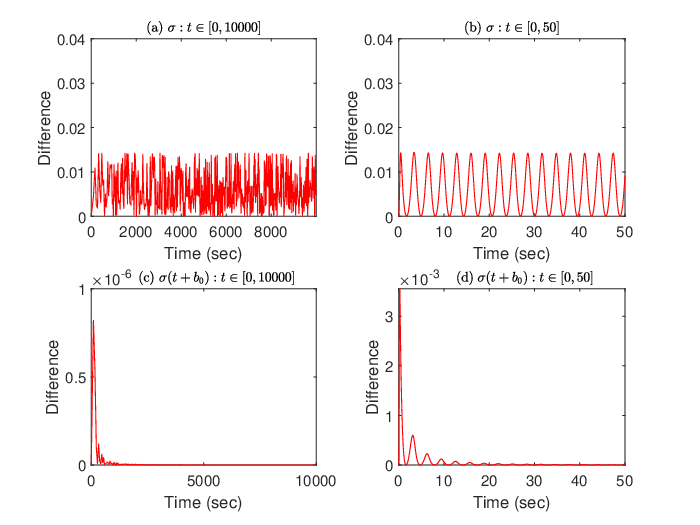
For the algorithm in (12), (18), (20), and (21) which corresponds to the case where eαt+βt−β˙t​eβt=σe^{\alpha_{t}+\beta_{t}}-\dot{\beta}_{t}e^{\beta_{t}}=\sigma, Figs. 6(a) and 6(b) show the algorithm results for 10000​s10000s and 50​s50s, respectively. For the algorithm in (12), (20), (29), and (), which corresponds to the case where eαt+βt−β˙t​eβt=σ⁡(t+b0)e^{\alpha_{t}+\beta_{t}}-\dot{\beta}_{t}e^{\beta_{t}}=\sigma(t+b_{0}), Figs. 6(c) and 6(d) show the results. The parameters are selected to be m=−2,σ=2,b0=2m=-2,\sigma=2,b_{0}=2. It can be seen that the algorithm with eαt+βt−β˙t​eβt=σ⁡(t+b0)e^{\alpha_{t}+\beta_{t}}-\dot{\beta}_{t}e^{\beta_{t}}=\sigma(t+b_{0}) has a better performance.

Fig. 7 shows the differences by using the continuous-time Online Gradient Descent method, where Figs. 7(a) and 7(b) show the case where the gain is selected to be 2t+1\frac{2}{t+1} and Figs. 7(c) and 7(d) show the case where the gain is fixed to be 22.

Fig. 8 shows the difference by using the discrete-time Online Gradient Descent method [10] with a step-size 0.67t+1\frac{0.67}{\sqrt{t+1}} (t=0,1,⋯t=0,1,\cdots). The sampling period for the algorithm is 0.10.1s. The algorithm runs for 100000 steps and a sampling point is selected in every 1000 points to be compared with the dynamic optimal function value.

Fig. 9 shows the difference by using the discrete-time Online Gradient Descent method [10] with a step-size 1t+1.\frac{1}{t+1}.

Fig. 10 shows the difference by using the discrete-time Online Gradient Descent method [10] with a fixed step-size 0.80.8. According to [10], this case can be viewed as a special case of the Online Mirror Descent algorithm in an agile version. Thus, this figure can be viewed as a comparison with the Online Mirror Descent method.

Fig. 11 shows the difference by using the AdaGrad method [10] with parameter η=2\eta=2.

Fig. 12 shows the difference by using the FTAL method [16] with parameter β=0.02\beta=0.02.

It can be seen that for the proposed method with a scaling condition eαt+βt−β˙t​eβt=σ⁡(t+b0)e^{\alpha_{t}+\beta_{t}}-\dot{\beta}_{t}e^{\beta_{t}}=\sigma(t+b_{0}), the upper bound of the difference with the dynamic optimal function value is persistently decreasing (approximately exponentially or polynomially). This phenomenon doesn’t occur in other algorithms. The simulation verifies the effectiveness and efficiency of the proposed algorithm.

V-B DOCT-NAG

In this section, we consider a group of 6 agents that coordinate with each other to solve an optimization problem

min ​ft​(x)=∑i=16fi,t​(x),\displaystyle\text{min }f_{t}(x)=\sum_{i=1}^{6}f_{i,t}(x), (69)

where the decision variable x=[x1,⋯,x6]T∈ℝ6x=[x_{1},\cdots,x_{6}]^{T}\in\mathbb{R}^{6}, and

fi,t​(x)=10​(xT​x+0.2×i×sin​(t)​sin​(xi)).\displaystyle f_{i,t}(x)=10(x^{T}x+0.2\times i\times\text{sin}(t)\text{sin}(x_{i})). (70)

The communication graph of the 6 agents is shown in Fig. 13.

Fig. 13: The communication graph of the 6 agents.

Let 𝐱i∈ℝ6\mathbf{x}_{i}\in\mathbb{R}^{6} be agent ii’s estimation on the optimal solution. Similar to Section V-A, it can be verified that the optimization problem in (69) satisfies Assumptions 5-10.

The initial value of 𝐱\mathbf{x} is selected as 𝐱(0)=[2,1,0,3,0,1,1,1,0,3,0,4,2,1,0,1,0,1,2,1,0,3,0,2,2,1,0,\mathbf{x}(0)=[2,1,0,3,0,1,1,1,0,3,0,4,2,1,0,1,0,1,2,1,0,3,0,2,2,1,0, 3,0,1,2,1,0,0,0,1]T3,0,1,2,1,0,0,0,1]^{T}, and the initial value of 𝐱˙\dot{\mathbf{x}} is zero.

Fig. 14 shows all agents’ estimation on the optimal solution x6,t∗x_{6,t}^{*}. It can be seen that the agents follow the exact optimal solution with high accuracy.

Refer to caption
Fig. 14: The agents’ estimation on the optimal solution x6,t∗x_{6,t}^{*}.

V-B1 Static Regret

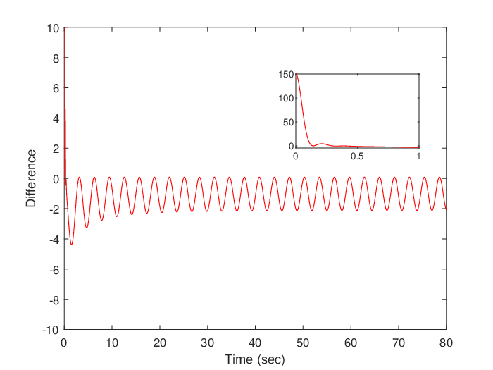
Let (38) be the updating law with (18), (20), (21), (47) and (58), and the parameters being selected as: m=−2,σ=2m=-2,\sigma=2, b0=2b_{0}=2, k1=2k_{1}=2. Fig. 15 shows the difference of the integrated function in the static regret for T=20T=20, i.e., 16​∑j=16∑i=16fi,t​(𝐱j)−∑i=16fi,t​(x~​(20))\frac{1}{6}\sum_{j=1}^{6}\sum_{i=1}^{6}f_{i,t}(\mathbf{x}_{j})-\sum_{i=1}^{6}f_{i,t}({\tilde{x}}(20)), where

x~​(20)=argminx∈ℝ6⁡∫020ft​(x)​𝑑t.\displaystyle\tilde{x}(20)=\mathop{\text{argmin}}\limits_{x\in\mathbb{R}^{6}}\int_{0}^{20}f_{t}(x)dt. (71)

It can be seen that the static regret (the integration of the curve) is upper bounded, which verifies Theorem 4.
Refer to caption
Fig. 15: The difference 16​∑j=16∑i=16fi,t​(𝐱j)−∑i=16fi,t​(x~​(20))\frac{1}{6}\sum_{j=1}^{6}\sum_{i=1}^{6}f_{i,t}(\mathbf{x}_{j})-\sum_{i=1}^{6}f_{i,t}({\tilde{x}}(20)).

V-B2 Dynamic Regret

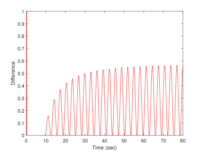
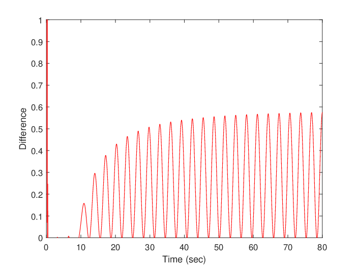
Let (38) be the updating law with (18), (20), (21), (47) and (58), and the parameters being selected as: m=−2,σ=2m=-2,\sigma=2, b0=2b_{0}=2, k1=2k_{1}=2. Fig. 16 shows the difference of the integrated function in the dynamic regret for T=80T=80, i.e., 16​∑j=16∑i=16fi,t​(𝐱j)−∑i=16fi,t​(xt∗)\frac{1}{6}\sum_{j=1}^{6}\sum_{i=1}^{6}f_{i,t}(\mathbf{x}_{j})-\sum_{i=1}^{6}f_{i,t}({x}^{*}_{t}), where eαt+βt−β˙t​eβt=σe^{\alpha_{t}+\beta_{t}}-\dot{\beta}_{t}e^{\beta_{t}}=\sigma. Fig. 17 shows the difference when eαt+βt−β˙t​eβt=σ⁡(t+b0)e^{\alpha_{t}+\beta_{t}}-\dot{\beta}_{t}e^{\beta_{t}}=\sigma(t+b_{0}). It can be seen that the performance is not better when eαt+βt−β˙t​eβt=σ⁡(t+b0)e^{\alpha_{t}+\beta_{t}}-\dot{\beta}_{t}e^{\beta_{t}}=\sigma(t+b_{0}) as the centralized algorithm in Fig. 6.
Refer to caption
Fig. 16: The difference 16​∑j=16∑i=16fi,t​(𝐱j)−∑i=16fi,t​(xt∗)\frac{1}{6}\sum_{j=1}^{6}\sum_{i=1}^{6}f_{i,t}(\mathbf{x}_{j})-\sum_{i=1}^{6}f_{i,t}({x}^{*}_{t}) for eαt+βt−β˙t​eβt=σe^{\alpha_{t}+\beta_{t}}-\dot{\beta}_{t}e^{\beta_{t}}=\sigma.
Refer to caption
Fig. 17: The difference 16​∑j=16∑i=16fi,t​(𝐱j)−∑i=16fi,t​(xt∗)\frac{1}{6}\sum_{j=1}^{6}\sum_{i=1}^{6}f_{i,t}(\mathbf{x}_{j})-\sum_{i=1}^{6}f_{i,t}({x}^{*}_{t}) for eαt+βt−β˙t​eβt=σ⁡(t+b0)e^{\alpha_{t}+\beta_{t}}-\dot{\beta}_{t}e^{\beta_{t}}=\sigma(t+b_{0}).

VI Conclusions

This paper studied the online convex optimization problem by using the proposed OCT-NAG and DOCT-NAG. The online Bregman Lagrangians can generate a family of online optimization algorithms with different scaling conditions. It was shown that for some scaling conditions and under some assumptions, the algorithm achieves a constant static regret and an O⁡(T)O(T) dynamic regret. The algorithm was further applied to solve a distributed online optimization problem. Comparable static and dynamic regrets were obtained. In future, we will work on relaxing the assumptions, discretizing the algorithm, extending the work to stochastic settings and solving constrained optimization problems.

References

  • [1] S. Boyd and L. Vandenberghe, Convex optimization. Cambridge university press, 2004.
  • [2] D. P. Bertsekas, “Nonlinear programming,” Journal of the Operational Research Society, vol. 48, no. 3, pp. 334–334, 1997.
  • [3] Y. Nesterov, “A method of solving a convex programming problem with convergence rate o⁡(1k2)o(\frac{1}{k^{2}}),” in Sov. Math. Dokl, vol. 27, no. 2.
  • [4] ——, Introductory lectures on convex optimization: A basic course. Springer Science & Business Media, 2013, vol. 87.
  • [5] G. Qu and N. Li, “Accelerated distributed nesterov gradient descent,” arXiv preprint arXiv:1705.07176, 2017.
  • [6] T. Tatarenko, W. Shi, and A. Nedić, “Accelerated gradient play algorithm for distributed nash equilibrium seeking,” in 2018 IEEE Conference on Decision and Control (CDC), pp. 3561–3566.
  • [7] W. Su, S. Boyd, and E. Candes, “A differential equation for modeling nesterov’s accelerated gradient method: Theory and insights,” in Advances in Neural Information Processing Systems, 2014, pp. 2510–2518.
  • [8] A. Wibisono, A. C. Wilson, and M. I. Jordan, “A variational perspective on accelerated methods in optimization,” proceedings of the National Academy of Sciences, vol. 113, no. 47, pp. E7351–E7358, 2016.
  • [9] A. Vassilis, A. Jean-François, and D. Charles, “The differential inclusion modeling fista algorithm and optimality of convergence rate in the case b≤3b\leq 3,” SIAM Journal on Optimization, vol. 28, no. 1, pp. 551–574, 2018.
  • [10] E. Hazan et al., “Introduction to online convex optimization,” Foundations and Trends® in Optimization, vol. 2, no. 3-4, pp. 157–325, 2016.
  • [11] A. Y. Popkov, “Gradient methods for nonstationary unconstrained optimization problems,” Automation and Remote Control, vol. 66, no. 6, pp. 883–891, 2005.
  • [12] C. Sun, M. Ye, and G. Hu, “Distributed time-varying quadratic optimization for multiple agents under undirected graphs,” IEEE Transactions on Automatic Control, vol. 62, no. 7, pp. 3687–3694, 2017.
  • [13] S. Rahili and W. Ren, “Distributed continuous-time convex optimization with time-varying cost functions,” IEEE Transactions on Automatic Control, vol. 62, no. 4, pp. 1590–1605, 2017.
  • [14] S. Lee, A. Ribeiro, and M. M. Zavlanos, “Distributed continuous-time online optimization using saddle-point methods,” in 2016 IEEE 55th Conference on Decision and Control (CDC), pp. 4314–4319.
  • [15] M. Zinkevich, “Online convex programming and generalized infinitesimal gradient ascent,” in Proceedings of the 20th International Conference on Machine Learning (ICML-03), 2003, pp. 928–936.
  • [16] E. Hazan, A. Agarwal, and S. Kale, “Logarithmic regret algorithms for online convex optimization,” Machine Learning, vol. 69, no. 2-3, pp. 169–192, 2007.
  • [17] A. Nedic, A. Ozdaglar, and P. A. Parrilo, “Constrained consensus and optimization in multi-agent networks,” IEEE Transactions on Automatic Control, vol. 55, no. 4, pp. 922–938, 2010.
  • [18] S. Liu, Z. Qiu, and L. Xie, “Convergence rate analysis of distributed optimization with projected subgradient algorithm,” Automatica, vol. 83, pp. 162–169, 2017.
  • [19] S. Shahrampour and A. Jadbabaie, “Distributed online optimization in dynamic environments using mirror descent,” IEEE Transactions on Automatic Control, vol. 63, no. 3, pp. 714–725, 2017.
  • [20] S. Hosseini, A. Chapman, and M. Mesbahi, “Online distributed optimization via dual averaging,” in 52nd IEEE Conference on Decision and Control. IEEE, 2013, pp. 1484–1489.
  • [21] D. Mateos-Nunez and J. Cortés, “Distributed online convex optimization over jointly connected digraphs,” IEEE Transactions on Network Science and Engineering, vol. 1, no. 1, pp. 23–37, 2014.
  • [22] A. Koppel, F. Y. Jakubiec, and A. Ribeiro, “A saddle point algorithm for networked online convex optimization,” IEEE Transactions on Signal Processing, vol. 63, no. 19, pp. 5149–5164, 2015.
  • [23] S. Hosseini, A. Chapman, and M. Mesbahi, “Online distributed convex optimization on dynamic networks,” IEEE Transactions on Automatic Control, vol. 61, no. 11, pp. 3545–3550, 2016.
  • [24] E. Takimoto and W. Manfred, “The minimax strategy for gaussian density estimation,” in Proc. 13th Annu. Conference on Comput. Learning Theory, 2000, pp. 100–106.
  • [25] E. C. Hall and R. M. Willett, “Online convex optimization in dynamic environments,” IEEE Journal of Selected Topics in Signal Processing, vol. 9, no. 4, pp. 647–662, June 2015.
  • [26] O. Besbes, G. Yonatan, and Z. Assaf, “Non-stationary stochastic optimization,” Operations Research, vol. 63, no. 5, pp. 1227–1244, 2015.
  • [27] C. Hu, W. Pan, and J. T. Kwok, “Accelerated gradient methods for stochastic optimization and online learning,” in Advances in Neural Information Processing Systems 22, 2009, pp. 781–789.
  • [28] W. Ren and R. W. Beard, “Consensus seeking in multiagent systems under dynamically changing interaction topologies,” IEEE Transactions on Automatic Control, vol. 50, no. 5, pp. 655–661, 2005.
  • [29] A. Simonetto, “Time-varying convex optimization via time-varying averaged operators,” arXiv preprint arXiv:1704.07338, 2017.
  • [30] J. Duchi, E. Hazan, and Y. Singer, “Adaptive subgradient methods for online learning and stochastic optimization,” Journal of Machine Learning Research, vol. 12, no. Jul, pp. 2121–2159, 2011.
  • [31] S. Shalev-Shwartz et al., “Online learning and online convex optimization,” Foundations and Trends® in Machine Learning, vol. 4, no. 2, pp. 107–194, 2012.
  • [32] E. Hazan and S. Arora, Efficient algorithms for online convex optimization and their applications. Princeton University Princeton, 2006.
  • [33] B. Gharesifard and J. Cortés, “Distributed continuous-time convex optimization on weight-balanced digraphs,” IEEE Transactions on Automatic Control, vol. 59, no. 3, pp. 781–786, 2014.
  • [34] S. Liu, Z. Qiu, and L. Xie, “Continuous-time distributed convex optimization with set constraints,” IFAC Proceedings Volumes, vol. 47, no. 3, pp. 9762–9767, 2014.