SWANLOP : Scattering waves off nonlocal optical potentials in the presence of Coulomb interactionsJournal: Computer Physics Communications

H. F. Arellano Corresponding author: Corresponding author.
E-mail address: arellano@dfi.uchile.cl Address: Department of Physics - FCFM, University of Chile, Av. Blanco Encalada 2008, Santiago, Chile Address: CEA,DAM,DIF F-91297 Arpajon, France G. Blanchon Address: CEA,DAM,DIF F-91297 Arpajon, France

Abstract

We introduce the package SWANLOP to calculate scattering waves and corresponding observables for nucleon elastic collisions off spin-zero nuclei. The code is capable of handling local and nonlocal optical potentials superposed to long-range Coulomb interaction. Solutions to the implied Schrödinger integro-differential equation are obtained by solving an integral equation of Lippmann-Schwinger type for the scattering wavefunctions, $\psi=\phi_{{}_{C}}+{G}_{{}_{C}}{U}_{{}_{S}}\psi$ , providing and exact treatment to the Coulomb force [Phys. Lett. B 789, 256 (2019)]. The package has been developed to handle potentials either in momentum or coordinate representations, providing flexible options under each of them. The code is fully self-contained, being dimensioned to handle any $A\!\geq\!4$ target for nucleon beam energies of up to $1.1$ GeV. Accuracy and benchmark applications are presented and discussed.

Keywords:

Scattering wavefunction , Nonlocal optical potential , Nucleon-nucleus scattering , Integro-differential equation, Momentum space , Coulomb potential

Program summary

Program title: SWANLOP
Catalog identifier:
Program summary URL:
Program obtainable from: CPC Program Library, Queen’s University, Belfast, N. Ireland
Licensing provisions: GNU General Public License, Version 2
No. of lines in distributed program, including test data, etc:
No. of bytes in distributed program, including test data, etc:
Distribution format: tar.gz
Programming language: FORTRAN-90
Computer:
Operating system: LINUX, Mac OS
RAM: Memory usage depends on …
Classification:
Nature of problem: Optical model potentials constitute a valuable tool to investigate the physics involved in nuclear collisions and reactions with nucleonic probes. As such, it becomes essential to obtain accurate results for its associated scattering observables and corresponding scattering waves. An important feature of optical potentials is their nonlocal nature, arising from the fermionic nature of the $(\!A\!+\!1)$ –nucleon problem together with the fact that effective nucleon-nucleon (NN) interactions are nonlocal as well. The superposition of Coulomb interaction to these nonlocal potentials poses non-trivial difficulties to obtain scattering waves and observables in collision processes.
Solution method: The code performs the calculation of scattering waves associated to nonlocal potentials in the presence of the long-range Coulomb interactions, solving a Lippmann-Schwinger type integral equation for the scattering wavefunction. The potential can be given either in coordinate or momentum space. Phase-shifts and associated elastic scattering observables are extracted from the asymptotic behavior of the solution.
Running time: The code takes from 1 s, in the case of low-energy nucleon scattering off light targets, up to $100$ s for 1-GeV nucleons off heavy targets, using conventional 2.6 GHz laptop computer.

1 Introduction

Current developments in theoretical nuclear research have set their focus on the development and calculation of non-Hermitian, nonlocal and energy-dependent optical potentials to describe the interaction of nucleonic probes with nuclei. Important achievements in these efforts have been ab-initio approaches reported in Refs. [1, 2], the construction of potentials based on energy density functionals [3, 4, 5], the calculation of $g$ -matrix based optical potentials [6, 7], in addition to $t$ -matrix based optical models [8, 9, 10, 11, 12, 13]. With these advances in mind, the accurate treatment of intrinsic nonlocalities of these potentials in collision processes becomes crucial in order to investigate objectively their physical implications.

In the presence of nonlocal couplings between the projectile and target, Schrödinger equation for scattering waves becomes an integro-differential equation in coordinate space. Furthermore, the superposition of Coulomb interaction to these nonlocal potentials poses non-trivial difficulties to obtain scattering waves and observables in collision processes. In this work we introduce the package SWANLOP aimed to perform such calculations by solving an integral equation for the scattering wavefunction of Lippmann-Schwinger type. The solution to the problem is formally exact as reported in Ref. [14], where the scattering wave gets expressed in terms of known quantities. Optical potentials in momentum representation are treated as well. The resulting scattering waves can further be used in distorted wave Born approximations. The acronym SWANLOP stands for Scattering WAves off NonLocal Optical Potentials.

Several methods have been reported to solve the scattering problem under nonlocal potentials. Early solutions to this problem were proposed by Perey and Buck (PB)[15], where the separable structure of the potential is used to isolate the role of the nonlocal factor, reducing the integro-differential Schrödinger equation into a second-order differential equation with a local coupling. A known disadvantage of this approach is that the resulting scattering waves differ from the exact ones, distortion coined as Perey effect being characterized by a Perey correction factor [16].

Other solutions to Schrödinger’s integro-differential equation follow iterative procedures [15, 16, 17]. In these approaches Schrödinger’s differential equation is integrated with a non-homogeneous term consisting of the projection of the nonlocal coupling onto an intermediate solution. Iterations start with a given seed for the scattering wave, solving Schrödinger equation in the presence of a non-homogeneous term. A drawback of this method is that prior knowledge of the solution is needed for efficient convergence, though there is no theoretical assurance to converge to the actual solution.

In the case of Ref. [18], a mean-value approximation is applied for the coupling of the nonlocal term with the scattering wave, reducing the problem to a second-order homogeneous differential equation. This method is restricted to neutron collisions. Quite recently another approach has been proposed to deal with nonlocal potentials [19], resorting to a Taylor approximation for the radial wave function. The method assumes that nonlocality is dominant around the diagonal in coordinate space, feature which is non universal as observed in coordinate-space representations of potentials originally calculated in momentum space [20].

Solutions to the scattering problem in momentum space have also been investigated [21, 8, 9, 10, 22, 23, 24]. While an appealing advantage of momentum-space approaches is that nonlocalities are naturally accounted for, one of its limitations when long-range Coulomb interactions are included is that the associated scattering waves are not readily available. Not only that, but the long range of the Coulomb interaction results in a $\sim$ $1/q^{2}$ singularity, feature that has led to the use of specific procedures at the moment of calculating scattering amplitudes. An exact solution addressing this singularity has been proposed by Vincent and Phatak by means of a cut-off technique to the Coulomb long-range tail [25]. In this way it is possible to obtain the exact (on-shell) scattering amplitude from the solution for the screened potential. This approach has been applied to proton-nucleus (pA) scattering at intermediate energies [8], where its accuracy is significantly improved after a detailed multipole treatment of the charge form factor convoluted with a sharp cut-off point Coulomb potential, as discussed by Einsenstein and Tabakin [26].

In works by Alt et al. [27, 28] the Coulomb long-range potential is screened with the use of smooth radial form factors, resulting in finite-range interactions. The associated scattering matrix can then be calculated using standard techniques. The zero-screening limit is obtained by increasing the range $R$ of the form factor in conjunction with the use of renormalization factors. This method has been refined by Deltuva and collaborators [29, 30] in studies of three-nucleon breakup reactions in momentum space. In their work exponential screening form factors of type $\sim\!\exp[-(r/R)^{4}]$ are used.

Studies pursued by Elster and collaborators [31, 22, 32] have addressed the pA scattering problem without resorting to screening techniques. Here the full pA interaction is re-expressed as the sum of a point Coulomb term and short-range residuum. The use of two-potential formalism enables to express the scattering amplitude as the sum of two terms. A residual Coulomb-modified transition matrix is obtained solving a Lippmann-Schwinger equation for a modified potential which includes Coulomb distortions. Calculated scattering observables for pA scattering are accurate even for 500-MeV protons off heavy targets.

Another method to calculate waves off nonlocal potentials in the presence of long-range Coulomb interaction is that of Refs. [33, 34], where Lanczos technique is used to solve integral equations derived from the nonlocal Schrödinger equation. Later on, in Refs. [35, 36] a numerical treatment to this problem is presented with the use of Berggren basis, where an off-diagonal approximation is used to control the Coulomb singularity along the diagonal in momentum space. Applications of this approach have been reported for low energies and intermediate-mass targets.

Quite recently the package SIDES (Schrödinger Integro-Differential Equation Solver) has been introduced [37], featuring an exact treatment of the long-range Coulomb interaction. The approach is based on finite difference techniques [38, 39], where the integro-differential equation in coordinate space is reduced to a matrix equation for the wavefunction. This approach contrasts with the method we use in SWANLOP, where wavefunctions are obtained from an integral equation for the wavefunction, including Coulomb interactions. Additionally, SWANLOP features the possibility of working with potentials given in momentum space.

This paper is organized as follows. In Sec. 2 we lay out the framework and present a formal solution to the scattering problem with nonlocal potentials in the presence of Coulomb interactions. We also establish contact with potentials represented in momentum space, providing transformation into coordinate representation, to obtain exact scattering observables in the presence of Coulomb interaction. In Sec. 3 we describe the SWANLOP package, its I/O structure, main options and execution of the code. In Sec. 4 we study the accuracy of SWANLOP by comparing with analytic solutions, exploring convergence on integration step length and comparing results with the recently released package SIDES [37]. Additionally, we discuss CPU run-time performance of the code. In Sec. 5 we present a summary and conclusions of this work.

2 Framework

In this section we layout key equations needed to describe NA collisions under nonlocal potentials (in coordinate space) superposed to Coulomb forces. We present the solution to the scattering problem and make contact with potentials expressed in momentum representation. For details on the derivation of the solution we refer the reader to Ref. [14].

Consider a proton of mass $m$ with kinetic energy $E_{lab}$ in the laboratory reference frame, colliding a spin-zero nucleus of mass $M$ and charge $Ze$ at rest. Let $U$ the full interaction between them, being comprised of a pure hadronic contribution $U_{H}$ and Coulomb interaction $V_{{}_{C}}$ due to the distributed charge in the nucleus. The hadronic part is short-range so that the total interaction can be cast as the sum of point-Coulomb and short-range terms,

U({\bm{r}}^{\prime},{\bm{r}})=U^{(s)}({\bm{r}}^{\prime},{\bm{r}})+\frac{\beta}{r}\,\delta({\bm{r}}^{\prime}-{\bm{r}})\;,

(1)

with $\beta=Ze^{2}$ . Here $U^{(s)}\!=\!U_{H}\!+\!V_{{}_{C}}\!-\!\beta\,\delta({\bm{r}}^{\prime}-{\bm{r}})/r$ , which vanishes rapidly away from the nucleus. In the case of neutron scattering both $\beta$ and $V_{{}_{C}}$ vanish, so that $U^{(s)}\!=\!U_{H}$ , being this a particular case in the discussion that follows.

With the above Schrödinger’s equation for scattering waves in the center-of-momentum reference frame reads

-\nabla^{2}\psi_{\bm{k}}({\bm{r}})+\frac{2\mu}{\hbar^{2}}\int d{\bm{r}^{\prime}}U({\bm{r}},{\bm{r}^{\prime}})\psi_{\bm{k}}({\bm{r}^{\prime}})=k^{2}\psi_{\bm{k}}({\bm{r}})\;,

(2)

where $\mu$ denotes the NA reduced mass and $k$ the asymptotic relative momentum in the NA center-of-momentum reference frame. We omit spin and isospin variables for simplicity in the notation. Consistent with spin $-\nicefrac{{1}}{{2}}$ nucleons colliding a spherical target we expand

\psi_{\bm{k}}({\bm{r}})=\sqrt{\frac{2}{\pi}}\;\sum_{jlm_{j}}i^{l}{\cal Y}_{jl1/2}^{m_{j}}({\hat{\bm{r}}})e^{i\sigma_{l}}\frac{u_{jl}(r)}{r}{\cal Y}_{jl1/2}^{m_{j}\dagger}({\hat{\bm{k}}})\;.

(3)

Here $u_{jl}(r)$ denotes the radial wavefunction and $\sigma_{l}$ the Coulomb phase-shift for partial wave $l$ . Furthermore, $\mathcal{Y}_{jls}^{m_{j}}$ stand for spin $s\!=\!\nicefrac{{1}}{{2}}$ spherical vectors

\mathcal{Y}_{jls}^{m_{j}}(\hat{\bm{k}})=\sum_{mm_{s}}Y_{l}^{m}(\hat{\bm{k}})\,|sm_{s}\rangle\langle ls\,mm_{s}|jm_{j}\rangle\,.

(4)

The normalization adopted in Eq. (3) for $\psi_{\bm{k}}({\bm{r}})$ is such that it reduces to normalized plane waves $\sim\!e^{i{\bm{k}}\cdot{\bm{r}}}/(2\pi)^{3/2}$ , when interactions are fully suppressed.

Replacing $\psi_{\bm{k}}({\bm{r}})$ from Eq. (3) into Eq. (2), following standard procedures we get

\left[\frac{1}{r}\left(\frac{d^{2}}{dr^{2}}\right)r-\frac{l(l+1)}{r^{2}}+k^{2}\right]\frac{u_{jl}(r)}{r}=\frac{2\mu}{\hbar^{2}}\int_{0}^{\infty}r^{\prime}\,dr^{\prime}U_{jl}(r,r^{\prime})u_{jl}(r^{\prime})\;,

(5)

where the multipoles $U_{jl}(r^{\prime},r)$ of the interaction are obtained from

U_{jl}(r^{\prime},r)=\iint d\hat{\bm{r}}\,d\hat{\bm{r}}^{\prime}{\cal Y}_{jl1/2}^{m_{j}\dagger}({\hat{\bm{r}}}^{\prime})U({\bm{r}^{\prime}},{\bm{r}}){\cal Y}_{jl1/2}^{m_{j}}(\hat{\bm{r}})\;.

(6)

Making explicit the separation of the interaction into a pointlike source and finite-range remaining

U_{jl}(r^{\prime},r)\equiv U_{jl}^{(s)}(r^{\prime},r)+\frac{\beta}{r^{3}}\delta(r^{\prime}-r)\;,

(7)

we obtain

\left[\frac{d^{2}}{dr^{2}}-\frac{l(l+1)}{r^{2}}-\frac{2k\eta}{r}+k^{2}\right]u_{jl}(r)=\frac{2\mu}{\hbar^{2}}\int_{0}^{\infty}dr^{\prime}rU_{jl}^{(s)}(r,r^{\prime})r^{\prime}u_{jl}(r^{\prime})\;,

(8)

with $\eta$ the Sommerfeld parameter given by $\eta\!=\!\mu\beta/\hbar^{2}k$ . Following Ref. [14], a formal solution to this equation is expressed as the superposition of homogeneous and particular solutions in the form

u_{jl}(r)=\frac{1}{k}F_{l}(\eta,kr)+\frac{2\mu}{\hbar^{2}}\iint dr^{\prime}dr^{\prime\prime}G_{l}^{c(+)}(r,r^{\prime};k)\left[r^{\prime}U^{(s)}_{jl}(r^{\prime},r^{\prime\prime})r^{\prime\prime}\right]u_{jl}(r^{\prime\prime})\;,

(9)

with the Coulomb propagator

G_{l}^{c(+)}(r,r^{\prime};k)=-\frac{i}{k}F_{l}(\eta,kr_{<})\left[F_{l}(\eta,kr_{>})-iG_{l}(\eta,kr_{>})\right]\;,

(10)

where $r_{<}\!=\!\textrm{min}(r,r^{\prime})$ , and $r_{>}\!=\!\textrm{max}(r,r^{\prime})$ . In the above $F_{l}$ and $G_{l}$ denote regular and irregular Coulomb functions [40] under the phase convention

	$\displaystyle F_{l}(\eta,z)$	$\displaystyle\xrightarrow[\;z\to\infty]{}\sin(z-\eta\ln 2z-l\pi/2+\sigma_{l})\;,$
	$\displaystyle G_{l}(\eta,z)$	$\displaystyle\xrightarrow[\;z\to\infty]{}\cos(z-\eta\ln 2z-l\pi/2+\sigma_{l})\;.$		(11)

Note that the Coulomb propagator expressed by Eq. (10) is non-singular, being a continuous function of $r$ and $r^{\prime}$ . The spatial gradient of $G_{l}^{c(+)}(r^{\prime},r;k)$ is discontinuous at the diagonal $r\!=\!r^{\prime}$ , feature that poses no particular drawback. Furthermore, Eq. (9) takes the form of an integral equation for scattering waves in the presence of Coulomb interaction, which we recast as

\int_{0}^{\infty}dr^{\prime\prime}\left[\delta(r-r^{\prime\prime})-K_{jl}(r,r^{\prime\prime})\right]u_{jl}(r^{\prime\prime})=\textstyle{\frac{1}{k}}F_{l}(\eta,kr)\;,

(12)

where the kernel $K_{jl}$ is given by

K_{jl}(r,r^{\prime\prime})=\frac{2\mu}{\hbar^{2}}\int_{0}^{\infty}dr^{\prime}G_{l}^{c(+)}(r,r^{\prime};k)\left[r^{\prime}U^{(s)}_{jl}(r^{\prime},r^{\prime\prime})r^{\prime\prime}\right]\;.

(13)

Note that Eq. (12) enables to obtain the actual scattering wavefunction by means of direct matrix inversion.

The solution for $u_{jl}$ from Eq. (12) enables the calculation of the scattering amplitude, which follows from the asymptotic form of Eq. (9), where $r$ is taken far away from the scattering center. In this limit we have

G_{l}^{c(+)}(r,r^{\prime};k)\xrightarrow[r\gg r^{\prime}]{}-\frac{i}{k}F_{l}(\eta,kr^{\prime})\left[F_{l}(\eta,kr)-iG_{l}(\eta,kr)\right]\;,

(14)

which once replaced in Eq. (9) for $u_{jl}$ yields

k\,u_{jl}(r)\xrightarrow[r\to\infty]{}F_{l}(\eta,kr)+\Delta_{jl}\left[F_{l}(\eta,kr)-iG_{l}(\eta,kr)\right],

(15)

with

\Delta_{jl}=-\frac{2\mu i}{\hbar^{2}}\iint r^{\prime}dr^{\prime}\,r^{\prime\prime}dr^{\prime\prime}F_{l}(\eta,kr^{\prime})U^{(s)}_{jl}(r^{\prime},r^{\prime\prime})u_{jl}(r^{\prime\prime})\;.

(16)

These last two relations allow independent ways to obtain $\Delta_{jl}$ . The latter involves direct integration of the wavefunction whereas the former evaluates asymptotically the ratio

\Delta_{jl}=\frac{ku_{jl}(r)-F_{l}(\eta,kr)}{F_{l}(\eta,kr)-iG_{l}(\eta,kr)}\;,

(17)

for sufficiently large $r$ . These last two equivalent forms for $\Delta_{jl}$ are useful for consistency checks. Once $\Delta_{jl}$ is obtained, the scattering amplitude $f_{jl}$ and short-range phase shift $\bar{\delta}_{jl}$ follow from

\Delta_{jl}=ikf_{jl}=\textstyle{\frac{1}{2}}\left(e^{2i\bar{\delta}_{jl}}-1\right).

(18)

Later on it will be useful to refer to the $S$ matrix associated to $\bar{\delta}_{jl}$ , defined by

\bar{S}_{jl}=e^{2i\bar{\delta}_{jl}}\;.

(19)

The numerical implementation of Eq. (12) follows from the discretization of $r$ (and $r^{\prime\prime}$ ) over an $N$ -point uniform mesh up to $r\!=\!R_{max}$ . The $n$ -th element of this array is given by $r_{n}\!=\!n\,h$ , with $h\!=\!R_{max}/N$ . We find trapezoidal rule adequate to evaluate the integrals. The kernel in Eq. (13), function of $r$ and $r^{\prime}$ , becomes a finite $N\!\times\!N$ matrix which we denote by $\mathbb{K}$ . This kernel is fully determined by the matrix elements of the potential and free Coulomb functions, all of them known quantities. The solution to Eq. (12) takes the form

\textrm{\bf u}=(1-\mathbb{K})^{-1}\textrm{\bf u}_{0}\;,

(20)

where $\textrm{\bf u}_{0}$ represents the unperturbed wave $F_{l}(\eta,kr)/k$ , and u denotes the scattering wave over the discrete mesh. In this way the scattering wavefunction is directly determined by inverting a known matrix, which is then multiplied to a known vector. There is no need to introduce normalization constants nor the calculation of derivatives to match asymptotic behaviors [14].

2.1 Potential in momentum space

This section is aimed to provide explicit relationships between potentials represented in momentum space, with their coordinate space counterparts $U_{jl}(r^{\prime},r)$ in Eq. (13) for the kernel. As already mentioned, microscopic optical model potentials in momentum space have the appealing feature of incorporating in a natural way intrinsic nonlocalities in $(\!A\!+\!1)$ –nucleon systems. Calculations of these potentials are performed in momentum space by folding the ground-state mixed density with an effective interaction. At intermediate nucleon energies, the NN effective interaction can be taken as the free $t$ matrix [8, 9, 10, 11, 12]. At lower energies the use of the density-dependent Brueckner-Bethe-Goldstone $g$ matrix becomes suitable [6, 41]. In all these approaches the optical potential for NA elastic scattering, $\tilde{U}({\bm{k}}^{\prime},{\bm{k}};E)$ , can be cast in the form

\tilde{U}({\bm{k}^{\prime}},{\bm{k}})=\tilde{U}_{0}({\bm{k}^{\prime}},{\bm{k}})+i{\bm{\sigma}}\cdot\hat{\bm{n}}\,\tilde{U}_{1}({\bm{k}^{\prime}},{\bm{k}})\;,

(21)

with $\hat{\bm{n}}$ the unit vector perpendicular to the scattering plane given by

\hat{\bm{n}}=\frac{\bm{k}^{\prime}\times\bm{k}}{|\bm{k}^{\prime}\times\bm{k}|}\,,

(22)

and ${\bm{\sigma}}$ the spin of the projectile. Here $\tilde{U}_{0}$ and $\tilde{U}_{1}$ represent central and spin-orbit components of the potential, which we assume calculated over a grid of relative momenta, $k$ and $k^{\prime}$ , and angles between ${\bm{k}}$ and ${\bm{k}}^{\prime}$ expressed by $u\!=\!\hat{\bm{k}}\cdot\hat{\bm{k}}^{\prime}$ . With these considerations in mind, we express $\tilde{U}_{0}\!=\!\tilde{U}_{0}(k^{\prime},k;u)$ , and $\tilde{U}_{1}\!=\!\tilde{U}_{1}(k^{\prime},k;u)$ . In what follows we seek the relationship between these two terms and $U_{jl}(r^{\prime},r)$ needed in Eq. (5) to obtain its associated scattering waves.

Consistent with Eq. (6), let us expand

\tilde{U}(\bm{k}^{\prime},\bm{k})=\sum_{jm_{j}l}\mathcal{Y}_{jls}^{m_{j}}(\hat{\bm{k}}^{\prime})\tilde{U}_{jl}(k^{\prime},k)\mathcal{Y}_{jls}^{m_{j}\dagger}(\hat{\bm{k}}),

(23)

Let us also consider the identity

\sum_{m_{j}=-j}^{j}\mathcal{Y}_{jls}^{m_{j}}(\hat{\bm{k}}^{\prime})\mathcal{Y}_{jls}^{m_{j}\dagger}(\hat{\bm{k}})=\frac{(2j+1)}{8\pi}\left[\rule[18.0pt]{0.0pt}{0.0pt}P_{l}(u)\mathbb{1}_{\sigma}+\right.\left.i{\bm{\sigma}}\cdot\hat{\bm{n}}\,\frac{\langle{\bm{\ell}}\cdot{\bm{\sigma}}\rangle_{jl}}{l(l+1)}\,P_{l}^{1}(u)\right],

(24)

with $P_{l}^{1}(u)=\sqrt{1-u^{2}}\,dP_{l}(u)/du$ , the associated Legendre polynomia. Additionally, $\langle{\bm{\ell}}\cdot{\bm{\sigma}}\rangle_{jl}=j(j+1)-l(l+1)-\nicefrac{{3}}{{4}}$ . Combining Eqs. (21), (23) and (24) we identify


$\displaystyle\tilde{U}_{0}(k^{\prime},k;u)$	$\displaystyle=\sum_{jl}\frac{(2j+1)}{8\pi}\tilde{U}_{jl}(k^{\prime},k)\,P_{l}(u)$	(25a)
$\displaystyle\tilde{U}_{1}(k^{\prime},k;u)$	$\displaystyle=\sum_{jl}\left[\frac{(2j+1)\langle{\bm{\ell}}\cdot{\bm{\sigma}}\rangle_{jl}}{8\pi\;l(l+1)}\right]\tilde{U}_{jl}(k^{\prime},k)\,\,P_{l}^{1}(u)\;.$	(25b)

Using orthogonality of Legendre polynomia we get


$\displaystyle\sum_{j=l-1/2}^{l+1/2}\frac{(2j+1)}{(2l+1)}\tilde{U}_{jl}(k^{\prime},k)$	$\displaystyle=4\pi\int_{-1}^{1}\tilde{U}_{0}(k^{\prime},k;u)\,P_{l}(u)\,du$	(26a)
$\displaystyle\sum_{j=l-1/2}^{l+1/2}\frac{(2j+1)\langle{\bm{\ell}}\cdot{\bm{\sigma}}\rangle_{jl}}{(2l+1)}\tilde{U}_{jl}(k^{\prime},k)$	$\displaystyle=4\pi\int_{-1}^{1}\tilde{U}_{1}(k^{\prime},k;u)\,P_{l}^{1}(u)\,du\;.$	(26b)

From these two equations we obtain

U_{jl}(k^{\prime},k)=M_{l}^{(0)}(k^{\prime},k)+\frac{\langle{\bm{\ell}}\cdot{\bm{\sigma}}\rangle_{jl}}{l(l+1)}\,M_{l}^{(1)}(k^{\prime},k)\;,

(27)

where


$\displaystyle M_{l}^{(0)}(k^{\prime},k)$	$\displaystyle=2\pi\int_{-1}^{1}\tilde{U}_{0}(k^{\prime},k;u)\,P_{l}(u)\,du$	(28a)
$\displaystyle M_{l}^{(1)}(k^{\prime},k)$	$\displaystyle=2\pi\int_{-1}^{1}\tilde{U}_{1}(k^{\prime},k;u)\,P_{l}^{1}(u)\,du\;.$	(28b)

With $\tilde{U}_{jl}(k^{\prime},k)$ given by Eq. (27) we proceed to obtain its coordinate-space counterpart, which we expand as

U(\bm{r}^{\prime},\bm{r})=\sum_{jm_{j}l}\mathcal{Y}_{jls}^{m_{j}}(\hat{\bm{r}}^{\prime})U_{jl}(r^{\prime},r)\mathcal{Y}_{jls}^{m_{j}\dagger}(\hat{\bm{r}}).

(29)

Using normalized plane waves

\langle{\bm{r}}|{\bm{k}}\rangle=\frac{e^{i{\bm{k}}\cdot{\bm{r}}}}{(2\pi)^{3/2}}\,=\sqrt{\frac{2}{\pi}}\sum_{lm}Y_{l}^{m}(\hat{\bm{r}})i^{l}j_{l}(kr)Y_{l}^{m*}(\hat{\bm{k}}),

(30)

we evaluate

U({\bm{r}}^{\prime},{\bm{r}})=\iint d{\bm{k}}^{\prime}d{\bm{k}}\langle{\bm{r}}^{\prime}|{\bm{k}}^{\prime}\rangle\,\tilde{U}({\bm{k}^{\prime}},{\bm{k}})\,\langle{\bm{k}}|{\bm{r}}\rangle,

(31)

to obtain

r^{\prime}U_{jl}(r^{\prime},r)r=\frac{2}{\pi}\!\int_{0}^{\infty}\!\!dk^{\prime}\!\int_{0}^{\infty}\!\!dk\,{\cal S}_{l}(k^{\prime}r^{\prime})\,k^{\prime}\tilde{U}_{jl}(k^{\prime},k)k\,{\cal S}_{l}(kr),

(32)

where ${\cal S}_{l}$ denotes Riccati-Bessel functions given by ${\cal S}_{l}(x)\!=\!xj_{l}(x)$ .

To summarize the passage of momentum- to coordinate-space representation of potentials, starting from known values of the central and spin-orbit terms in momentum space, $\tilde{U}_{0}(k^{\prime},k;u)$ and $\tilde{U}_{1}(k^{\prime},k;u)$ , we use Eqs. (28a) and (28b) to obtain $\tilde{U}_{jl}(k^{\prime},k)$ in Eq.(27). The passage to coordinate space is completed with the double Fourier transform expressed by Eq. (32). The resulting potential is then used to evaluate the kernel in Eq. (12) to obtain scattering waves. In the above, we denote $\tilde{U}_{0}(k^{\prime},k;\cos\theta)\!\equiv\!\tilde{U}_{0}(k^{\prime},k,\theta)$ , with analogous notation for $\tilde{U}_{1}$ .

To evaluate the volume integral $J$ of the potential from its momentum-space representation $\tilde{U}$ we use Eq. (31), leading to

J=(2\pi)^{3}\;\tilde{U}({\bm{k}}^{\prime}\!=\!0,{\bm{k}}\!=\!0)\;.

(33)

Thus, the volume integral of the potential is proportional to its value in momentum space at ${\bm{k}^{\prime}}\!=\!{\bm{k}}\!=\!0$ . Consistently, in coordinate representation we obtain

J=4\pi\int_{0}^{\infty}r^{\prime 2}dr^{\prime}\int_{0}^{\infty}r^{2}\,drU_{j0}(r^{\prime},r)\;,

(34)

with $j\!=\!\nicefrac{{1}}{{2}}$ . These two forms of $J$ are calculated by the code.

2.2 Elastic scattering observables

Here we spell out the formulas used to evaluate the scattering observables. Considering collisions of spin- $\nicefrac{{1}}{{2}}$ nucleons with spin- $0$ target, the differential cross section for unpolarized-beam NA scattering is given by

\dfrac{d\sigma}{d\Omega}=|g(\theta)|^{2}+|h(\theta)|^{2},

(35)

with the scattering amplitudes $g(\theta)$ and $h(\theta)$ given by


$\displaystyle g(\theta)$	$\displaystyle=f_{{}_{C}}(\theta)+\frac{i}{4k}\sum_{l=0}^{\infty}\sum_{j}(2j+1)e^{2i\sigma_{l}}(1-\bar{S}_{jl})P_{l}(\cos\theta)$	(36a)
$\displaystyle h(\theta)$	$\displaystyle=-\frac{1}{2k}\sum_{l=1}^{\infty}\sum_{j}C_{jl}\,e^{2i\sigma_{l}}(1-\bar{S}_{jl})\,\frac{\partial P_{l}(\cos\theta)}{\partial\theta}\;.$	(36b)

Summations over $j$ range from $|l\!-\!\nicefrac{{1}}{{2}}|$ to $(l\!+\!\nicefrac{{1}}{{2}})$ . In the above, $\theta$ corresponds to the center-of-momentum deflection angle of the projectile, $P_{l}$ denotes Legendre polynomial, and coefficient $C_{jl}$ given by

C_{jl}=\frac{(2j+1)\langle\sigma\cdot\ell\rangle_{jl}}{2l(l+1)}=\left\{\begin{array}[]{rl}-1&\textrm{for $j=l-\nicefrac{{1}}{{2}}$};\\ +1&\textrm{for $j=l+\nicefrac{{1}}{{2}}$}.\\ \end{array}\right.

(37)

Additionally, Coulomb amplitude $f_{{}_{C}}(\theta)$ is given by

f_{C}(\theta)=\frac{-\eta}{2k\sin^{2}(\theta/2)}\;\exp\{-i\eta\ln[\sin^{2}(\theta/2)]+2i\sigma_{0}\}\;.

(38)

Scattering experiments using polarized beams allow measurements of analyzing power $A_{y}$ and spin rotation function $Q$ . These quantities are calculated by SWANLOP from

A_{y}(\theta)+i\,Q(\theta)=\frac{2\,g^{*}(\theta)\,h(\theta)}{|g(\theta)|^{2}+|h(\theta)|^{2}}\,.

(39)

Total (integrated) cross sections are evaluated with


$\displaystyle\sigma_{{}_{R}}$	$\displaystyle=\frac{\pi}{2k^{2}}\sum_{l=0}^{\infty}\sum_{j}(2j+1)\left(1-\left\|S_{jl}\right\|^{2}\right)\;;$	(40a)
$\displaystyle\sigma_{{}_{E}}$	$\displaystyle=\frac{\pi}{2k^{2}}\sum_{l=0}^{\infty}\sum_{j}(2j+1)\left\|1-S_{jl}\right\|^{2}\;;$	(40b)
$\displaystyle\sigma_{{}_{T}}$	$\displaystyle=\frac{\pi}{k^{2}}\sum_{l=0}^{\infty}\sum_{j}(2j+1)\left(1-\mathrm{Re}\{S_{jl}\}\right)\;.$	(40c)

Here $\sigma_{{}_{R}}$ , $\sigma_{{}_{E}}$ and $\sigma_{{}_{T}}$ denote reaction, shape-elastic and total cross sections, respectively. In these expressions $S_{jl}\!=\!\exp[2i(\sigma_{l}+\bar{\delta}_{jl})]$ . For proton scattering only the reaction cross section is meaningful, as both $\sigma_{{}_{E}}$ and $\sigma_{{}_{T}}$ diverge with increasing number of partial waves.

2.3 General considerations

Calculations performed by SWANLOP allow for nucleon energies of up to $1.1$ GeV. Thus, relativistic corrections of kinematical nature need to be implemented. A brief description of these corrections are given in A. Additionally, proton collisions require the inclusion of Coulomb interactions. The model we use is that due to a uniform charge distribution as described in B. However, the specific subroutine for Coulomb potential evaluation can be customized to meet specific requirements.

As guiding rule for the maximum radius of integration, $R_{max}$ , we follow the prescription

R_{max}=r_{0}A^{1/3}+\bar{R}\;,

(41)

with $r_{0}\!=\!1.2$ fm, $\bar{R}\!=\!8$ fm, and $A$ the mass number of the target. This sets the maximum integration radius about 8 fm further away from the surface of the target. With respect to the maximum orbital angular momentum to be considered we follow the rule

L_{max}\sim k\,R_{max}\;,

(42)

with $k$ the c.m. momentum. With the above, collisions of 1 GeV protons off ²²⁶Ra would lead to $R_{max}\!\approx\!16$ fm, with $L_{max}\!=\!130$ . We stress that these are guiding rules. Actual values for $R_{max}$ and $L_{max}$ may depend on specific features of the potential together with the needed precision of observables under study.

Another important consideration is the radial step length $h$ to be used by the code to solve the scattering problem. Here we expect a spatial oscillatory behavior for the wavefunction, as driven by the c.m. wavenumber $k$ . In order to keep track of these oscillations we impose that each cycle is sampled a certain number of times, feature which accommodates well to the trapezoidal quadrature in the radial coordinate. Keeping control on the dimension matrices to be inverted together with reasonable accuracy in the calculated observables, we have found that half-cycles of the free waves being sampled by at least six points yields acceptable accuracy. With this empirical rule we estimate

h\lesssim\frac{\pi}{6\,k}\;,

(43)

condition checked by the program which issues a warning message if not met. Thus, for a given $R_{max}$ the value of $h$ is controlled by the dimension $N$ of the matrix representing the kernel in Eq. (13).

An element which also conditions the value of $h$ is the nature of the potential. As demonstrated in Ref. [20], microscopic momentum-space potentials when transformed into coordinate representation exhibit strong oscillating patterns. The roughness of these patterns depends on the upper momentum at which they are defined in momentum space. Interestingly, a reduction (via cut off) of the upper momenta of the potential yields smoother nonlocal potentials with the same scattering observables and wavefunctions. In the context of Schrödinger’s wave equation, these smoother nonlocal potentials become computationally less demanding in terms of the step size $h$ .

3 The package SWANLOP

The package is distributed in a single tarred and zipped file named swanlop.tar.gz. To unwrap the package apply the command:
tar -xvfz swanlop.tar.gz
This action will create the directory SWANLOP/ containing the following file and subdirectories:

1.

./README
containing instructions to setup the program, prepare inputs and run instructions;
2.

./sources/
subdirectory containing the main program swanlop.f, twenty-six subroutines and twelve functions written in Fortran 90. Additionally, it contains a makefile and the executable file;
3.

./runs/
subdirectory for inputs, outputs and code execution; and
4.

./udata/
subdirectory containing input potentials for testing and reference.

The SWANLOP package is self-contained, independent of any library. To compile the code, once at subdirectory ./SWANLOP/sources/ type make followed by return key. This action will create the executable swanlop.x at ./SWANLOP/sources/

3.1 Data

Fundamental constants and unified atomic mass units are stored in file include_ phys at subdirectory ./SWANLOP/sources/. Their values are

$\hbar c\!=$ $197.326\,978\,8$ MeV fm	Conversion constant [42]
$\alpha\!=$ $1\text{/}137.035\,999$	Fine-structure constant [42]
$u\!=$ $931.494\,095$ MeV/ $c^{2}$	Unified atomic mass unit [43]

Whenever any of these values is modified delete all *.o files and re-compile. Additionally, file NucChart at subdirectory ./SWANLOP/runs/ stores mass excess data of $3436$ nuclides, to obtain masses of the colliding particles during runs. This data basis has been obtained from The AME2016 atomic mass evaluation [43, 44].

Input files to be prepared by the user to run the code are the following:

fort.1:	main input with run specifications;
fort.2:	(optional) external nonlocal potential; and
fort.22:	(optional) external local potential.

Follow instructions given at SWANLOP/runs/README to construct fort.1 according to specified requirements. Further explanations are given in Sec. 3.3.

3.2 Execution

The execution of the program is performed at subdirectory ./SWANLOP/runs/, typing

../sources/swanlop.x

followed by return key. After execution, SWANLOP generates three outputs by default, with two additional (optional) outputs if specified. These outputs are zz.main, zz.xaq, zz.dsdt, zz.wave and zz.vrr, to be described in Sec. 3.4.

3.3 Input files

3.3.1 Main input

The main input file is fort.1, consisting of sixteen lines listed in Table 1, where we maintain the notation used in the main code swanlop.f. For the HEADING entry use any US keyboard character, excepting empty spaces, slashes (/), semicolons (;) and commas (,) as they may trim off any text after their occurrence. The collision is defined with entries PROJ, TARGET and ELAB, defining the projectile, target and nucleon beam energy, respectively. Radial integration specifications are given by RMAX and NRP, representing $R_{max}$ and $N$ in Eq. (20). The maximum orbital angular momentum $L_{max}$ is specified by LMAX. We refer the reader to C for considerations on these three entries when potentials are read from file.

Line	Entry	Type	Meaning	Values
1	HEADING	Character	Unbroken 70-character job title
2	PROJ	Character	Projectile	$p$ or $n$
3	TARGET	Character	Target specification	e.g. Ca40
4	ELAB	Real	Nucleon beam energy $E_{lab}$
5	RMAX	Real	Maximum integration radius $R_{max}$
6	NRP	Integer	Number of radial points $N$
7	LMAX	Integer	Maximum angular momentum $L_{max}$
8	ANGMAX,DANG	Real	Angular array [deg] for $d\sigma\!/\!d\Omega$	ANGMAX $\leq\!180$
9	KIN	Integer	Relativistic kinematics	0(no) 1(yes)
10	KPOT	Integer	Potential specification	0, 1, 2, 3 or 4
11	KADD	Integer	Addition of local potential	0(none) 1(read) 2(call)
12	KPRwave	Integer	Print wavefunctions	0(no) 1(yes)
13	KPRvrr	Integer	Print nonlocal potential	0(no) 1(yes)
14	DATdsdw	Character*18	Filename for $d\sigma/d\Omega$ data	none if none
15	DATay	Character*18	Filename for $A_{y}$ data	none if none
16	DATqrot	Character*18	Filename for $Q$ data	none if none

Table 1: Entries in fort.1 to specify the main task.

Parameters ANGMAX and DANG at line 8 specify the angular array for the c.m. angle $\theta$ over which angular scattering observables are to be evaluated. Entries are given in degrees, with ANGMAX the maximum scattering angle $\theta$ and DANG the angular step. If ANGMAX $<\!0$ , the program sets the grid internally. Entry KIN defines the kinematics to be applied in the NA collision. When KIN=1, relativistic kinematics is used as described in A.

Entry KPOT at line 10 defines the potential to be considered in the run. The allowed values and meaning are summarized in Table 2. We note that under choices KPOT=1,2, the optical potential is generated internally by the code, using PB optical model [15] or Tian-Pang-Ma (TPM) parametrization [45] of PB model. The option to superpose a local potential to nonlocal ones is explained in Sec. 3.3.3.

KPOT	Meaning
0	For purely local potential read from file
1	For Perey-Buck nonlocal model
2	For TPM parametrization in PB-type model
3	For coordinate-space nonlocal potential read from file
4	For momentum-space potential read from file

Table 2: Valid options for KPOT and corresponding action.

Under KPOT=0, 3 or 4, input files fort.2 and/or fort.22 containing the potential to be read must be accessible at subdirectory ./SWANLOP/runs/. In Table 3 we indicate with checkmarks entries that must be supplied in the first line of fort.2 or fort.22. Samples of these input files are included in subdirectory ./SWANLOP/udata/.

Entry	Type	Meaning	KPOT
			0	3	4
ELAB	real	Nucleon beam energy in MeV	✓	✓	✓
NAA	integer	Target mass number	✓	✓	✓
NZZ	integer	Target proton number	✓	✓	✓
RMAX	real	Maximum radius in fm	✓	✓	–
NRP	integer	Number of radial points	✓	✓	–
LMAX	integer	Maximum angular momentum	–	✓	–
NQF	integer	Momentum mesh size	–	–	✓
NTH	integer	Angular mesh size	–	–	✓

Table 3: Checkmarks on entries that must appear in first line of potential files fort.2 and fort.22 according to KPOT choice.

3.3.2 KPOT option

Entry KPOT defines the potential to be treated by SWANLOP. There are five possible options covering different scenarios. We briefly describe actions taken by SWANLOP under each of them.

(a)

KPOT=0. Option to work with a purely local potential in coordinate space. The structure of the potential is assumed as

$U(r)=U_{c}(r)+{\bm{\sigma}}\!\cdot\!{\bm{\ell}}\;U_{so}(r)\;.$ (44)

The terms $U_{c}(r)$ and $U_{so}(r)$ are read from file fort.22. After the first row the potential must be listed in four columns, with an additional (first column) specifying the radial coordinate. Accordingly, reading is done as
\verbbox@innerREAD(22,*) ELAB,NAA,NZZ,RMAX,NRP ! First lineLoop_r: DO K=1,NRPREAD(22,*) r,x0,y0,x1,y1 ! r ReUc ImUc ReUso ImUsocv0(k) = cmplx(x0,y0) ! Forms complex Uccv1(k) = cmplx(x1,y1) ! Forms complex UsoEND DO Loop_r
Here, r denotes the radial coordinate; x0 denotes $\textrm{Re}\,U_{c}$ ; y0 denotes $\textrm{Im}\,U_{c}$ ; x1 denotes $\textrm{Re}\,U_{so}$ ; and y1 denotes $\textrm{Im}\,U_{so}$ . The radial coordinate is given in fm units and the potential in MeV units.
(b)

KPOT=1. Option to apply PB nonlocal model [15] with parameters stored internally. There is no need to prepare fort.2 input file in this case. This model has been developed for neutron scattering at beam energies between 4 and 24 MeV.
(c)

KPOT=2. Option to apply PB-type potential under TPM parametrization [45]. Here also parameters are stored internally, without need to prepare fort.2 input file. This parametrization has been developed for proton and neutron scattering, at beam energies between 10 and 30 MeV.
(d)

KPOT=3. Option to read nonlocal potential in coordinate space, $r^{\prime}U_{jl}(r^{\prime},r)r$ , from file. Note that the potential is multiplied by $rr^{\prime}$ . Since the potential $U(r^{\prime},r)$ is expressed in MeV fm^-3 units, the entry $r^{\prime}U(r^{\prime},r)r$ must be given in MeV fm^-1 units. The potential must be defined over a radial mesh of NRP radial points, evenly spaced, excluding the origin $r\!=\!r^{\prime}\!=\!0$ . Since the potential is symmetric under interchange of coordinates, $U_{jl}(r^{\prime},r)\!=\!U_{jl}(r,r^{\prime})$ , information on the full matrix can be stored with only its lower triangular part. Accordingly, reading proceeds as follows:
\verbbox@innerREAD(2,*) ELAB,NAA,NZZ,RMAX,NRP,LMAX ! First lineLoopL: DO L=0,LMAXif(L==0) JA=2 ! Covers J=1/2 only (L=0)if(L==1) JA=1 ! Covers J=L-1/2; J=L+1/2LoopJ: DO NS=JA,2READ(2,*) LL,AJ ! Reads L and JLoop_r1: DO i=1,NRPLoop_r2: DO j=1,i ! Lower triangular matrixREAD(2,*) UX,UY ! Re{U_jl} Im{U_jl}cvv(i,j) = cmplx(ux,uy) ! Forms complex potentialcvv(j,i) = cmplx(ux,uy) ! Symmetric imageEND DO Loop_r2END DO Loop_r1END DO LoopJEND DO LoopL
After the first line, the potential is listed in (2*LMAX+1) triangular blocks, each of them preceded by its corresponding $l$ and $j$ (given by LL and AJ, respectively).
(e)

KPOT=4. Option to read potential in momentum representation from file. The central component $\tilde{U}_{c}(k^{\prime},k,\theta)$ is stored in the complex matrix CPOT0(:,:,:), while the spin-orbit component $\tilde{U}_{so}(k^{\prime},k,\theta)$ is stored in the complex matrix CPOT1(:,:,:). These potentials are expressed in MeV fm³ units. Angles are expressed in radians and must be listed in ascending order. Beware of the use of implied DO to read the angular dependence. Reading in this case proceeds as
\verbbox@innerREAD(2,*) ELAB,NAA,NZZ,NQF,NTH ! First lineREAD(2,*) (AQ(K),K=1,NQF) ! Momenta [1/fm]READ(2,*) (TH(K),K=1,NTH) ! Angles [rad]Loop_k2: DO J=1,NQFLoop_k1: DO I=1,NQFREAD(2,*) (CPOT0(N,I,J),N=1,NTH) ! U_c(*,i,j)READ(2,*) (CPOT1(N,I,J),N=1,NTH) ! U_so(*,i,j)END DO_k1END DO_k2
In the above, AQ(:) stores the momentum array (in fm^-1 units) over which the potential is defined. The elements of this array do not need to be evenly spaced. Actual calculations of optical potentials in momentum space in Ref. [20] follow the rule for the $n$ -th element, $k_{n}$ , given by $k_{n}\!=\!K_{max}(n/N_{Q})^{3/2}$ , with $K_{max}$ below 12 fm^-1 and $N_{Q}$ the number of momenta in the array. Actually, the value of $K_{max}$ can be diminished significantly after the study reported in Ref. [20] on the relevance of high momentum components in optical potential models. With regard to the array TH(:), this contains the angles $\theta_{n}$ expressed in radians in the interval $(0,\pi)$ at which the potential is evaluated. These elements correspond to those from an NTH-point Gaussian quadrature, where its $n$ -th element $u_{n}$ and $\theta_{n}$ are related through

$u_{n}=\cos\theta_{n}\;.$ (45)

The advantage of this construction is that multipoles of the potential in momentum space can be obtained without angular interpolation, rendering better accuracy to the procedure. With this, for a given angular array of NTH elements, the maximum angular momentum to reliably extract multipoles is LMAX=NTH-1, value used by SWANLOP.

3.3.3 Additional local potential

The code offers the possibility to add a local potential to the one specified by the KPOT option. This feature is activated when KADD=1 or KADD=2 in line 11 of fort.1. When KADD=1 the code reads local potential from file fort.22 with identical format as described in Sec. 3.3.2 for KPOT=0, where the potential is given by its components $U_{c}(r)$ and $U_{so}(r)$ . The potential must be defined with identical RMAX and NRP entries, otherwise execution is aborted. See D for further explanations on this option. When KADD=2 the code calls subroutine user_vloc.f to evaluate $U_{c}$ and $U_{so}$ . This subroutine has been coded to be customized by the user.

KPRwave and KPRvrr options are described in Sec. 3.4.

3.3.4 Chi-square evaluation

Entries DATdsdw, DATay and DATqrot denote filenames for experimental measurements of $d\sigma\!/\!d\Omega$ , $A_{y}$ and $Q$ , respectively. These files are formed by three columns, with the first one for the c.m. scattering angle, the second for the observable, and the third its error (absolute or percentage). Whenever one of these files is declared the code performs $\chi^{2}$ evaluation for the corresponding observable, recording results in the main output. If no $\chi^{2}$ evaluation is to be performed in any of these observables, then none has to be specified in the corresponding entry.

3.4 Output files

(a)

zz.main : Main output of the code recording collision specifications, volume integral per nucleon of local and nonlocal potentials, phase-shifts, total cross sections and angular scattering observables.
(b)

zz.xaq : Plot-ready output composed of seven columns recording: 1) Center-of-momentum scattering angle $\theta$ ; 2) Momentum transfer $q\!=\!2k\sin(\theta/2)$ in fm^-1 units; 3) Momentum transfer $q$ in MeV/ $c$ units; 4) Differential cross section $d\sigma\!/\!d\Omega$ in mb/sr units; 5) Analyzing power $A_{y}$ ; 6) Spin rotation function $Q$ ; and 7) Ratio-to-Rutherford differential cross section.
(c)

zz.dsdt : Plot-ready output composed of four columns recording: 1) Center-of-momentum scattering angle $\theta$ ; 2) Mandelstam $-t$ invariant in (GeV/c)² units ( $t\!=\!-q^{2}$ ); 3) Differential cross section $-d\sigma\!/\!dt$ in mb GeV²/ $c^{2}$ units; and 4) Ratio-to-Rutherford differential cross section. This is a common convention adopted in high-energy scattering experiments [46].
(d)

zz.waves : Optional output containing scattering waves $u_{jl}(r)$ as functions of the radial coordinate $r$ . This output is generated when KPRwave=1, in line 12 of fort.1. Partial waves are listed in LMAX+1 consecutive blocks, each of them defining the orbital angular momentum $l$ and number of radial points NRP. The block is completed with NRP lines, in seven columns as follows

l r Re $u_{-}$ Im $u_{-}$ Re $u_{+}$ Im $u_{+}$ $\textstyle{\frac{1}{k}}F_{l}(\eta,r)$

$\vdots$ $\vdots$ $\vdots$ $\vdots$ $\vdots$ $\vdots$ $\vdots$

Subscripts $\pm$ in $u$ denote $j\!=\!l\!\pm\!\nicefrac{{1}}{{2}}$ . First and second columns correspond to orbital angular momentum and radial coordinate $r$ in fm units, respectively; third and fourth columns correspond to $\textrm{Re }\!\{u_{jl}\}$ and $\textrm{Im }\!\{u_{jl}\}$ ( $j\!=\!l\!-\!\nicefrac{{1}}{{2}}$ ), respectively; fifth and sixth columns correspond to $\textrm{Re }\!\{u_{jl}\}$ and $\textrm{Im }\!\{u_{jl}\}$ ( $j\!=\!l\!+\!\nicefrac{{1}}{{2}}$ ), respectively; and seventh column corresponds to the undistorted Coulomb wave $F_{l}(\eta,r)/k$ in Eq. (12). All waves are given in fm units.
(e)

zz.vrr : Optional output containing the nonlocal potential $rr^{\prime}U_{jl}(r^{\prime},r)$ as function of the radial coordinates $r$ and $r^{\prime}$ . This file is generated under KPRpot=1, in line 13 of fort.1. The structure of this output file for $r^{\prime}U_{jl}(r^{\prime},r)r$ is identical to the one described in Sec. 3.3, under option KPOT=3. Note also that the potential is being multiplied by $rr^{\prime}$ .

3.5 Credits

Two subroutines in SWANLOP package have been developed by other authors. The first one, coulfg.f, has been developed by A. R. Barnett to calculate regular and irregular Coulomb functions [47]. The second one, seval_ c.f, corresponds to an adaptation of the cubic spline interpolation routine by Moreau [48], based on Ref. [49] by Forsythe.

4 Benchmarks

In this section we study the accuracy of SWANLOP, illustrate its convergence features and present comparison with SIDES package [37]. As stated in Eq. (20), after the construction of the kernel over a uniform grid of $N$ radial points, the scattering problem is reduced to a matrix equation for the wavefunction. For the construction of the kernel we use trapezoidal quadrature, conveying an estimated error $\sim\!R^{3}f^{\prime\prime}(r_{m})/N^{2}$ , with $R$ the maximum radial coordinate, $N$ the number of points involved, and $r_{m}$ a radial coordinate within the range at which $f^{\prime\prime}$ is extreme. Here $f$ is any of the integrands in Eq. (13), either as function of $r^{\prime}$ or $r^{\prime\prime}$ . We now examine how this trend gets manifested in actual applications. In what follows we denote the radial step size ( $dr$ ) by $h$ .

4.1 Comparison against separable analytic solution

Separable potentials offer the possibility of providing with analytic solutions in closed forms for the scattering matrix and implied scattering observables. In this section we assess the ability of SWANLOP to reproduce such closed-form results with focus on $s$ -wave total cross sections.

Following Ref. [50], let us consider the rank-1 separable potential $U(r^{\prime},r)\!=\!\lambda\,\xi_{n}(r)\xi_{n}(r^{\prime})$ , with form factor defined as

\xi_{n}(r)=(\alpha r)^{n}\frac{e^{-\alpha r}}{r}\;.

(46)

Here $\lambda$ is given in units of MeV fm^-1. In E we provide closed-form expressions for the $S$ matrix in the case of form factors as in Eq. (46), for the cases $n\!=\!1$ and 2. We apply these results considering the targets ¹⁶O, ⁷²Ge and ¹⁹⁸Hg, with nuclear radii $R_{{}_{A}}$ of 3, 5, and 7 fm, respectively. Their respective strength $\lambda$ are calibrated to give volume integral of the potential per nucleon $J/A\!=\!-400$ MeV fm³. The resulting values for $\alpha$ and $\lambda$ obtained from Eqs. (64) and (65) are summarized in Table 4.

Target	n	$\alpha$ [ fm^-1]	$\lambda$ [ MeV fm^-1 ]
¹⁶O	1	$1.4907$	$-50.00$
¹⁶O	2	$1.9245$	$-15.44$
⁷²Ge	1	$0.8944$	$-29.18$
⁷²Ge	2	$1.1547$	$-9.01$
¹⁹⁸Hg	1	$0.6389$	$-20.89$
¹⁹⁸Hg	2	$0.8248$	$-6.45$

Table 4: Parameters used for analytic solutions

These values were applied in SWANLOP for neutron-nucleus elastic scattering at energies ranging from 5 up to $1100$ MeV. This fictitious scenario is conceived with the sole purpose to test the accuracy of the code over a wide range of energies. In order to allow for interference between real and imaginary components, the strengths used in these tests are made complex through $\lambda\!\to\!(1+i/4)\lambda$ .

In Fig. 1 we present results for the $s$ -waves total cross section $\sigma_{{}_{T}}$ based on the numerical solution provided by SWANLOP and the analytic results expressed by Eqs. (60), (61) and (63). Relativistic kinematics has been used throughout. For clarity, curves associates to ¹⁶O and ⁷²Ge have been up-shifted by factors of 100 and 10, respectively. Curves labeled with $\xi_{1}$ (solid) and $\xi_{2}$ (dashed) indicate the form factor used. The step length $h$ used by SWANLOP in these applications are $0.050$ , $0.075$ and $0.100$ fm. As observed all curves for $\sigma_{{}_{T}}$ , for a given target and form factor $\xi$ , become indistinguishable to the eye, with $\xi_{1}$ leading to a monotonic descent. Results based on $\xi_{2}$ exhibit sharp minima at $E_{Lab}$ near 40, 80 and 240 MeV.

Refer to caption — Figure 1: $s$ -wave total cross section as function of laboratory energy $E_{Lab}$ for neutron-nucleus scattering from ¹⁶O (black curves), ⁷²Ge (blue curves), and ¹⁹⁸Hg (red curves). For each target and form factor, plots include analytic results together with SWANLOP results using $h\!=\!0.050$ , $0.075$ and $0.100$ fm. No visual distinction is observed on each case.

In Fig. 2 we present the percentage error of the numerical solutions obtained with SWANLOP relative to the analytic ones. Panels (a), (b) and (c) show comparisons under $\xi_{1}$ for ¹⁶O, ⁷²Ge, and ¹⁹⁸Hg, respectively. Analogously, panels (d), (e) and (f) show comparisons under $\xi_{2}$ , for the respective targets. Black, blue and red curves denote radial step length of $0.050$ , $0.075$ and $0.100$ fm, respectively.

Overall, we note that the errors of results from SWANLOP differ from the analytic solution by around $0.02$ %, except for the case ¹⁹⁸Hg under $\xi_{1}$ , where the error is slightly higher ( $\sim\!0.03$ %). This overall trend is also broken in the case of form factor $\xi_{2}$ in the vicinity of the sharp minima observed in Fig. 1. Away from these minima, after observing the errors of solutions based on $h\!=\!0.100$ fm (red curves) we notice that the accuracy of the numerical solution remains better than $0.1$ % up to energies nearing $600$ to $800$ MeV. Beyond these energies the accuracy deteriorates monotonically up to about 0.5%. We note that the neutron wavenumber for $E_{Lab}\!=\!700$ MeV is about $6.6$ fm^-1. Above this energy the product between the wavenumber and radial spacing $h$ yields $kh\!\gtrsim\!0.66$ , above the border of criterion set by Eq. (43) for $h$ .

We have analyzed the implications of the above criterion for $kh$ in the particular case of ⁷²Ge under form factor $\xi_{1}$ . In the analysis we start with $h\!\equiv\!h_{0}\!=\!0.1$ fm at the lowest energy. As the energy increases we check the value of the product $\delta\varphi\!=\!kh$ , which also increases. When $\delta\varphi\!>\!\pi/6$ , the step length is reset to $h\!=\!\pi/6k$ , keeping $R_{max}$ . Results from this analysis are summarized in Fig. 3, where we plot percent errors as functions of $E_{Lab}$ . Red curve is based on $h_{0}$ , whereas black curve is based on $h\!=\min\{h_{0},\pi/6\,k\}$ . The two pale curves, corresponding to step length of $0.075$ and $0.050$ fm, are included for reference. From the actual outputs we find that the departure of the black from the red curve takes place at $E_{Lab}\!=\!470$ MeV, energy at which $\delta\varphi$ surpasses $\pi/6$ . Beyond this energy the use of $h\!=\!\pi/6\,k$ , results in errors below $0.03$ % ending up in between the two pale curves at 1.1 GeV, where the corrected step length is $h\!\approx\!0.06$ fm.

The preceding analysis has to be taken as informative. This is so mainly because a rank-1 separable nonlocal model is an oversimplification of realistic ones. As a matter of fact, all applications made in this sub-section take $R_{max}\!=\!4R_{{}_{A}}$ . In the case of ¹⁹⁸Hg this means $R_{max}\!=\!28$ fm, well above the 17 fm prescribed by Eq. (41). The reason in doing so was the imperative need to identify the conditions under which SWANLOP results get reasonably close to the analytic results. For realistic applications, however, the prescription given by Eq. (41) remains adequate. Beyond these remarks, we have shown that SWANLOP results, representing numerical solutions for exact scattering waves in the context of Schrödinger equation, agree with analytic solutions within $0.02$ %, using $h\!=\!0.05$ fm. An improvement beyond these estimates goes beyond the scope of this work.

4.2 Convergence under step size for nonlocal optical-model potentials

In this section we illustrate convergence features of the code as a function of the step length $h$ of the solutions, considering PB-type nonlocal optical model as well as momentum-space potentials obtained from microscopic calculations. In these applications we focus on differential observables for pA elastic scattering. The number of partial waves to consider follow the rule given by Eq. (42).

4.2.1 TPM nonlocal model for pA scattering at $30.3$ MeV

We now make use of SWANLOP to study proton scattering at 30.3 MeV using TMP parametrization of PB nonlocal model. The selected targets are ⁴⁰Ca, ⁶⁰Ni, ¹⁰⁰Mo, and ²⁰⁸Pb. In Fig. 4 we plot $d\sigma\!/\!d\Omega$ , $A_{y}$ and $Q$ as functions of the c.m. scattering angle for proton scattering off ⁴⁰Ca (a), ⁶⁰Ni (b), ¹⁰⁰Mo (c), and ²⁰⁸Pb (d). The values used for $R_{max}$ on each case are indicated in parenthesis, chosen to match step sizes of $0.050$ , $0.075$ , $0.100$ , $0.200$ and $0.400$ fm. Legend labels in frame (a₁) indicate the radial step in fm units. These figures illustrate stable convergence of the results as the step size diminishes, involving medium-size and large targets. Actually, only those cases with $h\!=\!0.2$ and $0.4$ fm depart slightly from the rest, indicating that $h\!=\!0.1$ fm is safe enough for SWANLOP to obtain reliable observables under TPM nonlocal model.

To supplement these findings, in Table 5 we tabulate the calculated reaction cross sections for pA scattering at 30.3 MeV, for the same targets and values of $h$ included in Fig. 4. The first column represents the integration step length. We note that targets ⁶⁰Ni, ¹⁰⁰Mo and ²⁰⁸Pb exhibit no variation in $\sigma_{{}_{R}}$ for $h\!\leq\!0.1$ fm. The case of ⁴⁰Ca exhibits variations in the fourth significant figure, of the order of $0.02$ %, comparable to errors relative to the analytic solutions discussed in Sec. 4.1.

$h$ [fm]	$\sigma_{{}_{R}}$ [b]
	⁴⁰Ca	⁶⁰Ni	¹⁰⁰Mo	²⁰⁸Pb
$0.050$	$0.9162$	$1.075$	$1.336$	$1.589$
$0.075$	$0.9163$	$1.075$	$1.336$	$1.589$
$0.100$	$0.9164$	$1.075$	$1.336$	$1.589$
$0.200$	$0.9174$	$1.076$	$1.337$	$1.590$
$0.400$	$0.9214$	$1.080$	$1.341$	$1.593$

Table 5: Calculated reaction cross sections

\sigma_{{}_{R}}

for pA scattering at

30.3

MeV as functions of the step length

h

. TPM parametrization is used.

4.2.2 Momentum-space potential for nucleon scattering off ⁴⁰Ca at 80 MeV

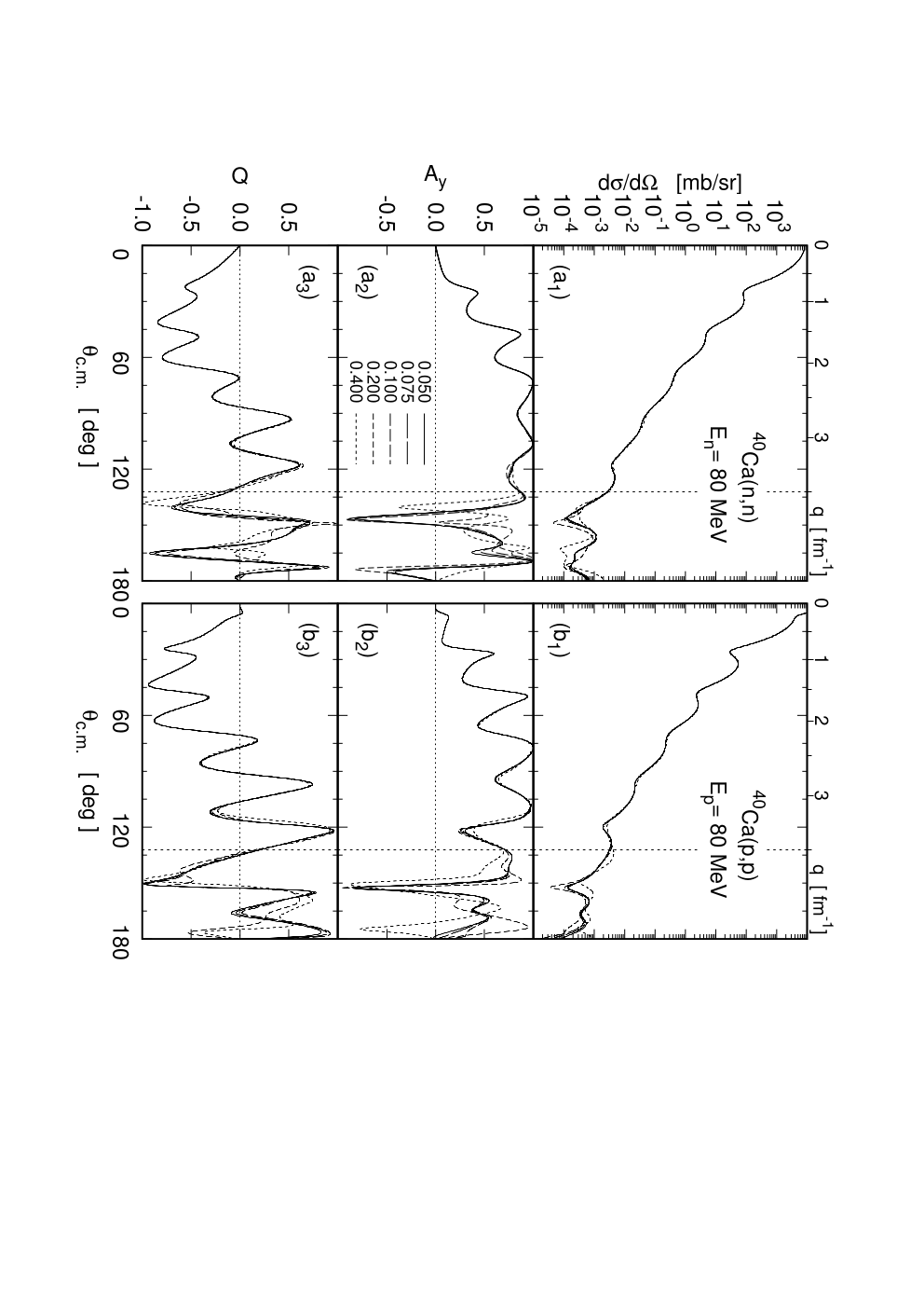
Along the same line as in the preceding section, we now consider neutron and proton scattering off ⁴⁰Ca at 80 MeV. In this case the potential is defined in momentum space, evaluated at 28 angles generated from Gaussian quadrature. Radial integration is up to $R_{max}\!=\!13.2$ fm, under KPOT=5. Scattering calculations by SWANLOP were performed considering $h\!=\!0.050$ , $0.075$ , $0.100$ , $0.200$ and $0.400$ fm. In Fig. 5 we plot results for $d\sigma\!/\!d\Omega$ ( $a_{1},b_{1}$ ), $A_{y}$ ( $a_{2},b_{2}$ ) and $Q$ ( $a_{3},b_{3}$ ) as functions of the scattering angle $\theta_{c.m.}$ . The upper scale denotes momentum transfer $q$ , with the vertical dotted line at $q\!=\!3.5$ fm^-1 drawn for reference. As in the $30.3$ MeV applications, NA scattering observables calculated with $h\!\leq\!0.1$ fm become difficult to distinguish from one another, from which we infer that $h\!=\!0.1$ fm enables converged results. For $h\!>\!0.1$ fm, instead, observables at $q\!>\!3.5$ fm^-1 depart from the rest as dotted and short-dashed curves become distinguishable. Momentum transfers of about 4 fm^-1 is a typical upper limit of scrutiny for NA scattering at intermediate energies [51], i.e. nucleon beam energies from a few hundred MeV to about $1$ GeV.

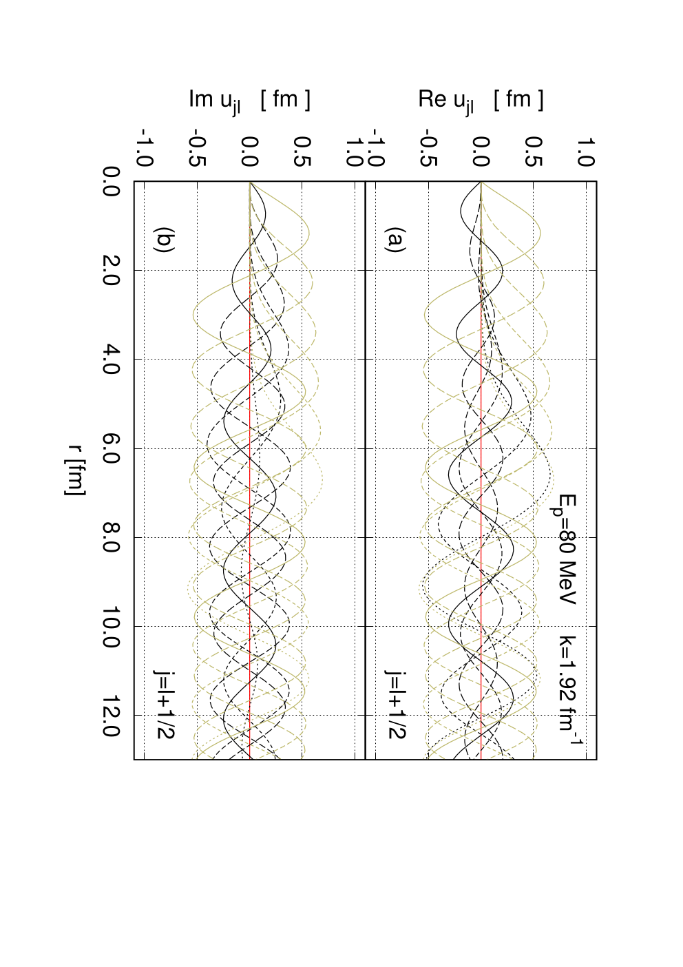
To complete this application at 80 MeV, in Fig. 6 we plot the scattering waves for ⁴⁰Ca( $p,p$ ), based on the same nonlocal potential calculated in momentum space. The beam momentum in this case is $k\!=\!1.92$ fm^-1, and select stretches states $j\!=\!l+\nicefrac{{1}}{{2}}$ , with $l\!\leq\!10$ . In panel (a) we show the real component of $u_{jl}$ whereas in panel (b) we plot its imaginary component. In these plots we consider waves with even $l$ , with $s$ waves plotted with solid lines. Waves with $l\!\geq\!2$ are plotted with segmented curves, with decreasing dash-length as $l$ increases. Colored curves represent undistorted incoming waves $F_{l}(kr)/k$ included here as reference in both panels. With this figure we intend to highlight the capability of SWANLOP to calculate scattering waves in collision described by momentum-space potentials, being this the first open code in doing so.

4.3 Comparison with SIDES

We now proceed to compare results for scattering observables obtained from SWANLOP and SIDES. As mentioned earlier, SIDES is a package developed to solve Schrödinger integro-differential equation in the presence of nonlocal potentials using finite differences techniques [37]. In the applications we pursue here we consider pA scattering with proton energies of 200 MeV, 700 MeV and 1 GeV. The targets to consider are ¹²C, ⁴⁰Ca, ⁹⁰Zr and ²⁰⁸Pb.

The nonlocal optical potentials for these processes are obtained from momentum-space calculations following Refs. [41, 52]. Specifically, applications at $200$ MeV are based on density-dependent $g$ -matrix folding model, with full account of the genuine $g$ matrix off shell. At $0.7$ and 1 GeV we use the off-shell $t\rho$ approximation. Relativistic kinematics in the calculation of the potential is included together with the account for hadronic absorption in the bare NN interaction above pion-production threshold [52]. The nonlocal one-body mixed densities are obtained within the Slater approximation [8] from local neutron and proton densities of the targets. These radial densities are obtained from self-consistent Hartree-Fock-Bogoliubov calculations with the Gogny force [53]. Once the momentum-space potential is calculated, SWANLOP generates its coordinate representation to be used by SIDES.

In Fig. 7 we plot —as functions of the momentum transfer $q$ — the differential cross section $d\sigma\!/\!d\Omega$ (upper row), analyzing power $A_{y}$ (middle row), and spin rotation function $Q$ (lower row), obtained from SWANLOP (solid curves) and SIDES (dashed curves). Columns (a), (b) and (c) correspond to proton energies $E_{p}$ of $200$ MeV, $700$ MeV and 1 GeV, respectively. To avoid superposition of curves in frames ( $a_{1}$ ), ( $b_{1}$ ) and ( $c_{1}$ ), results for $d\sigma\!/\!d\Omega$ in the cases of ²⁰⁸Pb and ⁹⁰Zr have been multiplied by $10$ , whereas those for ¹²C have been multiplied by $10^{-1}$ . Similarly, $A_{y}$ for ²⁰⁸Pb and ⁹⁰Zr have been up-shifted by $0.5$ , while those for ¹²C are down-shifted by the same amount ( $-0.5$ ). Identical considerations are made for $Q$ in the lower row.

As observed, the agreement between SWANLOP and SIDES results is quite satisfactory, where in most cases the curves from the two packages overlap each other. Some slight differences are observed for $Q$ at 200 MeV in the case of ¹²C( $p,p$ ) in panel ( $a_{3}$ ), around the minimum at $q\!\approx\!3$ fm^-1. This is despite the radical difference in the methods applied by the two packages, with SIDES using finite difference techniques to solve the integro-differential equation, while SWANLOP inverts $(1\!-\!\mathbb{K})$ in Eq. (20) to obtain the scattering wavefunction.

4.4 Performance

The actual time of execution of the code will depend upon the speed of the machine under use, in addition to the potential to be considered. However, we have found that the CPU run time $\tau$ with maximum angular momentum $L_{max}$ , using $N$ radial points can be estimated with

\tau=\tau_{0}\,(2L_{max}+1)\,N^{3}\;.

(47)

The base time $\tau_{0}$ depends on the machine. For a 2.6 GHz Intel® Core™ i7 processor used for all SWANLOP applications included in this work, we obtain $\tau_{0}\!=\!$11.5$$ ns. This is considering potentials in coordinate or momentum space read from file, suppressing print out of waves and potentials. With this, the run time for ²⁰⁸Pb( $p,p$ ) at 1 GeV using $N\!=\!320$ , and $L_{max}\!=\!129$ , would take $\tau\!=\!98$ s, while the actual run time is $97$ s. In the case of ¹²C at $200$ MeV with $N\!=\!110$ , and $L_{max}\!=31$ , Eq. (47) yields $\tau\!=\!1$ s, whereas the actual run time is 1.5 s. All TPM applications in Fig. 4 with $h\!=\!0.1$ fm take between 1 and 2 s. For PB-type potentials calculated internally, Eq. (47) for $\tau$ becomes inadequate above 50 MeV beam energy due to preponderance of time dedicated to multipole calculations.

We note that the total CPU run time $\tau$ depends on $L_{max}$ and $N$ , both quantities being guided by Eqs. (41), (42) and (43). In order to keep the focus on broad energy applications, with most targets in the nuclear chart, covering all scattering angles conditioned by maximum momentum transfer $q\!\sim\!4$ fm^-1, we have made no effort to optimize these quantities. Specific uses of the code, however, may allow to relax some of these parameters without compromising precision in observables of interest.

5 Summary and conclusions

We have introduced the self-contained package SWANLOP aimed to obtain accurate solutions for NA elastic scattering under nonlocal potentials for spin-zero target nuclei. The solution is theoretically motivated by Ref. [14], where scattering waves are obtained from a Lippmann-Schwinger type integral equation for the scattering waves. Its numerical implementation involves finite matrices over a spatial mesh, obtaining scattering waves by direct matrix inversion. Scattering observables such as differential cross sections $d\sigma\!/\!d\Omega$ , analyzing power $A_{y}$ and spin rotation function $Q$ , in addition to integrated cross sections are calculated. The code offers the possibility to treat local and nonlocal potentials, or admixture of both. Additionally, the code is capable of handling potentials in momentum space. This is an important feature since developments of microscopic or ab-initio models tend to evolve independently from different groups, mainly due to differences in the representation of their NA interactions. With the code SWANLOP it becomes possible, at least, to study scattering waves from those momentum-space potentials and compare them with those obtained in coordinate space.

Benchmark studies were carried out at nucleon energies from few MeV up to $1.1$ GeV, including light-, medium-mass and heavy targets, leading to consistent and reliable results. These tests also include comparison of results obtained from the code with those from analytic closed-form expression, where accuracy within $0.02$ % is obtained. We have also performed comparisons of angular scattering observables obtained from the package SIDES [37], at proton beam energies of $200$ , $700$ and $1000$ MeV, for light and heavy targets. Results from these applications show remarkable consistency between these two packages.

The calculation of scattering waves in NA collisions in the context of nonlocal potentials, superposed to the long-range Coulomb interaction, has been longstanding problem where specific solutions have been introduced under different assumptions on the nature of the nonlocality. These assumptions are either made explicit by their authors or made implicit in the adopted calculational scheme. In the case of momentum-space optical potentials, codes capable of obtaining their associated scattering waves have been non-existing. An important step forward has recently been achieved with the release of the package SIDES to solve Schrödinger’s integro-differential equation. With the introduction of SWANLOP package, we provide an alternative broad-use tool to obtain scattering waves —and associated observables— under any finite-range optical model potential, regardless of its representation in coordinate- or momentum-space, or features in its nonlocality.

Acknowledgments

H. F. A. is very grateful to colleagues of CEA,DAM,DIF for their kind hospitality during his stay at Bruyères-le-Châtel, where part of this collaboration took place. This research did not receive any specific grant from funding agencies in the public, commercial, or not-for-profit sectors.

Appendix A Relativistic corrections

Applications at high incident energies require the introduction of for relativistic effects. Corrections of kinematical origin are incorporated as follows. Let us consider a projectile of mass $m$ colliding a nucleus of mass $M$ at rest. The kinetic energy of the projectile in the laboratory reference frame is given by $E_{L}$ . Working in natural units $\hbar\!=\!c\!=\!1$ , the projectile-target relative momentum $k$ in the center-of-momentum reference frame is given by

k^{2}=\frac{1}{4s}\left[s-(m+M)^{2}\right]\left[s-(m-M)^{2}\right],

(48)

with the $s$ -invariant given by $s\!=\!2ME_{L}\!+\!(m\!+\!M)^{2}$ . Additionally, the reduced mass $\mu$ needs to be replaced by the reduced energy

\mu\to\frac{\varepsilon_{p}\,\varepsilon_{t}}{\varepsilon_{p}+\varepsilon_{t}}\,,

(49)

with $\varepsilon_{p}\!=\!\sqrt{k^{2}\!+\!m^{2}}$ , and $\varepsilon_{t}\!=\!\sqrt{k^{2}\!+\!M^{2}}$ . The kinetic energy in the center-of-momentum reference frame is given by $E\!=\!\varepsilon_{p}\!+\!\varepsilon_{t}\!-\!m\!-\!M$ . These corrections are obtained from Schrödinger’s wave equation written in the center-of-momentum reference frame,

\left(\sqrt{m^{2}+{\bm{p}}^{2}}+\sqrt{M^{2}+{\bm{p}}^{2}}+U\right)\Psi=(\varepsilon_{p}+\varepsilon_{t})\,\Psi\;,

(50)

followed by a first-order expansion of the square of the relative momentum operator ${\bm{p}}^{2}$ around $k^{2}$ .

Appendix B Coulomb potential

The potential energy between a charged projectile (proton) and the nucleus assumes a uniform proton density of radius $R_{{}_{C}}$ . Considering a target of charge $Ze$ , then the potential energy of the proton at a distance $r$ from the center of the nucleus is given by

V_{{}_{C}}(r)=\left\{\begin{array}[]{ll}\displaystyle{\frac{Ze^{2}}{2R_{{}_{C}}}\left[3-2\left(\frac{r}{R_{{}_{C}}}\right)^{2}\right]}&\qquad\textrm{for $r<R_{{}_{C}}$;}\\ &\\ \displaystyle{\frac{Ze^{2}}{r}}&\qquad\textrm{for $r\geq R_{{}_{C}}$.}\end{array}\right.

(51)

In the case of proton scattering using TPM parametrization of PB nonlocal model, we adopt $R_{{}_{C}}\!=$ $1.34$ fm. In all other cases we determine $R_{{}_{C}}$ using the extended liquid drop model of Ref. [54], where the charge root-mean-square radius is parametryzed as

\langle r^{2}\rangle_{ch}^{\nicefrac{{1}}{{2}}}=\sqrt{\textstyle{\frac{3}{5}}}\;A^{1/3}\left($1.15$+$1.80$\,A^{-2/3}-$1.20$\,A^{-4/3}\right)\;\textrm{fm}\;.

(52)

To the resulting charge mean-squared-radius (m.s.r), the proton charge m.s.r. $R_{p}^{\,2}$ is unfolded, with $R_{p}\!=\!$0.875$$ fm [42]. Therefore, the point-proton (pp) density m.s.r. becomes

\langle r^{2}\rangle_{pp}=\langle r^{2}\rangle_{ch}-R_{p}^{\,2}=\textstyle{\frac{3}{5}}\,R_{{}_{C}}^{\,2}\;.

(53)

From this expression we obtain $R_{{}_{C}}$ used by SWANLOP. In the package, subroutine vcoulomb.f can be customized by the user to adapt alternative forms to calculate $V_{{}_{C}}(r)$ .

Appendix C Integration entries and LMAX under potentials read from file

When a local potential is read from file then RMAX and NRP are taken from that file, while LMAX is defined by the user. In the case of PB nonlocal potentials (calculated internally by the code) the values of RMAX, NRP and LMAX are fully controlled by the user. However, if a nonlocal potential is read from file all the above entries are taken from that file. In the case of momentum-space potential read from file, LMAX is taken from the number of angular points over which the potential is defined, while both RMAX and NRP are defined by the user. All these considerations are summarized in Table 1, where checkmarks are placed on user-defined entries according to KPOT definition.

KPOT	RMAX	NRP	LMAX
0	–	–	✓
1	✓	✓	✓
2	✓	✓	✓
3	–	–	–
4	✓	✓	–

Table 1: Checkmarks on integration entries and LMAX to be specified by the user in main input file depending on the potential choice KPOT.

The code gives also the possibility of setting internally user-defined entries. To validate this action negative values must be supplied for the corresponding RMAX, NRP and/or LMAX. In that case Eqs. (41), (42) and (43) are used, keeping $h\!\leq\!0.1$ fm, with $R_{max}$ multiple of $0.5$ fm.

Appendix D Additional local potential option

Under setting KADD=1 or KADD=2 in line 11 of fort.1, a local potential is added to the potential defined under KPOT option. If KADD=1, the potential is read from fort.22 by subroutine read22.f, replacing any existing hadronic local term. If KADD=2, the additional local potential is calculated by user-customized subroutine user_vloc.f. In Table 2 we summarize actions taken by SWANLOP under KADD=0,1, depending on KPOT value.

KPOT	Action
0	Local term overwritten
1	PB local term overwritten
2	TPM local term overwritten
3	Local potential superposed
4	Local potential superposed

Table 2: Actions taken by SWANLOP under KADD=1 or 2, depending on KPOT entry.

Appendix E Analytic scattering matrix for separable potential

In the absence of Coulomb forces, for a given rank-1 separable potential $\hat{V}\!=\!|\xi\rangle\lambda\langle\xi|$ , the solution for the scattering matrix $\hat{T}(E)$ is given by

\hat{T}(E)=\frac{|\xi\rangle\lambda\langle\xi|}{1-\lambda\langle\xi|\hat{G}_{0}^{(+)}(E)\,|\xi\rangle}\;,

(54)

where $\hat{G}_{0}^{(+)}$ corresponds to the free propagator for outgoing waves. Projecting on-shell we get

\langle k|\hat{T}(E)|k\rangle=t(E)=\frac{\lambda\,|\tilde{\xi}(k)|^{2}}{1-\lambda\,\langle\xi|\hat{G}_{0}^{(+)}(E)\;|\xi\rangle}\;,

(55)

with $E\!=\!\hbar^{2}k^{2}/2\mu$ , and

\langle\xi|\hat{G}_{0}^{(+)}(E)\;|\xi\rangle=\frac{2}{\pi}\int_{0}^{\infty}\frac{p^{2}dp\,|\tilde{\xi}(p)|^{2}}{E+i\epsilon-\hbar^{2}p^{2}/2\mu}\;,

(56)

where $\epsilon$ is a positive infinitesimal to account for outgoing waves.

In the case of the separable potential in Ref. [50]

V(r^{\prime},r)=\lambda\,\xi_{n}(r^{\prime})\xi_{n}(r)\,,

(57)

the form factors are defined in coordinate space given as

\xi_{n}(r)=\exp(-\alpha r)(\alpha r)^{n}/r\;,

(58)

so that their corresponding form for $s$ waves in momentum representation becomes

\tilde{\xi}_{n}(p)=\langle p|\xi\rangle=\int_{0}^{\infty}r^{2}dr\,j_{0}(pr)\xi_{n}(r)\;.

(59)

With the use symbolic manipulation software Mathematica™ we obtain the explicit expressions


$\displaystyle\tilde{\xi}_{1}(p)$	$\displaystyle=\frac{2\alpha^{2}}{(\alpha^{2}+p^{2})^{2}};$	(60a)
$\displaystyle\tilde{\xi}_{2}(p)$	$\displaystyle=\frac{2\alpha^{2}(3\alpha^{2}-p^{2})}{(\alpha^{2}+p^{2})^{3}}.$	(60b)

We apply these results to evaluate $X_{n}(k)\!\equiv\!\langle\xi_{n}|\hat{G}_{0}^{(+)}(E)\;|\xi_{n}\rangle$ , in Eq. (56), obtaining the closed-form expressions


$\displaystyle X_{1}(x)$	$\displaystyle=-\frac{2\mu}{\hbar^{2}\alpha^{3}}\left[\frac{(5-15x^{2}-5x^{4}-x^{6})}{4(1+x^{2})^{4}}+i\frac{4x}{(1+x^{2})^{4}}\right]\;;$	(61a)
$\displaystyle X_{2}(x)$	$\displaystyle=-\frac{2\mu}{\hbar^{2}\alpha^{3}}\left[\frac{(11-2x^{2}+3x^{4})(3-19x^{2}-7x^{4}-x^{6})}{4(1+x^{2})^{6}}+i\frac{4x(3-x^{2})^{2}}{(1+x^{2})^{6}}\right]\,.$	(61b)

Thus, making use of Eqs. (60) and (61), the on-shell $T$ matrix in Eq. (55) becomes

t(E)=\frac{\lambda\;|\xi_{n}(k)|^{2}}{1-\lambda\;X_{n}(k)}\;,

(62)

where $k\!=\!\sqrt{2\mu E}$ . In these units the $S$ matrix is expressed by

S(E)=1-2i\,t(E)\;,

(63)

to be used in Eqs. (40) to evaluate cross sections.

In the case of form factors given by Eq. (46) we obtain simple closed forms for the volume integral per nucleon of the potential,

J/A=\frac{1}{A}\int d^{3}r_{1}\,d^{3}r_{2}U(r_{1},r_{2})=\frac{\lambda}{A}\left[\frac{4\pi(n+1)!}{\alpha^{2}}\right]^{2}\;,

(64)

and for the mean squared radius

\langle r^{2}\rangle=\frac{\int_{0}^{\infty}r^{4}\xi_{n}(r)dr}{\int_{0}^{\infty}r^{2}\xi_{n}(r)dr}=\frac{(n+2)(n+3)}{\alpha^{2}}\;.

(65)

These expressions become useful to calibrate values of $\alpha$ and $\lambda$ , from estimates of bulk size of the targets and $J/A$ values.

References

[1] J. Rotureau, P. Danielewicz, G. Hagen, F. M. Nunes, T. Papenbrock, Optical potential from first principles, Phys. Rev. C 95 (2017) 024315. doi:10.1103/PhysRevC.95.024315.
URL https://link.aps.org/doi/10.1103/PhysRevC.95.024315
[2] A. Idini, C. Barbieri, P. Navrátil, Ab initio optical potentials and nucleon scattering on medium mass nuclei, Phys. Rev. Lett. 123 (2019) 092501. doi:10.1103/PhysRevLett.123.092501.
URL https://link.aps.org/doi/10.1103/PhysRevLett.123.092501
[3] K. Mizuyama, K. Ogata, Self-consistent microscopic description of neutron scattering by ¹⁶o based on the continuum particle-vibration coupling method, Phys. Rev. C 86 (2012) 041603. doi:10.1103/PhysRevC.86.041603.
URL http://link.aps.org/doi/10.1103/PhysRevC.86.041603
[4] T. V. Nhan Hao, B. M. Loc, N. H. Phuc, Low-energy nucleon-nucleus scattering within the energy density functional approach, Phys. Rev. C 92 (2015) 014605. doi:10.1103/PhysRevC.92.014605.
URL http://link.aps.org/doi/10.1103/PhysRevC.92.014605
[5] G. Blanchon, M. Dupuis, H. F. Arellano, N. Vinh Mau, Microscopic positive-energy potential based on the Gogny interaction, Phys. Rev. C 91 (2015) 014612. doi:10.1103/PhysRevC.91.014612.
URL http://link.aps.org/doi/10.1103/PhysRevC.91.014612
[6] H. F. Arellano, F. A. Brieva, W. G. Love, In-medium full-folding optical model for nucleon-nucleus elastic scattering, Phys. Rev. C 52 (1995) 301–315. doi:10.1103/PhysRevC.52.301.
URL https://link.aps.org/doi/10.1103/PhysRevC.52.301
[7] M. Dupuis, S. Karataglidis, E. Bauge, J. P. Delaroche, D. Gogny, Correlations in microscopic optical model for nucleon elastic scattering off doubly closed-shell nuclei, Phys. Rev. C 73 (1) (2006) 014605. doi:10.1103/PhysRevC.73.014605.
[8] H. F. Arellano, F. A. Brieva, W. G. Love, Nonrelativistic full-folding model of nucleon elastic scattering at intermediate energies, Phys. Rev. C 41 (1990) 2188–2201. doi:10.1103/PhysRevC.41.2188.
[9] C. Elster, T. Cheon, E. F. Redish, P. C. Tandy, Full-folding optical potentials in elastic proton-nucleus scattering, Phys. Rev. C 41 (1990) 814–827. doi:10.1103/PhysRevC.41.814.
URL https://link.aps.org/doi/10.1103/PhysRevC.41.814
[10] R. Crespo, R. C. Johnson, J. A. Tostevin, Full folding calculations for proton-nucleus elastic scattering at intermediate energies, Phys. Rev. C 41 (1990) 2257–2262. doi:10.1103/PhysRevC.41.2257.
URL https://link.aps.org/doi/10.1103/PhysRevC.41.2257
[11] S. P. Weppner, C. Elster, D. Hüber, Off-shell structures of nucleon-nucleon $t$ matrices and their influence on nucleon-nucleus elastic scattering observables, Phys. Rev. C 57 (1998) 1378–1385. doi:10.1103/PhysRevC.57.1378.
URL https://link.aps.org/doi/10.1103/PhysRevC.57.1378
[12] M. Vorabbi, P. Finelli, C. Giusti, Theoretical optical potential derived from nucleon-nucleon chiral potentials, Phys. Rev. C 93 (2016) 034619. doi:10.1103/PhysRevC.93.034619.
[13] M. Burrows, C. Elster, S. P. Weppner, K. D. Launey, P. Maris, A. Nogga, G. Popa, Ab initio folding potentials for nucleon-nucleus scattering based on no-core shell-model one-body densities, Phys. Rev. C 99 (2019) 044603. doi:10.1103/PhysRevC.99.044603.
URL https://link.aps.org/doi/10.1103/PhysRevC.99.044603
[14] H. Arellano, G. Blanchon, Exact scattering waves off nonlocal potentials under Coulomb interaction within Schrödinger’s integro-differential equation, Physics Letters B 789 (2019) 256 – 261. doi:https://doi.org/10.1016/j.physletb.2018.12.004.
URL http://www.sciencedirect.com/science/article/pii/S0370269318309274
[15] F. Perey, B. Buck, A non-local potential model for the scattering of neutrons by nuclei, Nucl. Phys. 32 (1962) 353.
[16] L. J. Titus, F. M. Nunes, Testing the Perey effect, Phys. Rev. C 89 (2014) 034609. doi:10.1103/PhysRevC.89.034609.
URL https://link.aps.org/doi/10.1103/PhysRevC.89.034609
[17] L. Titus, A. Ross, F. Nunes, Transfer reaction code with nonlocal interactions, Computer Physics Communications 207 (2016) 499 – 517. doi:https://doi.org/10.1016/j.cpc.2016.06.022.
URL http://www.sciencedirect.com/science/article/pii/S0010465516302028
[18] N. J. Upadhyay, A. Bhagwat, B. K. Jain, A new treatment of nonlocality in scattering process, Journal of Physics G: Nuclear and Particle Physics 45 (1) (2018) 015106.
URL http://stacks.iop.org/0954-3899/45/i=1/a=015106
[19] N. J. Upadhyay, A. Bhagwat, Taylor approximation to treat nonlocality in the scattering process, Phys. Rev. C 98 (2018) 024605. doi:10.1103/PhysRevC.98.024605.
URL https://link.aps.org/doi/10.1103/PhysRevC.98.024605
[20] H. F. Arellano, G. Blanchon, Irreducible nonlocality of optical model potentials based on realistic nn interactions, Phys. Rev. C 98 (2018) 054616. doi:10.1103/PhysRevC.98.054616.
URL https://link.aps.org/doi/10.1103/PhysRevC.98.054616
[21] A. Picklesimer, P. C. Tandy, R. M. Thaler, D. H. Wolfe, Momentum space approach to microscopic effects in elastic proton scattering, Phys. Rev. C 30 (1984) 1861–1879. doi:10.1103/PhysRevC.30.1861.
URL https://link.aps.org/doi/10.1103/PhysRevC.30.1861
[22] C. R. Chinn, C. Elster, R. M. Thaler, Momentum-space treatment of Coulomb distortions in a multiple-scattering expansion, Phys. Rev. C 44 (1991) 1569–1580. doi:10.1103/PhysRevC.44.1569.
URL https://link.aps.org/doi/10.1103/PhysRevC.44.1569
[23] D. H. Lu, T. Mefford, R. H. Landau, G. Song, Coulomb plus nuclear scattering in momentum space for coupled angular momentum states, Phys. Rev. C 50 (1994) 3037–3046. doi:10.1103/PhysRevC.50.3037.
URL https://link.aps.org/doi/10.1103/PhysRevC.50.3037
[24] N. J. Upadhyay, V. Eremenko, L. Hlophe, F. M. Nunes, C. Elster, G. Arbanas, J. E. Escher, I. J. Thompson, Coulomb problem in momentum space without screening, Phys. Rev. C 90 (2014) 014615. doi:10.1103/PhysRevC.90.014615.
URL https://link.aps.org/doi/10.1103/PhysRevC.90.014615
[25] C. M. Vincent, S. C. Phatak, Accurate momentum-space method for scattering by nuclear and Coulomb potentials, Phys. Rev. C 10 (1974) 391–394. doi:10.1103/PhysRevC.10.391.
URL https://link.aps.org/doi/10.1103/PhysRevC.10.391
[26] R. A. Eisenstein, F. Tabakin, Nuclear densities in momentum space, Phys. Rev. C 26 (1982) 1–7. doi:10.1103/PhysRevC.26.1.
URL https://link.aps.org/doi/10.1103/PhysRevC.26.1
[27] E. O. Alt, W. Sandhas, H. Ziegelmann, Coulomb effects in three-body reactions with two charged particles, Phys. Rev. C 17 (1978) 1981–2005. doi:10.1103/PhysRevC.17.1981.
URL https://link.aps.org/doi/10.1103/PhysRevC.17.1981
[28] E. O. Alt, W. Sandhas, Scattering amplitudes and integral equations for the collision of two charged composite particles, Phys. Rev. C 21 (1980) 1733–1745. doi:10.1103/PhysRevC.21.1733.
URL https://link.aps.org/doi/10.1103/PhysRevC.21.1733
[29] A. Deltuva, A. C. Fonseca, P. U. Sauer, Momentum-space treatment of the Coulomb interaction in three-nucleon reactions with two protons, Phys. Rev. C 71 (2005) 054005. doi:10.1103/PhysRevC.71.054005.
URL https://link.aps.org/doi/10.1103/PhysRevC.71.054005
[30] A. Deltuva, A. C. Fonseca, P. U. Sauer, Momentum-space description of three-nucleon breakup reactions including the Coulomb interaction, Phys. Rev. C 72 (2005) 054004. doi:10.1103/PhysRevC.72.054004.
URL https://link.aps.org/doi/10.1103/PhysRevC.72.054004
[31] C. Elster, L. C. Liu, R. M. Thaler, Tech. Rep. LA-UR-90-2126, Los Alamos National Laboratory (1990).
[32] C. Elster, L. C. Liu, R. M. Thaler, A practical calculational method for treating Coulomb scattering in momentum space, Journal of Physics G: Nuclear and Particle Physics 19 (12) (1993) 2123–2134. doi:http://dx.doi.org/10.1088/0954-3899/19/12/015.
[33] B. T. Kim, T. Udagawa, Method for nonlocal optical model calculations, Phys. Rev. C 42 (1990) 1147–1149. doi:10.1103/PhysRevC.42.1147.
URL https://link.aps.org/doi/10.1103/PhysRevC.42.1147
[34] B. Kim, M. Kyum, S. Hong, M. Park, T. Udagawa, NLOM – a program for nonlocal optical model calculations, Computer Physics Communications 71 (1) (1992) 150 – 158. doi:https://doi.org/10.1016/0010-4655(92)90080-I.
URL http://www.sciencedirect.com/science/article/pii/001046559290080I
[35] G. Hagen, N. Michel, Elastic proton scattering of medium mass nuclei from coupled-cluster theory, Phys. Rev. C 86 (2012) 021602. doi:10.1103/PhysRevC.86.021602.
URL https://link.aps.org/doi/10.1103/PhysRevC.86.021602
[36] N. Michel, Numerical treatment of the long-range Coulomb potential with Berggren bases, Phys. Rev. C 83 (2011) 034325. doi:10.1103/PhysRevC.83.034325.
URL https://link.aps.org/doi/10.1103/PhysRevC.83.034325
[37] G. Blanchon, M. Dupuis, H. F. Arellano, R. N. Bernard, B. Morillon, Sides: Nucleon–nucleus elastic scattering code for nonlocal potential, Computer Physics Communications 254 (2020) 107340. doi:https://doi.org/10.1016/j.cpc.2020.107340.
URL http://www.sciencedirect.com/science/article/pii/S0010465520301478
[38] J. Raynal, Computer code dwba98, Tech. Rep. 1209/05, NEA (1998).
[39] W. R. Gibbs, Computation in Modern Physics, World Scientific Pub. Co. Inc., Singapore, 2006.
[40] M. Abramowitz, I. A. Stegun, Handbook of Mathematical Functions, Dover Poblications, 1965.
[41] F. J. Aguayo, H. F. Arellano, Surface-peaked medium effects in the interaction of nucleons with finite nuclei, Phys. Rev. C 78 (2008) 014608. doi:10.1103/PhysRevC.78.014608.
[42] M. Tanabashi, K. Hagiwara, K. Hikasa, K. Nakamura, Y. Sumino, F. Takahashi, J. Tanaka, K. Agashe, G. Aielli, C. Amsler, M. Antonelli, D. M. Asner, H. Baer, S. Banerjee, R. M. Barnett, T. Basaglia, C. W. Bauer, J. J. Beatty, V. I. Belousov, J. Beringer, S. Bethke, A. Bettini, H. Bichsel, O. Biebel, K. M. Black, E. Blucher, O. Buchmuller, V. Burkert, M. A. Bychkov, R. N. Cahn, M. Carena, A. Ceccucci, A. Cerri, D. Chakraborty, M.-C. Chen, R. S. Chivukula, G. Cowan, O. Dahl, G. D’Ambrosio, T. Damour, D. de Florian, A. de Gouvêa, T. DeGrand, P. de Jong, G. Dissertori, B. A. Dobrescu, M. D’Onofrio, M. Doser, M. Drees, H. K. Dreiner, D. A. Dwyer, P. Eerola, S. Eidelman, J. Ellis, J. Erler, V. V. Ezhela, W. Fetscher, B. D. Fields, R. Firestone, B. Foster, A. Freitas, H. Gallagher, L. Garren, H.-J. Gerber, G. Gerbier, T. Gershon, Y. Gershtein, T. Gherghetta, A. A. Godizov, M. Goodman, C. Grab, A. V. Gritsan, C. Grojean, D. E. Groom, M. Grünewald, A. Gurtu, T. Gutsche, H. E. Haber, C. Hanhart, S. Hashimoto, Y. Hayato, K. G. Hayes, A. Hebecker, S. Heinemeyer, B. Heltsley, J. J. Hernández-Rey, J. Hisano, A. Höcker, J. Holder, A. Holtkamp, T. Hyodo, K. D. Irwin, K. F. Johnson, M. Kado, M. Karliner, U. F. Katz, S. R. Klein, E. Klempt, R. V. Kowalewski, F. Krauss, M. Kreps, B. Krusche, Y. V. Kuyanov, Y. Kwon, O. Lahav, J. Laiho, J. Lesgourgues, A. Liddle, Z. Ligeti, C.-J. Lin, C. Lippmann, T. M. Liss, L. Littenberg, K. S. Lugovsky, S. B. Lugovsky, A. Lusiani, Y. Makida, F. Maltoni, T. Mannel, A. V. Manohar, W. J. Marciano, A. D. Martin, A. Masoni, J. Matthews, U.-G. Meißner, D. Milstead, R. E. Mitchell, K. Mönig, P. Molaro, F. Moortgat, M. Moskovic, H. Murayama, M. Narain, P. Nason, S. Navas, M. Neubert, P. Nevski, Y. Nir, K. A. Olive, S. Pagan Griso, J. Parsons, C. Patrignani, J. A. Peacock, M. Pennington, S. T. Petcov, V. A. Petrov, E. Pianori, A. Piepke, A. Pomarol, A. Quadt, J. Rademacker, G. Raffelt, B. N. Ratcliff, P. Richardson, A. Ringwald, S. Roesler, S. Rolli, A. Romaniouk, L. J. Rosenberg, J. L. Rosner, G. Rybka, R. A. Ryutin, C. T. Sachrajda, Y. Sakai, G. P. Salam, S. Sarkar, F. Sauli, O. Schneider, K. Scholberg, A. J. Schwartz, D. Scott, V. Sharma, S. R. Sharpe, T. Shutt, M. Silari, T. Sjöstrand, P. Skands, T. Skwarnicki, J. G. Smith, G. F. Smoot, S. Spanier, H. Spieler, C. Spiering, A. Stahl, S. L. Stone, T. Sumiyoshi, M. J. Syphers, K. Terashi, J. Terning, U. Thoma, R. S. Thorne, L. Tiator, M. Titov, N. P. Tkachenko, N. A. Törnqvist, D. R. Tovey, G. Valencia, R. Van de Water, N. Varelas, G. Venanzoni, L. Verde, M. G. Vincter, P. Vogel, A. Vogt, S. P. Wakely, W. Walkowiak, C. W. Walter, D. Wands, D. R. Ward, M. O. Wascko, G. Weiglein, D. H. Weinberg, E. J. Weinberg, M. White, L. R. Wiencke, S. Willocq, C. G. Wohl, J. Womersley, C. L. Woody, R. L. Workman, W.-M. Yao, G. P. Zeller, O. V. Zenin, R.-Y. Zhu, S.-L. Zhu, F. Zimmermann, P. A. Zyla, J. Anderson, L. Fuller, V. S. Lugovsky, P. Schaffner, Review of particle physics, Phys. Rev. D 98 (2018) 030001. doi:10.1103/PhysRevD.98.030001.
URL https://link.aps.org/doi/10.1103/PhysRevD.98.030001
[43] W. Huang, G. Audi, M. Wang, F. G. Kondev, S. Naimi, X. Xu, The ame2016 atomic mass evaluation (i). evaluation of input data and adjustment procedures, Chinese Physics C 41 (3) (2017) 030002. doi:10.1088/1674-1137/41/3/030002.
[44] M. Wang, G. Audi, F. G. Kondev, W. Huang, S. Naimi, X. Xu, The AME2016 atomic mass evaluation (II). Tables, graphs and references, Chinese Physics C 41 (3) (2017) 030003. doi:10.1088/1674-1137/41/3/030003.
[45] Y. Tian, D.-Y. Pang, Z.-Y. Ma, Systematic nonlocal optical model potential for nucleons, International Journal of Modern Physics E 24 (01) (2015) 1550006. doi:10.1142/S0218301315500068.
URL https://www.worldscientific.com/doi/abs/10.1142/S0218301315500068
[46] G. K. et. al, Halo structure of 8B determined from intermediate energy proton elastic scattering in inverse kinematics, Physics Letters B 780 (2018) 200 – 204. doi:https://doi.org/10.1016/j.physletb.2018.03.013.
URL http://www.sciencedirect.com/science/article/pii/S0370269318302016
[47] A. R. Barnett, COULFG: Coulomb and Bessel functions and their derivatives, for real arguments, by Steed’s method, Computer Physics Communications 27 (1982) 147–166.
URL http://www.sciencedirect.com/science/article/pii/0010465582900704
[48] J.-P. Moreau, Jean-Pierre Moreau’s Home Page, http://jean-pierre.moreau.pagesperso-orange.fr/Fortran/tseval_f90.txt (2020).
[49] G. E. Forsythe, M. A. Malcolm, C. B. Moler, Computer Methods for Mathematical Computations, Prentice-Hall, New Jersey, 1977.
[50] B. Bagchi, B. Mulligan, Analytic solutions in configuration space representation for scattering from a class of separable nonlocal potentials, Phys. Rev. C 10 (1974) 126–135. doi:10.1103/PhysRevC.10.126.
URL https://link.aps.org/doi/10.1103/PhysRevC.10.126
[51] W. C. L. Ray, G.W. Hoffmann, Nonrelativistic and relativistic descriptions of proton-nucleus scattering, Physics Reports 212 (1992) 223. doi:https://doi.org/10.1016/0370-1573(92)90156-T.
URL http://www.sciencedirect.com/science/article/pii/037015739290156T
[52] H. F. Arellano, H. V. von Geramb, Extension of the full-folding optical model for nucleon-nucleus scattering with applications up to 1.5 gev, Phys. Rev. C 66 (2002) 024602. doi:10.1103/PhysRevC.66.024602.
URL https://link.aps.org/doi/10.1103/PhysRevC.66.024602
[53] J. Dechargé, D. Gogny, Hartree-Fock-Bogolyubov calculations with the $D1$ effective interaction on spherical nuclei, Phys. Rev. C 21 (1980) 1568–1593. doi:10.1103/PhysRevC.21.1568.
URL https://link.aps.org/doi/10.1103/PhysRevC.21.1568
[54] W. D. Myers, K.-H. Schmidt, An update on droplet-model charge distributions, Nuclear Physics A 410 (1983) 61–73. doi:https://doi.org/10.1016/0375-9474(83)90401-3.
URL http://www.sciencedirect.com/science/article/pii/0375947483904013

l	r	Re $u_{-}$	Im $u_{-}$	Re $u_{+}$	Im $u_{+}$	$\textstyle{\frac{1}{k}}F_{l}(\eta,r)$
$\vdots$	$\vdots$	$\vdots$	$\vdots$	$\vdots$	$\vdots$	$\vdots$

SWANLOP : Scattering waves off nonlocal optical potentials in the presence of Coulomb interactionsJournal: Computer Physics Communications

Abstract

Keywords:

1 Introduction

2 Framework

2.1 Potential in momentum space

2.2 Elastic scattering observables

2.3 General considerations

3 The package SWANLOP

3.1 Data

3.2 Execution

3.3 Input files

3.3.1 Main input

3.3.2 KPOT option

3.3.3 Additional local potential

3.3.4 Chi-square evaluation

3.4 Output files

3.5 Credits

4 Benchmarks

4.1 Comparison against separable analytic solution

4.2 Convergence under step size for nonlocal optical-model potentials

4.2.1 TPM nonlocal model for pA scattering at 30.330.3 MeV

4.2.2 Momentum-space potential for nucleon scattering off 40Ca at 80 MeV

4.3 Comparison with SIDES

4.4 Performance

5 Summary and conclusions

Acknowledgments

Appendix A Relativistic corrections

Appendix B Coulomb potential

Appendix C Integration entries and LMAX under potentials read from file

Appendix D Additional local potential option

Appendix E Analytic scattering matrix for separable potential

References

References

4.2.1 TPM nonlocal model for pA scattering at $30.3$ MeV

4.2.2 Momentum-space potential for nucleon scattering off ⁴⁰Ca at 80 MeV