Bounding the finite-size error of quantum many-body dynamics simulations
Abstract
Finite-size error (FSE), the discrepancy between an observable in a finite system and in the thermodynamic limit, is ubiquitous in numerical simulations of quantum many body systems. Although a rough estimate of these errors can be obtained from a sequence of finite-size results, a strict, quantitative bound on the magnitude of FSE is still missing. Here we derive rigorous upper bounds on the FSE of local observables in real time quantum dynamics simulations initialized from a product state. In -dimensional locally interacting systems with a finite local Hilbert space, our bound implies , with , , , constants independent of and , which we compute explicitly. For periodic boundary conditions (PBC), the constant is twice as large as that for open boundary conditions (OBC), suggesting that PBC have smaller FSE than OBC at early times. The bound can be generalized to a large class of correlated initial states as well. As a byproduct, we prove that the FSE of local observables in ground state simulations decays exponentially with , under a suitable spectral gap condition. Our bounds are practically useful in determining the validity of finite-size results, as we demonstrate in simulations of the one-dimensional (1D) quantum Ising and Fermi-Hubbard models.
Introduction
Numerical simulations are crucial to our understanding of many-body quantum matter, and are routinely applied in all fields of physics and in chemistry. Unfortunately, many numerical techniques popular in these fields incur significant FSEs when approximating properties of a large (potentially infinite) system by properties of a finite one. The most direct example is exact diagonalization (ED), which exactly solves the finite system numerically Laflorencie and Poiblanc 2004; Noack and Manmana 2005; Sandvik 2010a; Läuchli 2011. Accessible system sizes are limited since the Hilbert space dimension grows exponentially with system size; for the simplest case of interacting spin-1/2s, a state-of-the-art ground state calculation is limited to spins 11 1 Reaching even these system sizes is possible only if internal, translation, and point group symmetries are utilized, and if state-of-the-art algorithms and large-scale computational resources are employed. Researchers usually employ much smaller systems for computational convenience.. FSEs also significantly affect other techniques, such as density matrix renormalization group (DMRG) White 1992; Hallberg 2006; Schollwöck 2011; Stoudenmire and White 2012, many tensor network algorithms Perez-Garcia et al. 2007; Orús 2014, quantum dynamical typicality-based algorithms Bartsch and Gemmer 2009; Elsayed and Fine 2013; Steinigeweg et al. 2014a; Steinigeweg et al. 2014b; Steinigeweg et al. 2014c, and quantum Monte Carlo (QMC) Nightingale and Umrigar 1999, and they are a significant source of error for simulating quantum systems on quantum computers Childs et al. 2018 and for analog quantum simulations using ultracold matter Bloch et al. 2012, trapped ions Blatt and Roos 2012, and other platforms Altman et al. 2019.
It is often difficult to characterize FSEs. The standard method to assess them is to calculate and compare observables for different system sizes, ideally using finite-size scaling Sandvik 2010b. Although useful, this method has limitations. One is that it offers no guarantees. Two different system sizes may have results that closely agree, but at larger sizes the physics changes and observables deviate Bausch et al. 2018. Another is that one may not be able to study multiple system sizes that are sufficiently large to get a good estimate of the convergence.
In this paper, we derive rigorous upper bounds on the error of approximating observables in a large, possibly infinite, quantum many-body system by results in a smaller one. The bounds are applicable to arbitrary Hamiltonians for which a Lieb-Robinson (LR) bound exists. For quantum dynamics simulations starting from product initial states and evolving under locally interacting Hamiltonians with a finite local Hilbert space, the bound for a local observable is
| (1) |
where , , , and are constants that can be computed explicitly and depend on the Hamiltonian, observable, and boundary condition. Such dynamics is explored in a wide variety of ultracold matter experiments, such as quantum quenches and slow ramps in Rydberg atoms Zeiher et al. 2016; Takei et al. 2016; Bernien et al. 2017; Guardado-Sanchez et al. 2018a; Lienhard et al. 2018; Orioli et al. 2018, molecules Yan et al. 2013; Hazzard et al. 2014; Seeßelberg et al. 2018, Fermi gases Smale et al. 2019, atoms in optical lattices de Paz et al. 2013; Meldgin et al. 2016; Choi et al. 2016; Bordia et al. 2017; Gabardos et al. 2020, and optical clocks Goban et al. 2018. This dynamics can probe fundamental phenomena, such as many-body localization Eisert et al. 2015; Nandkishore and Huse 2015; Luitz et al. 2016; Luitz and Lev 2017; Parameswaran and Vasseur 2018, prethermalization Mori et al. 2018; Schmied et al., and generation of topological defects near critical points Simon et al. 2011a. This bound is then extended to a large family of correlated initial states satisfying an exponential clustering condition. While our main focus is on dynamics, we also show that the FSE of local observables in a many-body ground state decays exponentially in system size, under a suitable spectral gap condition.
The idea behind our bound is that locality – specifically that one piece of a system does not instantly affect far-away pieces – imposes strong constraints on quantum dynamics Bravyi et al. 2006; Hastings 2010. This can be seen by considering evolution under a Hamiltonian initiated from a product state (other scenarios can be understood by similar arguments). As illustrated in Fig. 1, an observable in a region will be affected by FSEs only after a long enough time for information to propagate from the boundary to . This idea is made precise by relating FSE to unequal time correlation functions, which can then be bounded by a LR bound Lieb and Robinson 1972, a direct consequence of locality. Although similar ideas of applying LR bounds to analyze the performance of some numerical algorithms have been employed in Refs. Osborne 2006; Osborne 2007a; Osborne 2007b; Kliesch et al. 2014a; Woods et al. 2015; Woods and Plenio 2016; Haah et al. 2018; Tran et al. 2019; Huang 2020, the connection to FSE has not been made explicit, and the practical utility of the bounds for numerics was not demonstrated. This idea has also been applied to estimate FSE in a non-rigorous way, for example in Ref. Dağ and Sun 2020.
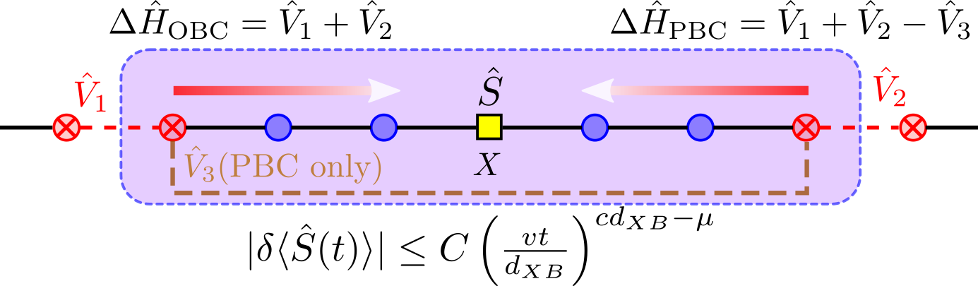
Our FSE bound not only shows the convergence of finite-size approximations in principle, but is tight enough to be useful in practice, which we demonstrate in simulations of some prototypical models. For example, in the dynamics following a sudden change of parameters in a 1D transverse field Ising model (TFIM) with sites, the error bounds for the transverse magnetization and nearest-neighbor correlations remain extremely small to times where they have evolved close to equilibrium. Furthermore, the bounds are reasonably tight: the time at which the error bound becomes significant is only 20–25% smaller than the time at which the actual FSE becomes noticeable. We similarly demonstrate this for the non-equilibrium relaxation of the Fermi-Hubbard model (FHM) from a checkerboard state, inspired by experiments and theory of Refs. Trotzky et al. 2012; Bauer et al. 2015. The precision of these bounds is enabled by the major quantitative improvements offered by recent LR bounds Chen and Lucas 2019a; Wang and Hazzard 2020.
In addition to their quantitative utility, these bounds provide insights into the convergence of numerical methods, and open the way to designing new algorithms. One immediate consequence of the bounds is to rigorously show that the FSE decays exponentially with the linear dimension of the system for periodic boundary condition (PBC), as well as for open boundary condition (OBC) provided that one measures observables only near the center of the system, as commonly employed in the DMRG community. If one instead averages the measurement over all sites in OBC, then our bound indicates that the error decays only algebraically. Similar behavior at finite temperature has been observed and analyzed in Ref. Iyer et al. 2015. Furthermore, if one compares PBC to OBC with center site measurement, our error bound for PBC decays twice as fast with distance as the bound for OBC at early times, suggesting that PBC gives more reliable results at early times 22 2 While the fact that the error bound for PBC is smaller than that for OBC does not necessarily imply that the actual FSE in PBC is smaller, in the Supplemental Material Sup we use short-time perturbative arguments to show that the actual error in PBC is indeed smaller at early times for most initial product states.. These insights may lead to new methods; one example is that they show why the moving-average cluster expansion (MACE) method of Ref. Hazzard et al. 2014 converges exponentially faster than alternative schemes.
A simple bound for both OBC and PBC
Consider the dynamical evolution of a quantum many-body system on an infinite -dimensional lattice, governed by a locally interacting Hamiltonian . For illustrative purpose, in Fig. 1 we draw the configuration for a 1D nearest-neighbor interacting lattice model. Let be the initial product state, be a local observable to be measured that acts on a finite region (center point in Fig. 1), and let be the sum of all the interaction terms between the inner and outer parts of the system (red links in Fig. 1). If PBC are used, we further subtract from the interaction between the first and the last site (brown link in Fig. 1). Let and denote the Hamiltonian and the initial state of the finite-size simulation, respectively (i.e. the restriction of and to the -site inner system). Denote , so that decouples into two commuting terms, one acting only on the inner system, the other acting only on the outer system. The FSE of the observable is
| (2) |
where , and we set throughout. Since decouples into two independent spatial regions (inner and outer) and is a product state, the first term in Eq. (2) can be rewritten as . Inserted into Eq. (2), the two expectation values are taken in the same state , so their difference can be bounded by the operator norm . Using the unitary invariance of operator norm for arbitrary unitary operators , we have
| (3) |
where is the evolution operator in the interaction picture, which satisfies and , where . Now applying the fundamental theorem of calculus and the triangle inequality, we obtain a bound on the FSE:
| (4) | |||||
The integrand is the quantity bounded by LR bounds, so to upper bound the FSE, one can insert the relevant LR bound. We focus on locally interacting systems, but Eq. (4) applies equally to long-range interactions by substituting the corresponding LR bounds Hastings and Koma 2006; Richerme et al. 2014; Gong et al. 2014; Foss-Feig et al. 2015; Tran et al. 2019; Chen and Lucas 2019b; Kuwahara and Saito 2020; Tran et al. 2020 in those systems. For a locally-interacting system, the currently tightest LR bound is obtained by computing the series in Eq. (S19) of the Supplemental Material (SM) Sup, which is based on Refs. Chen and Lucas 2019a; Wang and Hazzard 2020, although this may not be efficiently computable in general. A slightly looser but efficiently computable method is discussed in Ref. Wang and Hazzard 2020, in which one solves a system of first order linear differential equations for a number of variables proportional to the system size. To see the qualitative features of the bound for large systems, we can insert the simple expression given in Eq. (3) of Ref. Wang and Hazzard 2020 into Eq. (4) to obtain
| (5) |
where are constants independent of and , is the distance between the operators in the commutativity graph (CG) as introduced in Ref. Wang and Hazzard 2020, and is the LR speed. The distance in the CG is related to the distance in real space by , where are (straightforwardly determined) constants, and is the distance between and in real space. Therefore the rhs of Eq. (5) is bounded by , where . Despite its simplicity, the -dependence of this bound generically agrees with the exact error to lowest order in in OBC Sup.
Besides its practical utility for bounding FSE in calculations, as demonstrated below, this result has qualitative implications. One is to rigorously support the common practice of measuring observables close to the center site in OBC numerics (e.g. in the DMRG community), rather than averaging over all sites. This minimizes the error bound, since the center size maximizes . This choice yields our main result in Eq. (1) for the OBC case. Our bound allows one to extend this. For example, in dimension greater than one, we can minimize FSE by choosing an optimal cluster shape that minimizes the rhs of Eq. (5), and run simulations on the optimal shape.
An improved bound for PBC
In the previous section we treated PBC in a way similar to OBC. But it turns out that the resulting bound in Eqs. (4) and (5) is qualitatively loose at small for PBC. The reason for this can be intuitively understood as follows. The two terms in the rhs of Eq. (2) can be expanded in . As we discuss in greater detail in the SM Sup, the FSE for actually is only contributed by terms in whose spatial span is larger than and terms in that wrap around the whole periodic system. The leading order of these terms is proportional to , where is the length of the shortest non-contractible loop on the PBC commutativity graph, which is roughly twice as large as the exponent in Eq. (5). The SM Sup extends methods developed in Refs. Chen and Lucas 2019a; Wang and Hazzard 2020 to derive a rigorous upper bound for that leads to this improved scaling. The main result is
| (6) |
where the constant is given in Eq. (S52), is the LR speed in the -th direction given in Eq. (S53), and is the size of the periodic system in the -th direction in commutativity graph. is related to the real space system size by for constant integers . We note that while this bound improves the small-time exponent of the PBC bound by a factor of compared to Eqs. (4) and (5), the timescale on which the bound exponentially grows is still approximately the same as Eq. (5). Besides its quantitative utility, Eq. (6) shows that in anisotropic systems where is different in each direction, one should choose in order to minimize the FSE.
FSE in non-degenerate gapped ground states
So far, we have been discussing FSEs of quantum dynamics simulations. We now derive a bound on FSE of local observables in non-degenerate ground states under a gap assumption. This result is interesting in its own right, and will also be useful for our subsequent generalization of the dynamics error bound to correlated initial states.
The Hamiltonian , observable , boundary terms , etc. are the same as before. For convenience we suppose that the operator has unit norm and acts nontrivially only within a region of diameter which sits on the center of the finite-size cluster. The difference now is that we consider the observable given by the ground state density matrix . The numerical simulation approximates this thermodynamic quantity by the expectation value in the finite size ground state , where is the ground state density matrix of . Our result relies on an assumption that the interpolated Hamiltonain is non-degenerate for all and has a uniform spectral gap . When this condition is satisfied, then analogously to Eq. (1) we have Sup
| (7) |
Bounds for correlated initial states
We now generalize our error bound to dynamics initiated from a class of (possibly mixed) initial states , for which there exists a sufficiently good finite size approximation satisfying Eq. (7). This includes non-degenerate gapped ground states (under the condition described above), but also includes translation invariant matrix product states (MPS) with a finite bond dimension 33 3 For translation invariant MPS with a finite bond dimension, can be taken as the -site periodic version of . That satisfies the condition in Eq. (7) can be proved using the transfer operator method which is used to prove that MPS has finite correlation length, see, e.g. Refs. Schollwöck 2011; Perez-Garcia et al. 2007; Orús 2014. The parameter can simply be taken as the correlation length of the MPS., and finite temperature thermal states Kliesch et al. 2014b above a certain temperature, where , i.e. the thermal state of .
Given that we have an initial state satisfying Eq. (7), we can bound the dynamics FSE as
| (8) | |||||
where , is the reduced density matrix of on the finite cluster, and in the second line we used the triangle inequality. The second term can be bounded using the same method as in Eq. (2), since for any density matrix . To bound the first term, we insert the expansion into Eq. (8), and notice that is an operator acting on , whose norm is bounded by Eqs. (4,5) to be for some constant . For initial states satisfying Eq. (7), this implies
| (9) |
where and are model-dependent constants that can be explicitly determined.
Example: 1D TFIM
We test our dynamics error bounds in simulations of prototypical models for quantum many-body physics, starting with the TFIM,
| (10) |
This is a canonical model for quantum phase transitions Vojta 2003; Sachdev 2007, and occurs in materials like CoNb2O6 Coldea et al. 2010, cold atom Simon et al. 2011b; Labuhn et al. 2016; Guardado-Sanchez et al. 2018b and trapped ion Friedenauer et al. 2008; Kim et al. 2010; Kim et al. 2011; Lanyon et al. 2011; Britton et al. 2012 experiments, and superconducting circuits Barends et al. 2016; Harris et al. 2018. We numerically study the dynamics of this model at the critical point for several , and calculate the exact evolution for . Specifically, we study the dynamics of starting from . Analogous dynamics in the 2D TFIM has been explored in Rydberg atom experiments Guardado-Sanchez et al. 2018a; Lienhard et al. 2018.
Fig. 2a shows from to using PBC, along with the exact solution Dziarmaga 2005. To obtain a FSE bound for , we use the LR bound given in Eq. (S24) of Ref. Sup [obtained from the general bound Eq. (S20)], which, after inserting into Eq. (4), yields
| (11) |
As Fig. 2a shows, this error bound provides a guarantee of the numerical calculations’ accuracy out to interesting and useful timescales. For the -site calculation, the bound guarantees that the results are accurate (within ) up to times , where the observable has nearly reached equilibrium. Furthermore, this time is in reasonable accord with the true time at which FSE becomes important (within 20%).
We emphasize that the FSE bound never made use of the TFIM’s exact solution. The bound Eq. (4) can be applied to any system including in dimensions greater than one. As we will now demonstrate in the 1D FHM, the bound still provides a useful guarantee of the finite-size results when no exact solution is available.

Example: FHM
The 1D FHM describes spin-1/2 fermions in a lattice whose Hamiltonian is
| (12) |
The FHM exhibits rich behavior, such as a metal-Mott insulator transition, and potentially high-temperature superconductivity. It is a reasonable approximation of some real materials, such as FeO, NiO, CoO Anisimov et al. 1991, and has been realized in ultracold atoms Esslinger 2010; Parsons et al. 2016; Boll et al. 2016; Mazurenko et al. 2017; Brown et al. 2019.
We numerically study the relaxation dynamics of a charge density wave state , analogous to previous theory Schlünzen et al. 2017 and experiments Pertot et al. 2014, where (0) means a doubly occupied (empty) site. We run the finite-size simulations in OBC, and measure the density imbalance Schlünzen et al. 2017. To get a FSE bound for , we use the currently tightest LR bound, obtained by numerically summing the series in Eq. (S19) of the SM Sup and inserting the result into Eq. (4). Fig. 2b shows the results.
Our error bound can be compared to estimates of FSE obtained from comparing calculations of different sizes. For example, one can take the difference between the and as a rough estimate of the FSE of the calculation. Our bound is comparable in its guaranteed timescale of convergence to this conventional estimate. For example, we can guarantee that the FSE in of the result is less than for , comparable to the time where the and results differ noticeably.
Conclusions
We have presented a rigorous upper bound on the FSE of local observables measured in numerical simulations of quantum dynamics starting from a large class of initial states. For product initial states, the bounds show an advantage of using PBC at early times. We also presented a generalization to simulations of local observables in non-degenerate gapped ground states. In all the cases we considered, the bounds decay exponentially in system size, and guarantee the accuracy of finite size dynamics simulation up to a time scale . These insights into FSE can motivate better algorithms.
The quantitative utility of the bounds is demonstrated in the 1D TFIM and 1D FHM. In both cases, the error bounds are extremely small up to timescales where there is interesting physics and even equilibration, and they are reasonably tight compared to the actual FSEs. We expect these bounds to provide useful tools to researchers going forward, providing FSE bounds on numerical calculations and suggesting new numerical methods that minimize this error.
Acknowledgements.
We thank Miles Stoudenmire, Miroslav Hopjan, Bhuvanesh Sundar and Ian White for discussions, and Brian Neyenhuis for a careful reading of the manuscript. This work was supported in part by the Welch Foundation (C-1872), the National Science Foundation (PHY-1848304), and the Office of Naval Research (N00014-20-1-2695).References
- Laflorencie and Poiblanc (2004) N. Laflorencie and D. Poiblanc, “Quantum magnetism. lecture notes in physics,” (Springer-Verlag, 2004) Chap. Simulations of pure and doped low-dimensional spin-1/2 gapped systems.
- Noack and Manmana (2005) R. M. Noack and S. R. Manmana, AIP Conf. Proc. 789, 93 (2005).
- Sandvik (2010a) A. W. Sandvik, AIP Conf. Proc. 1297, 135 (2010a).
- Läuchli (2011) A. Läuchli, “Introduction to frustrated magnetism: Materials, experiments, theory,” (Springer, 2011) Chap. Numerical Simulations of Frustrated Systems, pp. 481 – 511.
- (5) Reaching even these system sizes is possible only if internal, translation, and point group symmetries are utilized, and if state-of-the-art algorithms and large-scale computational resources are employed. Researchers usually employ much smaller systems for computational convenience.
- White (1992) S. R. White, Phys. Rev. Lett. 69, 2863 (1992).
- Hallberg (2006) K. A. Hallberg, Adv. Phys. 55, 477 (2006).
- Schollwöck (2011) U. Schollwöck, Ann. Phys. 326, 96 (2011).
- Stoudenmire and White (2012) E. M. Stoudenmire and S. R. White, Annu. Rev. Condens. Matter Phys. 3, 111 (2012).
- Perez-Garcia et al. (2007) D. Perez-Garcia, F. Verstraete, M. M. Wolf, and J. I. Cirac, Quantum Info. Comput. 7, 401–430 (2007).
- Orús (2014) R. Orús, Ann. Phys. 349, 117 (2014).
- Bartsch and Gemmer (2009) C. Bartsch and J. Gemmer, Phys. Rev. Lett. 102, 110403 (2009).
- Elsayed and Fine (2013) T. A. Elsayed and B. V. Fine, Phys. Rev. Lett. 110, 070404 (2013).
- Steinigeweg et al. (2014a) R. Steinigeweg, A. Khodja, H. Niemeyer, C. Gogolin, and J. Gemmer, Phys. Rev. Lett. 112, 130403 (2014a).
- Steinigeweg et al. (2014b) R. Steinigeweg, J. Gemmer, and W. Brenig, Phys. Rev. Lett. 112, 120601 (2014b).
- Steinigeweg et al. (2014c) R. Steinigeweg, F. Heidrich-Meisner, J. Gemmer, K. Michielsen, and H. De Raedt, Phys. Rev. B 90, 094417 (2014c).
- Nightingale and Umrigar (1999) M. P. Nightingale and C. J. Umrigar, eds., Quantum Monte Carlo Methods in Physics and Chemistry (Springer, 1999).
- Childs et al. (2018) A. M. Childs, D. Maslov, Y. Nam, N. J. Ross, and Y. Su, Proc. Natl. Acad. Sci. 115, 9456 (2018).
- Bloch et al. (2012) I. Bloch, J. Dalibard, and S. Nascimbène, Nat. Phys. 8, 267 (2012).
- Blatt and Roos (2012) R. Blatt and C. F. Roos, Nat. Phys. 8, 277 (2012).
- Altman et al. (2019) E. Altman, K. R. Brown, G. Carleo, L. D. Carr, E. Demler, C. Chin, B. DeMarco, S. E. Economou, M. A. Eriksson, K.-M. C. Fu, et al., arXiv:1912.06938 (2019).
- Sandvik (2010b) A. W. Sandvik, in AIP Conference Proceedings, Vol. 1297 (American Institute of Physics, 2010) pp. 135–338.
- Bausch et al. (2018) J. Bausch, T. S. Cubitt, A. Lucia, D. Perez-Garcia, and M. M. Wolf, Proc. Natl. Acad. Sci. U.S.A 115, 19 (2018).
- Zeiher et al. (2016) J. Zeiher, R. van Bijnen, P. Schauß, S. Hild, J.-Y. Choi, T. Pohl, I. Bloch, and C. Gross, Nat. Phys. 12, 1095 (2016).
- Takei et al. (2016) N. Takei, C. Sommer, C. Genes, G. Pupillo, H. Goto, K. Koyasu, H. Chiba, M. Weidemüller, and K. Ohmori, Nature Communications 7, 13449 (2016).
- Bernien et al. (2017) H. Bernien, S. Schwartz, A. Keesling, H. Levine, A. Omran, H. Pichler, S. Choi, A. S. Zibrov, M. Endres, M. Greiner, et al., Nature 551, 579 (2017).
- Guardado-Sanchez et al. (2018a) E. Guardado-Sanchez, P. T. Brown, D. Mitra, T. Devakul, D. A. Huse, P. Schauß, and W. S. Bakr, Phys. Rev. X 8, 021069 (2018a).
- Lienhard et al. (2018) V. Lienhard, S. de Léséleuc, D. Barredo, T. Lahaye, A. Browaeys, M. Schuler, L.-P. Henry, and A. M. Läuchli, Phys. Rev. X 8, 021070 (2018).
- Orioli et al. (2018) A. P. Orioli, A. Signoles, H. Wildhagen, G. Günter, J. Berges, S. Whitlock, and M. Weidemüller, Phys. Rev. Lett. 120, 063601 (2018).
- Yan et al. (2013) B. Yan, S. A. Moses, B. Gadway, J. P. Covey, K. R. A. Hazzard, A. M. Rey, D. S. Jin, and J. Ye, Nature 501, 521 (2013).
- Hazzard et al. (2014) K. R. A. Hazzard, B. Gadway, M. Foss-Feig, B. Yan, S. A. Moses, J. P. Covey, N. Y. Yao, M. D. Lukin, J. Ye, D. S. Jin, and A. M. Rey, Phys. Rev. Lett. 113, 195302 (2014).
- Seeßelberg et al. (2018) F. Seeßelberg, X.-Y. Luo, M. Li, R. Bause, S. Kotochigova, I. Bloch, and C. Gohle, Phys. Rev. Lett. 121, 253401 (2018).
- Smale et al. (2019) S. Smale, P. He, B. A. Olsen, K. G. Jackson, H. Sharum, S. Trotzky, J. Marino, A. M. Rey, and J. H. Thywissen, Sci. Adv. 5 (2019), 10.1126/sciadv.aax1568.
- de Paz et al. (2013) A. de Paz, A. Sharma, A. Chotia, E. Marechal, J. H. Huckans, P. Pedri, L. Santos, O. Gorceix, L. Vernac, and B. Laburthe-Tolra, Phys. Rev. Lett. 111, 185305 (2013).
- Meldgin et al. (2016) C. Meldgin, U. Ray, P. Russ, D. Chen, D. M. Ceperley, and B. DeMarco, Nat. Phys. 12, 646 (2016).
- Choi et al. (2016) J.-Y. Choi, S. Hild, J. Zeiher, P. Schauß, A. Rubio-Abadal, T. Yefsah, V. Khemani, D. A. Huse, I. Bloch, and C. Gross, Science 352, 1547 (2016).
- Bordia et al. (2017) P. Bordia, H. Lüschen, S. Scherg, S. Gopalakrishnan, M. Knap, U. Schneider, and I. Bloch, Phys. Rev. X 7, 041047 (2017).
- Gabardos et al. (2020) L. Gabardos, B. Zhu, S. Lepoutre, A. M. Rey, B. Laburthe-Tolra, and L. Vernac, arXiv:2005.13487 (2020).
- Goban et al. (2018) A. Goban, R. B. Hutson, G. E. Marti, S. L. Campbell, M. A. Perlin, P. S. Julienne, J. P. D’Incao, A. M. Rey, and J. Ye, Nature 563, 369 (2018).
- Eisert et al. (2015) J. Eisert, M. Friesdorf, and C. Gogolin, Nat. Phys. 11, 124 (2015).
- Nandkishore and Huse (2015) R. Nandkishore and D. A. Huse, Annu. Rev. Condens. Matter Phys. 6, 15 (2015).
- Luitz et al. (2016) D. J. Luitz, N. Laflorencie, and F. Alet, Phys. Rev. B 93, 060201(R) (2016).
- Luitz and Lev (2017) D. J. Luitz and Y. B. Lev, Ann. Phys. (Berlin) 529, 1600350 (2017).
- Parameswaran and Vasseur (2018) S. A. Parameswaran and R. Vasseur, Rep. Prog. Phys. 81, 082501 (2018).
- Mori et al. (2018) T. Mori, T. N. Ikeda, E. Kaminishi, and M. Ueda, J. Phys. B 51, 112001 (2018).
- (46) C.-M. Schmied, A. N. Mikheev, and T. Gasenzer, arXiv:1810.08143 .
- Simon et al. (2011a) J. Simon, W. S. Bakr, R. Ma, M. E. Tai, P. M. Preiss, and M. Greiner, Nature 472, 307 (2011a).
- Bravyi et al. (2006) S. Bravyi, M. B. Hastings, and F. Verstraete, Phys. Rev. Lett. 97, 050401 (2006).
- Hastings (2010) M. B. Hastings, arXiv:1008.5137 (2010).
- Lieb and Robinson (1972) E. H. Lieb and D. W. Robinson, Commun. Math. Phys. 28, 251 (1972).
- Osborne (2006) T. J. Osborne, Phys. Rev. Lett. 97, 157202 (2006).
- Osborne (2007a) T. J. Osborne, Phys. Rev. A 75, 032321 (2007a).
- Osborne (2007b) T. J. Osborne, Phys. Rev. A 75, 042306 (2007b).
- Kliesch et al. (2014a) M. Kliesch, C. Gogolin, and J. Eisert, in Many-Electron Approaches in Physics, Chemistry and Mathematics (Springer, 2014) pp. 301–318.
- Woods et al. (2015) M. P. Woods, M. Cramer, and M. B. Plenio, Phys. Rev. Lett. 115, 130401 (2015).
- Woods and Plenio (2016) M. P. Woods and M. B. Plenio, J. Math. Phys. 57, 022105 (2016).
- Haah et al. (2018) J. Haah, M. Hastings, R. Kothari, and G. H. Low, in 2018 IEEE 59th Annual Symposium on Foundations of Computer Science (FOCS) (IEEE, 2018) pp. 350–360.
- Tran et al. (2019) M. C. Tran, A. Y. Guo, Y. Su, J. R. Garrison, Z. Eldredge, M. Foss-Feig, A. M. Childs, and A. V. Gorshkov, Phys. Rev. X 9, 031006 (2019).
- Huang (2020) Y. Huang, arXiv:2001.10763 (2020).
- Dağ and Sun (2020) C. B. Dağ and K. Sun, arXiv preprint arXiv:2004.12287 (2020).
- Trotzky et al. (2012) S. Trotzky, Y.-A. Chen, A. Flesch, I. P. McCulloch, U. Schollwöck, J. Eisert, and I. Bloch, Nat. Phys. 8, 325 (2012).
- Bauer et al. (2015) A. Bauer, F. Dorfner, and F. Heidrich-Meisner, Phys. Rev. A 91, 053628 (2015).
- Chen and Lucas (2019a) C.-F. Chen and A. Lucas, arXiv preprint arXiv:1905.03682 (2019a).
- Wang and Hazzard (2020) Z. Wang and K. R. A. Hazzard, PRX Quantum 1, 010303 (2020).
- Iyer et al. (2015) D. Iyer, M. Srednicki, and M. Rigol, Phys. Rev. E 91, 062142 (2015).
- (66) While the fact that the error bound for PBC is smaller than that for OBC does not necessarily imply that the actual FSE in PBC is smaller, in the Supplemental Material Sup we use short-time perturbative arguments to show that the actual error in PBC is indeed smaller at early times for most initial product states.
- Hastings and Koma (2006) M. B. Hastings and T. Koma, Commun. Math. Phys. 265, 781 (2006).
- Richerme et al. (2014) P. Richerme, Z.-X. Gong, A. Lee, C. Senko, J. Smith, M. Foss-Feig, S. Michalakis, A. V. Gorshkov, and C. Monroe, Nature 511, 198 (2014).
- Gong et al. (2014) Z.-X. Gong, M. Foss-Feig, S. Michalakis, and A. V. Gorshkov, Phys. Rev. Lett. 113, 030602 (2014).
- Foss-Feig et al. (2015) M. Foss-Feig, Z.-X. Gong, C. W. Clark, and A. V. Gorshkov, Phys. Rev. Lett. 114, 157201 (2015).
- Chen and Lucas (2019b) C.-F. Chen and A. Lucas, Phys. Rev. Lett. 123, 250605 (2019b).
- Kuwahara and Saito (2020) T. Kuwahara and K. Saito, Phys. Rev. X 10, 031010 (2020).
- Tran et al. (2020) M. C. Tran, C.-F. Chen, A. Ehrenberg, A. Y. Guo, A. Deshpande, Y. Hong, Z.-X. Gong, A. V. Gorshkov, and A. Lucas, Phys. Rev. X 10, 031009 (2020).
- (74) See Supplemental Material for the comparison of the error bounds to perturbation theory at early times, the detailed derivation of the PBC error bound in Eq. (S18), the detailed proof of Eqs. (7) and (9), and detailed derivations and expressions for the three different methods to bound the rhs of Eq. (S18). The numerically tightest one is given in Eq. (S20), a more efficiently computable one is given in Eq. (S39), and the constants for the simplest one Eq. (6) are given in Eqs. (S52,S53,S55).
- (75) For translation invariant MPS with a finite bond dimension, can be taken as the -site periodic version of . That satisfies the condition in Eq. (7) can be proved using the transfer operator method which is used to prove that MPS has finite correlation length, see, e.g. Refs. Schollwöck 2011; Perez-Garcia et al. 2007; Orús 2014. The parameter can simply be taken as the correlation length of the MPS.
- Kliesch et al. (2014b) M. Kliesch, C. Gogolin, M. J. Kastoryano, A. Riera, and J. Eisert, Phys. Rev. X 4, 031019 (2014b).
- Vojta (2003) M. Vojta, Rep. Prog. Phys. 66, 2069 (2003).
- Sachdev (2007) S. Sachdev, “Quantum phase transitions,” in Handbook of Magnetism and Advanced Magnetic Materials (American Cancer Society, 2007) https://onlinelibrary.wiley.com/doi/pdf/10.1002/9780470022184.hmm108 .
- Coldea et al. (2010) R. Coldea, D. A. Tennant, E. M. Wheeler, E. Wawrzynska, D. Prabhakaran, M. Telling, K. Habicht, P. Smeibidl, and K. Kiefer, Science 327, 177 (2010).
- Simon et al. (2011b) J. Simon, W. S. Bakr, R. Ma, M. E. Tai, P. M. Preiss, and M. Greiner, Nature 472, 307 (2011b).
- Labuhn et al. (2016) H. Labuhn, D. Barredo, S. Ravets, S. De Léséleuc, T. Macrì, T. Lahaye, and A. Browaeys, Nature 534, 667 (2016).
- Guardado-Sanchez et al. (2018b) E. Guardado-Sanchez, P. T. Brown, D. Mitra, T. Devakul, D. A. Huse, P. Schauß, and W. S. Bakr, Phys. Rev. X 8, 021069 (2018b).
- Friedenauer et al. (2008) A. Friedenauer, H. Schmitz, J. T. Glueckert, D. Porras, and T. Schätz, Nat. Phys. 4, 757 (2008).
- Kim et al. (2010) K. Kim, M.-S. Chang, S. Korenblit, R. Islam, E. E. Edwards, J. K. Freericks, G.-D. Lin, L.-M. Duan, and C. Monroe, Nature 465, 590 (2010).
- Kim et al. (2011) K. Kim, S. Korenblit, R. Islam, E. Edwards, M. Chang, C. Noh, H. Carmichael, G. Lin, L. Duan, C. J. Wang, et al., New J. Phys. 13, 105003 (2011).
- Lanyon et al. (2011) B. P. Lanyon, C. Hempel, D. Nigg, M. Müller, R. Gerritsma, F. Zähringer, P. Schindler, J. T. Barreiro, M. Rambach, G. Kirchmair, et al., Science 334, 57 (2011).
- Britton et al. (2012) J. W. Britton, B. C. Sawyer, A. C. Keith, C.-C. J. Wang, J. K. Freericks, H. Uys, M. J. Biercuk, and J. J. Bollinger, Nature 484, 489 (2012).
- Barends et al. (2016) R. Barends, A. Shabani, L. Lamata, J. Kelly, A. Mezzacapo, U. Las Heras, R. Babbush, A. G. Fowler, B. Campbell, Y. Chen, et al., Nature 534, 222 (2016).
- Harris et al. (2018) R. Harris, Y. Sato, A. Berkley, M. Reis, F. Altomare, M. Amin, K. Boothby, P. Bunyk, C. Deng, C. Enderud, et al., Science 361, 162 (2018).
- Dziarmaga (2005) J. Dziarmaga, Phys. Rev. Lett. 95, 245701 (2005).
- Anisimov et al. (1991) V. I. Anisimov, J. Zaanen, and O. K. Andersen, Phys. Rev. B 44, 943 (1991).
- Esslinger (2010) T. Esslinger, Annu. Rev. Condens. Matter Phys. 1, 129 (2010).
- Parsons et al. (2016) M. F. Parsons, A. Mazurenko, C. S. Chiu, G. Ji, D. Greif, and M. Greiner, Science 353, 1253 (2016).
- Boll et al. (2016) M. Boll, T. A. Hilker, G. Salomon, A. Omran, J. Nespolo, L. Pollet, I. Bloch, and C. Gross, Science 353, 1257 (2016).
- Mazurenko et al. (2017) A. Mazurenko, C. S. Chiu, G. Ji, M. F. Parsons, M. Kanász-Nagy, R. Schmidt, F. Grusdt, E. Demler, D. Greif, and M. Greiner, Nature 545, 462 (2017).
- Brown et al. (2019) P. T. Brown, D. Mitra, E. Guardado-Sanchez, R. Nourafkan, A. Reymbaut, C.-D. Hébert, S. Bergeron, A.-M. Tremblay, J. Kokalj, D. A. Huse, et al., Science 363, 379 (2019).
- Schlünzen et al. (2017) N. Schlünzen, J.-P. Joost, F. Heidrich-Meisner, and M. Bonitz, Phys. Rev. B 95, 165139 (2017).
- Pertot et al. (2014) D. Pertot, A. Sheikhan, E. Cocchi, L. A. Miller, J. E. Bohn, M. Koschorreck, M. Köhl, and C. Kollath, Phys. Rev. Lett. 113, 170403 (2014).
- Schuch et al. (2011) N. Schuch, S. K. Harrison, T. J. Osborne, and J. Eisert, Phys. Rev. A 84, 032309 (2011).
Supplemental Material for
“Bounding the FSE of quantum many-body dynamics simulations”
Zhiyuan Wang, Michael Foss-Feig, and Kaden R. A. Hazzard
The supplemental material fills in technical details of the basic results in the main text. We first prove the ground state FSE bound in Eq. (7) under the gap assumption we mentioned there. Then we give the full derivation of the dynamics FSE bound for correlated initial state, Eq. (9). We then compare our dynamics error bounds to perturbation theory at early times and show that they are qualitatively tight for a large class of product initial states, i.e. they grow with time as with the correct exponent . The remaining task is to give a detailed derivation of the improved error bound in PBC given in Eq. (6). An important intermediate step is to prove Eq. (S18), which is an analog of Eq. (4), expressing the FSE in terms of a LR commutator. We give three different methods to numerically upper bound the LR commutator that appears in the rhs of Eq. (S18). The first one is to evaluate the series in Eq. (S20), which combines the methods in Refs. Chen and Lucas 2019a; Wang and Hazzard 2020. This leads to the tightest bound, but is only efficiently computable in special cases. The second one is to numerically solve the differential equation (S30) and then calculate Eq. (S39). This method (which is based on Ref. Wang and Hazzard 2020) is only slightly looser than the first one but is computationally efficient in general. The third method makes further simplifications which result in the simple analytic expression in Eq. (6), whose constants are given in Eqs. (S52,S53,S55). We emphasize that for any desired system, one may compute the LR bound and use it in the error formulas Eqs. (4) and (S18). In this way, as LR bounds are refined in the future or extended to more general systems (e.g. long-range interacting Chen and Lucas 2019b; Kuwahara and Saito 2020; Tran et al. 2020, bosonic Schuch et al. 2011, or continuum ones), these refinements can immediately be used in the FSE bounds.
S0.1 FSEs in gapped non-degenerate ground states
In this section we prove the exponential decay of FSE in gapped non-degenerate ground states under the assumption stated in the main text. Recall that is the Hamiltonian in the thermodynamic limit, and is obtained from by removing the boundary links. The interpolated Hamiltonian is assumed to have a non-degenerate ground state and is uniformly gapped , for all . The basic idea is that, as the parameter is varied from 0 to 1, we keep track of how fast changes, as well as . Suppose is properly normalized such that and phase chosen such that for any . Then first order non-degenerate perturbation theory gives
| (S1) |
where is the ground state energy of and is the projection operator to the space of excited states. Therefore, we have the integral formula for the FSE :
| (S2) |
The integrand looks similar to the ground state correlator between and , so it’s natural to guess that it should decay exponentially in a gapped system. This is verified by the following theorem (which is similar to the exponential clustering theorem in non-degenerate gapped ground states Hastings and Koma 2006):
Theorem 1.
Let be arbitrary local observables with unit norm, supported on non-overlapping regions , respectively. Let be the unique ground state of locally-interacting Hamiltonian with spectral gap . Then the quantity is upper bounded by
| (S3) |
where is the LR velocity, is the Lambert- function, is a constant depending on and , and is the distance between and .
Proof.
Using the identity
| (S4) | |||||
where is a parameter to be specified later, we have
| (S5) | |||||
Therefore
| (S6) | |||||
where we use the notation , is a constant coming from the LR bound that does not depend on , are coefficients that only weakly depend on , and in the last line we substituted and .
Notice that Eq. (S6) holds for arbitrary positive , since the parameter introduced in Eq. (S4) can be chosen arbitrarily. If we choose to be any positive value, we can immediately prove the exponential decay of in which leads to Eq. (7) in the main text, since all the three terms in the rhs of Eq. (S6) decay exponentially in . If we want a better bound, we can choose to maximize the smallest decay coefficient , to make the rhs of Eq. (S6) decay in as fast as possible. For we choose and the maximum is at , while for , we choose to be the solution to the equation and the maximum occurs at . In the end we arrive at Eq. (S3). This finishes the proof of our theorem. ∎
S0.2 Proof of Eq. (9): bound for dynamics initiated from a correlated initial state
We assume , since these are the only times we will apply the FSE bounds; at longer times the error bounds become too large to be useful. We have
| (S8) | |||||
where is a unit norm operator that only acts nontrivially in , and are the floor and ceiling of , respectively. The first term in the third line comes from the trivial bound , while the second term comes from the LR bound . In the fourth line we use the inequality to facilitate the calculation, and we sum the geometric series in the last two lines, with constants depending at most weakly on . Combined with the second term of Eq. (8), we obtain Eq. (9). One can explicitly compute as needed the constants appearing in this bound for a given model and initial state .
S0.3 Comparison of FSE bounds to perturbation theory at early times
We can gain insights into the accuracy of our error bounds by comparing them to the true FSE at lowest order in time. We can do this analytically using the Taylor series expansion of the true FSE. Recall from Eq. (2) that FSE is defined as
| (S9) |
where is the -site finite Hamiltonian and is the initial product state restricted to this finite chain. The Taylor series expansion of the time evolved operators can be expressed as sums of Lie clusters (nested commutators) involving and terms in the Hamiltonian [see, e.g. Eq. (S11)]. Many small clusters appear in both and and therefore cancel each other. Only those clusters whose spatial length is at least half of the system size may contribute to FSE. In the following we treat OBC and PBC separately, starting with OBC.
In OBC, FSE is due to those nested commutators in in which boundary terms appear at least once, since only such clusters are not canceled by any cluster in . The lowest order cluster containing at least a boundary term is proportional to , where the boundary term closest to , and is the shortest nested commutator joining and . Assuming that the expectation value does not vanish (which is true for most initial product states ), the true FSE has the same dependence as the bound Eq. (5).
In PBC there is a qualitative difference. Any term in the Taylor expansion of in Eq. (S9) whose spatial span is smaller than do not contribute to FSE, because they cancel the corresponding terms in due to translation invariance and the product nature of the initial state, as shown in Fig. S1. Only those terms in which are too long to be embeddable into an -site periodic system can contribute. More precisely, in PBC, the rhs of Eq. (S9) is contributed by the following two classes of terms:
(1) terms in whose spatial span is larger than , i.e. terms that are too long to be embeddable in the -site PBC chain;
(2) terms in which wrap around the whole periodic system (wraps around the torus, or the circle in ). Such terms do not generally cancel any terms in .
The leading order term in both classes are proportional to , where is the number of Hamiltonian terms in the smallest -site-unembeddable cluster starting from . This behavior is the same as the improved PBC bound in Eq. (6), and the exponent is roughly twice as large as the OBC exponent . In the
next section, we give a rigorous bound for the sum of all terms in each class.

S1 Improved bound for PBC
For simplicity, we first focus on the 1D case, and later we show that a bound in higher dimension can be obtained by repeatedly using the 1D bound. Consider a translation invariant quantum system on a 1D periodic lattice with unit cells, described by the Hamiltonian , and let be the Hamiltonian in the thermodynamic limit. We will derive an upper bound for the sum of all terms in that may contribute to the FSE (i.e. whose spatial span is larger than ), using ideas motivated by Ref. Chen and Lucas 2019a, and then do the same for .
Let us focus on the first class of terms, i.e. terms in whose spatial span is larger than , since the second class can be treated in an identical way. We write the Hamiltonian in the thermodynamic limit as
| (S10) |
where denotes a local term in . It is convenient to introduce the notion of the commutativity graph , defined in Ref. Wang and Hazzard 2020. This is a graph whose vertices are associated with and which has edges from to if and only if and do not commute. The observable is represented as an external vertex on , linked to all the vertices whose do not commute with , as shown in Fig. S1. Now we write down the Taylor expansion of . We use bold letters to denote the adjoint of the corresponding operator , e.g. . We have
| (S11) | |||||
where denotes the causal forest of the sequence , as defined in Ref. Chen and Lucas 2019a, and denotes the set of causal trees starting from the vertex . In simple terms, we are summing over all the non-vanishing connected Lie clusters on starting from the vertex .
Our goal is to upper bound the sum over all the terms in Eq. (S11) whose spatial span is larger than . For such a Lie cluster, let be the first term in the sequence such that the spatial span of the subsequence is larger than . This means that the spatial span of is less than or equal to . We call the earliest unembeddable vertex (EUV) of the sequence . Notice that must act nontrivially on at least two unit cells, because otherwise can never be the EUV of any sequence.
The basic idea is to classify the Lie clusters in Eq. (S11) into different families, with each family having the same EUV, and derive an upper bound for the sum over all terms within each family. To this end, let us denote by the sum of all the -site unembeddable terms in the rhs of Eq. (S11) whose EUV is , i.e.
| (S12) |
We limit our explicit proof to the nearest neighbor interacting case in which every term in the Hamiltonian acts non-trivially on at most two neighboring unit cells. The proof for the general case is the same as for the nearest-neighbor interacting case, but involves keeping track of more complicated notation. Therefore for the general case we omit the proof and present only the final result. Returning to the nearest-neighbor interacting case, for an arbitrary operator , let denote the -coordinates of the leftmost and rightmost unit cells on which the operator acts, and let denote the spatial span of (we write for the operator for simplicity). In the nearest neighboring interacting case, if is an EUV. Without loss of generality, let us suppose that (the other case can be treated similarly). In this case we need to have , because otherwise the cluster is already unembeddable before is attached, contradicting the assumption that is the EUV. Then we have the following theorem:
Theorem 2.
| (S13) |
where
| (S14) |
where denotes the truncation of to sites , and similarly for .
Thm. (2) can be proved by Taylor expanding both sides and explicitly comparing terms, using the same spirit as the proof of Lemma 5 and Lemma 6 in Ref. Chen and Lucas 2019a. Intuitively, gives the sum of all terms in the Taylor expansion of that act inside the region , so gives the sum of all terms in that act inside the region and act non-trivially on , since those terms which do not act on are canceled by . Further, only those terms in that act non-trivially on can survive the commutation with in the rhs of Eq. (S13). In short, the surviving terms in are those terms that span exactly unit cells , which are the terms in that are -site embeddable but become unembeddable immediately after attaching . Therefore the rhs of Eq. (S13) gives the sum of all Lie clusters in with being the EUV, since the action of happens at a time later than and can not change the earliestness of . [The last sentence can be better understood by noticing that simply gives the sum of all terms in in which appears at least once, with the at time being the earliest appearance. Therefore it is natural to expect that gives a subset of the terms in , whose EUV is .]
For more general locally interacting Hamiltonians which involve terms that act non-trivially on more than 2 neighboring unit cells, Thm. (2) is generalized to
| (S15) |
where
| (S16) |
We can get an upper bound for the operator norm of the rhs of Eq. (S15) using the triangle inequality and unitary invariance of operator norm. The result is
| (S17) |
The second class of terms [those arising from ] can be bounded in a similar way, and it turns out that the resulting upper bound for the second class is identical to the first class, Eq. (S17). Adding up the two classes and taking , we get
| (S18) |
In the following we give two different approaches to upper bound the commutator in the rhs of Eq. (S17). The first one is based on a combination of the methods in Ref. Chen and Lucas 2019a; Wang and Hazzard 2020. This method leads to the tightest bound but has a high computational cost (potentially exponential in the system size) except in a few simple cases. The second one is based on the differential equation method in Ref. Wang and Hazzard 2020, which is slightly looser than the first one, but is much easier to compute, and can also lead to a simple analytic upper bound such as Eq. (6).
S2 Chen-Lucas bound for LR commutators
In this section we present the tightest LR bounds for locally interacting systems, obtained by applying the method in Ref. Chen and Lucas 2019a to the commutativity graph introduced in Ref. Wang and Hazzard 2020. The goal is to upper bound which appears in the simple bound in Eq. (4) and which appears in the improved PBC bound in Eq. (S17). We begin with the first one. The bound for the second one is a generalization of the first one and is qualitatively smaller at early times. For simplicity we focus on 1D in this section.


The bound for is obtained by generalizing Thm. 4 of Ref. Chen and Lucas 2019a to the commutativity graph . The result is (we present the time integrated version for simplicity)
| (S19) |
where is the set of all irreducible paths on from to , is the number of vertices in , and . An irreducible path on graph is a simple path (a path without repeated vertices) in which any two non-consecutive vertices in are not adjacent in . That is, let , then we have . See Fig. S2 for examples of irreducible paths.
The bound for is obtained in a similar way:
| (S20) |
where the first sum is over all vertices that appears in , is the set of all irreducible -shapes on with root and end points , is the number of vertices on the -branch of and similarly for , so that . The definition of an irreducible -shape with root and endpoints generalizes that of an irreducible path: it is a three-branch tree with a branch point ( may coincide with one of ) such that the three branches are irreducible paths, and any vertex in is not linked (with respect to ) to any vertex in . The binomial coefficient in Eq. (S20) arises due to the different ways of relative time ordering the operators on the -branch and the -branch of .
We can see that at early times, the improved PBC bound in Eq. (S20) grows like , where the minimum is taken over all the -cell-unembeddable -shapes with root (notice that the set of smallest -cell-unembeddable -shapes always contain an irreducible one). Put it another way, the small- exponent of the improved PBC bound is equal to the minimum number of Hamiltonian terms needed to be attached to to make the cluster unembeddable (or, the number of Hamiltonian terms in the smallest unembeddable Lie cluster containing ), which agrees with perturbation theory (provided that the expectation value in of the leading term doesn’t vanish).
In general, the rhs of Eqs. (S19,S20) can only be calculated numerically. Yet there are a few special cases in which we can obtain simple analytic expressions due to the simple structure of the commutativity graph. In the following we show the bound for 1D TFIM as an example. Similar bounds apply to any 1D model whose commutativity graph is a single chain, another example is the FHM in the large- limit Wang and Hazzard 2020.
Example: 1D TFIM in PBC
We write the Hamiltonian as
| (S21) |
where and . For illustrative purpose, take . The commutativity graph is simply a 1D ring, as shown in Fig. S1. In this case, there are only two irreducible paths between any two points in . Inserting Eq. (S19) evaluated for the PBC TFIM into Eq. (4) we obtain
| (S22) |
where we assume for simplicity that is an odd integer.
The improved PBC error bound for is given by Eq. (S18), which in the current case becomes
| (S23) |
where for , and we have a similar expression for . Now we apply Eq. (S20) to bound the rhs. In this case, , and since both have open boundary, there is only one irreducible -shape with endpoints . Eq. (S20) becomes
| (S24) |
When , we have , so we can simply use Eq. (S19). The result is similar to the first term in Eq. (S22) with substitution . Inserting Eq. (S24) along with the case into Eq. (S23), we get
| (S25) |
S3 Bounding the PBC error bound by solving a linear differential equation
Apart from a few special cases, the computational complexity of the Chen-Lucas bound, Eq. (S20), grows exponentially with system size, since the number of irreducible paths on grows exponentially in general. For some models with very complicated , the computation of the Chen-Lucas bound may take even longer than the quantum dynamics simulation itself. For this reason, in this section we give an alternative method based on Ref. Wang and Hazzard 2020, which is slightly looser than the Chen-Lucas bound but whose computational time complexity grows only quadratically with system size. In addition, with some further simplifications this method leads to the simple analytic expression in Eq. (6).
The goal here is to bound the FSE of a dynamics simulation on a periodic cluster of size . The first step is to extend the 1D bound to dimensions. To this end, denote by a cluster of size , that is, for , the -th direction is periodic with size , while for the -th direction is infinite. Then we have
| (S26) | |||||
Since for each , the clusters and only differ in the -th direction, the difference can be upper bounded using the 1D method. In the following we first focus on the term, since other terms can be treated in an almost identical way. As before, we mainly focus on the “nearest-neighbor interacting” case (only allow interactions between neighboring unit cells), as the generalization to non-nearest-neighbor interactions is straightforward. We have
| (S27) |
Notice that
| (S28) | |||||
Ref. Wang and Hazzard 2020 introduces a method to bound unequal time commutator of the form by solving a first order linear differential equation on the commutativity graph . In the following we extend this method to bound double commutators of the form , where , as required for Eq. (S28).
To begin, let us first recall some basic results from Ref. Wang and Hazzard 2020 and fix our notations. The thermodynamic limit Hamiltonian with commutativity graph is written in Eq. (S10) as . Since both and are sums of subset of terms in [see Eq. (S16)], we can write
| (S29) |
where if the term is contained in and otherwise. Let be the solution to the differential equation
| (S30) |
with initial condition , where and . The solutions can be written formally as . Notice that since we have and therefore for . In translation invariant systems, has a Fourier integral expression
| (S31) |
where denotes the lattice translation vector of the unit cell containing vertex , labels the index of inside a unit cell, we use the notation , and
| (S32) |
In the following we first upper bound in terms of and then apply Eq. (S31) to get a simple final expression.
First consider the case when . For an arbitrary local operator , denote and , where . We want to find an upper bound for . Taking the time derivative using Heisenberg’s equation, we have [note: from Eq. (S33) to Eq. (S38) we write to mean for notational simplicity]
| (S33) | |||||
We can use the same derivations as in Eqs. (6-8) in Ref. Wang and Hazzard 2020 to prove that
| (S34) |
The last two terms can be bounded by Eqs. (16,17) of Ref. Wang and Hazzard 2020:
| (S35) |
Notice that , so the last two terms in Eq. (S34) can be combined to , and we get
| (S36) |
Now take , a term in . Using Grönwall’s inequality, we can prove that where is the solution to the differential equation
| (S37) |
with initial condition . If we substitute , Eq. (S37) is of the form , which has formal solution , i.e.
| (S38) |
An upper bound for can be obtained by taking in Eq. (S36) and inserting Eqs. (S35, S38). Finally, Eq. (15) in Ref. Wang and Hazzard 2020 allows us to upper bound in terms of and by taking :
| (S39) |
In summary, to get a bound for FSE , one need to first solve the differential equation Eq. (S30) to get [note that since , having a bound for is enough], then use Eqs. (S35,S36,S38) to get a bound for , then insert into Eq. (S39) to get a bound for the double commutator, and finally use Eqs. (S26,S27,S28) to bound . All steps in this procedure are efficient, with total computational cost scaling at most quadratically with the system size.
S3.1 Derivation of Eq. (6)
We now derive the simple bound in Eq. (6). We use and Eq. (S31) to simplify the expression. Eq. (S38) becomes
| (S40) |
Taking in Eq. (S36) and inserting Eqs. (S35, S40), we get
| (S41) |
where and . Notice that is symmetric, and so are , etc. Inserting Eq. (S41) into Eq. (S39), we obtain
| (S42) | |||||
where runs over all vertices in a unit cell. Now we insert Eq. (S42) into Eqs. (S28) and (S27) to bound FSE . Eqs. (S28) and (S27) combines to be
| (S43) |
where
| (S44) | |||||
The restriction on the summation over follows from the discussion above Thm. 2 and the definition of in Eq. (S14), which is essentially the requirement that is the EUV of some Lie cluster starting from the vertex , and that is a term in . Notice that the set is translation invariant in directions . Namely, if , then for any , we have . Let denote the group of all lattice translation vectors in directions , such that . We can therefore decompose the sum over as . We have (we abbreviate )
| (S45) | |||||
where , and
| (S46) |
We now need to sum over satisfying restrictions defined in Eq. (S44). Notice that all such satisfy . It turns out to be more convenient to extend the summation to all satisfying . This still gives an upper bound since the rhs of Eq. (S42) is always non-negative. We let and sum over from to :
| (S47) | |||||
This is the bound for the term in Eq. (S26). Those terms in Eq. (S26) can be treated in an almost identical way; the only difference is that since the directions are now periodic, the integrals over in those directions have to be replaced by a discrete sum, . The result, however, remains completely the same as Eq. (S47). In summary, we have
| (S48) | |||||
where the time integrations are restricted to . We now use the same derivation in Eq. (28) of Ref. Wang and Hazzard 2020 to upper bound the integral by its analytic continuation to . We focus on the first term, since the second term can be treated in a similar way. We have
| (S49) | |||||
| (S50) |
where , , , , is the Perron-Frobenius eigenvalue of (i.e. the eigenvalue with the largest magnitude; this must be real and positive by the Perron-Frobenius theorem), and is the matrix that diagonalizes , i.e. for some diagonal matrix . In the third line we use Cauchy-Schwarz inequality . Combined with the second term, the final result is
| (S51) |
where
| (S52) |
Notice that means where the only nonzero component of is in the -th direction equal to .
With Eq. (S51) we are ready to derive the bound in Eq. (6). The arguments in Sec. IV of Ref. Wang and Hazzard 2020 can be generalized to prove the following
Proposition 1.
Let be a function with Taylor expansion , where is a positive integer and . If , then , for .
Now take . Eq. (S51) proves that (one has to redo the above derivations for each direction separately), where
| (S53) |
is the LR speed in the -th direction, and is the position of the minimum. On the other hand, using the Taylor expansion of in Eq. (S31), one can show that the upper bound for given in Eqs. (S39) and (S43) has a Taylor series expansion with the same leading term as the Chen-Lucas bound in Eq. (S20) and with non-negative coefficients, i.e. where , and is the number of Hamiltonian terms of the smallest -shape starting from that is -cell unembeddable in the -th direction. Therefore, Proposition 1 says
| (S54) |
In summary, we have
| (S55) |
where and . In general, the exponent is linearly related to , i.e. . This finishes the proof of Eq. (6).