Measuring the gravitomagnetic distortion from rotating halos I: methods
Abstract
Source galaxy images are distorted not only by a static gravitational potential, but also by frame-dragging induced by massive rotating objects like clusters of galaxies. Such effect is well understood theoretically, it is therefore of great interest to estimate its detectability for future surveys. In this work, we analyze the lensing convergence around rotating dark matter halos. The rotation of the massive objects generates a gravitomagnetic potential giving rise to an anisotropic contribution to the lensing potential. We construct an estimator to describe the difference between the symmetric enhancement and reduction of around the halo rotation axis, finding that it is well approximated by a function proportional to the halo velocity dispersion squared times a dimensionless angular momentum parameter. Using simulation mocks with realistic noise level for a survey like LSST, we test our estimator, and show that the signal from frame-dragging of stacked rotating lenses is consistent with zero within . However, we find that the most massive cluster in SDSS DR7 spectroscopic selected group catalog has a line-of-sight rotation velocity of 195.0km/s and velocity dispersion of 667.8km/s, which is at odds according to the angular momentum probability distribution inferred from N-body simulations. By studying SDSS DR7 spectroscopic selected group catalog, we show how rotating clusters can be identified, and, finding that fast rotating clusters might be more abundant than in estimates based on simulations, a detection of gravitomagnetic distortion may be at reach in future surveys.
Subject headings
cosmology: gravitational lensing; galaxies: clusters: generalI. Introduction
Gravitational lensing is the phenomenon that light rays from distant galaxies are bent by foreground potentials. According to the strength of the distortion, it can be classified as strong gravitational lensing or weak gravitational lensing.
In the strong lensing regime, it is represented by characteristic features of multiple images, or giant arcs. This was first observed in 1979 (Walsh et al. 1979) where a quasar (QSO) lensed into two images 0957 + 561 A, B, with the help of a 2.1 meter telescope from Kit Peak National Observatory. Since then, many strong lensing cases have been observed, such as the famous Einstein cross QSO 2237+0305 (Huchra et al. 1985), the ‘smiling face’ giant arcs SDSS J1038+4849, among 37 systems from the Sloan Digital Sky Survey (York et al. 2000; Sharon et al. 2020), and SDP 81 from ALAM observation (Hezaveh et al. 2016), among others. By modeling the position and number of images from strong lensing systems, one can infer the underlined dark matter distribution (see e.g. Tamura et al. 2015; Caminha et al. 2019; Keeton 2001). Time delay measurements from strongly lensed images can be used to put constraints on the Hubble constant . Suyu et al. 2017; Wong et al. 2019 found constrained from time delay to be in tension with measurements from the cosmic microwave background (Planck Collaboration et al. 2018) (see also Birrer et al. 2020, that shows that the tension is alleviated when combining TDCOSMO and SLAC strong lensing catalog as well as taking mass-sheet degeneracy in the modeling).
In the weak gravitational lensing regime, the distortion is much smaller, about a few percents of the intrinsic shapes of galaxies.
However, weak leasing is ubiquitous as long as massive objects are present between distant light sources and the observer.
By stacking multiple images, weak lensing signal can be extracted from spectroscopic surveys.
A commonly used statistics is galaxy-galaxy lensing, which is a powerful tool to study dark matter halos traced by galaxies, or clusters of galaxies (see e.g. Sheldon et al. 2004; Mandelbaum et al. 2006; Luo et al. 2017; Luo et al. 2018).
The high order weak lensing statistics, i.e. cosmic shear, can also be obtained from wide-field imaging surveys, such as KiDS (Asgari et al. 2020), DES (Troxel et al. 2018), and HSC-SSP (Hikage et al. 2019).
Both galaxy-galaxy lensing and cosmic shear, being especially sensitive to the amplitude of density perturbations and the fraction of matter in the universe, can be used to place tight constraints on the cosmological models (Hikage et al. 2019; Troxel et al. 2018).
In particular, recent studies have shown that weak lensing are useful to constrain various gravity theories, namely,
Chen et al. 2019 confronted weak lensing observations to a model from Cai et al. 2020 (see Cai et al. 2016 for a review) to test general relativity at galactic scales, while Luo et al. 2020 found emergent gravity (Verlinde 2017) to be inconsistent with galaxy-galaxy lensing signals from SDSS DR7 data (Abazajian et al. 2009).
Given the wealth of information available in the data collected routinely in spectroscopic surveys, it is crucial to scrutinize all potential systematics in order to extract unbiased measurements from gravitational lensing.
On the observational side, much efforts are made to mitigate instrumental systematics from e.g. the inaccuracy of the PSF reconstruction (Mandelbaum et al. 2005; Lu et al. 2018), photo- bias or selection function (Mandelbaum et al. 2018).
Another source of potential systematics can arise from the astrophysical properties of the lenses.
In general relativity, a rotating massive object exerts an extra potential through the Einstein-Thirring-Lense effect (Bardeen & Petterson 1975). This ‘frame-dragging’ can be seen as a gravitomagnetic distortion in the weak-field approximation.
This effect is rather subtle for the perihelion of Mercury, contributing to the precession of arcsec per century (Clemence 1947), which is orders of magnitude smaller than the other sources of precession.
However, it can be important in the vicinity of very-massive objects, e.g. in galaxy clusters (Miller et al. 2005; Oguri et al. 2018), or galaxy groups (Yang et al. 2007).
At cluster scales, where dark matter halos can reach masses times heavier than the sun and fast rotating speed, gravitomagnetic distortion may become significant enough to be measured.
Combined with kinematic Sunyaev-Zel’dovich (SZ) effect (Chluba & Mannheim 2002), this effect can be used to further constrain halo rotation properties, thanks to high-resolution SZ spectral imaging (Mroczkowski et al. 2019) .
In weak lensing, rotation of the foreground objects induces additional contribution to the shear (see e.g. Ciufolini & Ricci 2003; Sereno 2003; Sereno 2005; Sereno 2007).
In most analyses, the lenses are assumed to be static, such that the effect caused by the kinematic movement and rotation of foreground objects is neglected. There are also studies of relativisic correction based on Newtonian N-body simulations by applying a nonlinear post-Friedmann framework (Bruni et al. 2014a; Bruni et al. 2014b; Thomas et al. 2015; Milillo et al. 2015; Adamek et al. 2016) or simulations based on f(R) gravity (Thomas et al. 2015a). Bonvin et al. 2018, Gressel et al. 2019 extend such studies to possible observational effects such as redshift distortion and weak gravitational lensing. Barrera-Hinojosa et al. 2021; Barrera-Hinojosa & Sapone 2020 further probe the vector modes and other relativistic effects based on relativistic simulations using GRAMSES code (Barrera-Hinojosa & Li 2020; Thomas et al. 2015b).
With the advent of large-imaging data from wide-field surveys, such as the Legacy Survey of Space and Time (LSST) (LSST Science Collaboration et al. 2009), EUCLID (Laureijs et al. 2011), or the Wide Field Survey Telescope (WFST) (Lou et al. 2016), it is worthwhile to reassess the detectability of shear distortion produced by gravitomagnetic effect from rotating dark matter halos. For instance, it has been argued that rotating masses lead to negligible errors in the measurements of the Hubble constant using gravitational time delay (Sereno 2005). However, Shajib et al. 2018 forecasts that could be constraint to with 40 time delay measurements, while it is expected that several hundreds will be detected by LSST (Liao 2019). The impact on the determination of from gravitomagnetic effect will be discussed elsewhere (Tang et al. in prep.). In this paper, we focus on weak lensing. We investigate to which extent the rotation of halos is relevant in weak lensing measurements from ongoing and future spectroscopic surveys. We construct a simple estimator, , that measures the anisotropy induced by halo rotation on the lensing convergence field of stacked clusters, and use simulations to quantify its significance.
The structure of this paper is organized as follows. In Sec. II, we derive the gravitomagnetic distortion induced by rotating lenses with a singular isothermal sphere (SIS) density profile, and construct an estimator to quantify the resulting anisotropic contribution to the convergence field . Simple approximation for are given as a function of the velocity dispersion, angular momentum, and rotation axis orientation, of the lens. In Sec. III, using GalSim (Rowe et al. 2015) and astropy4.0.1 11 1 https://www.astropy.org/, we generate a set of simulation mocks for LSST-like surveys of the lensing anisotropic signal from rotating halos, with various choices for the model parameters. In Sec. IV, we analyze the signal-to-noise ratio of given the various configurations of the simulations, and discuss using SDSS DR7 group catalog (Yang et al. 2007) the characteristics of rotating galaxy clusters and their identification. We conclude in Sec. V.
The code developed to measure gravitomagnetic effects in maps is made publicly available via Zenodo Luo 2021.
II. Gravitomagnetic effect
In this section, we derive the gravitomagnetic distortion induced by rotating halos with a Singular Isothermal Sphere (SIS) density profile.
II.1. field from gravitomagnetic effect
We work within the parameterized post-Newtonian (PPN) approximation and consider dark matter halo with a SIS density profile. For static halos, the lensing convergence reads (Bartelmann & Schneider 2001):
| (1) |
where is the geometry factor given a lens at redshift and a source at , , and are the angular diameter distances between the observer and the lens, the observer and the source, and the lens and the source, respectively, is the velocity dispersion of matter in the halo, and the vector denotes the two-dimensional position with respect of the gravitational potential center of the dark matter halo.

Let us now turn to rotating halos. The halo angular momentum can be quantified by a dimensionless parameter , the ratio between the actual angular velocity and the theoretical one (Padmanabhan 2002):
| (2) |
where and are the total mass and the total energy of the halo. The parameter is almost independent of halo mass and of the large-scale structure. Its distribution is approximated by a log-normal function (Vitvitska et al. 2002):
| (3) |
where the mean value and the scatter is around 0.5. For halos with SIS profile, the angular momentum and energy are related to the total mass as (Bartelmann & Schneider 2001):
| (4) | ||||
| (5) |
where is the truncation radius. Following Sereno 2005, we take the truncated radius such that the mean density within the radius is times larger than the critical density, yielding:
| (6) |
where characterizes the density ratio between the halo region and the mean density of the universe, and is the Hubble parameter at redshift . Although the halo velocity depends on multiple physical processes such as merging, we assume for simplicity that the rotation pattern is stable within the observational time. Under these assumptions, the halo rotation adds an extra term to the lensing potential via the Einstein-Thirring-Lense effect on top of the SIS potential (Sereno 2005):
| (7) |
where the spherical SIS halo lensing potential reads:
| (8) |
The extra potential term introduced by gravitomagnetic effect by a SIS density profile with velocity is given by (Sereno 2005):
| (9) |
where is the average velocity along the line of sight weighted by the projected density:
| (10) |
The gravitomagnetic deflection angle is then given by the derivative of , yielding:
| (11) |
Let us now consider a spherically symmetric lens that rotates about an arbitrary axis , passing through its center (i.e. a main axis of inertia). To specify the orientation of the rotation axis, we need two Euler angles: , the angle between and the axis, and , the angle between the line of sight and the line of nodes defined at the intersection of the plane and the equatorial plane (i.e., the plane orthogonal to the rotation axis and containing the lens center). The sketch map is shown from Fig. 1 and Fig. 2. The former illustrates the geometry of the lensing system at large scales, while the latter, zoomed in, describes the relations among the line of sight, rotation axis, etc.

Under the axial symmetry about the rotation axis, we get:
| (12) |
where is the modulus of the angular velocity at a distance from the rotation axis. In the case of a rigid body, there is no dependence on for , and Eq. (II.1) simplifies to:


Thus, for spherically-symmetric rigid halos, the gravitomagnetic deflection angle, Eq. (11), becomes:
| (13) |
where .
By taking the derivative of Eq. (13), we obtain the contribution from gravitomagnetic effect to the field:
| (14) |
II.2. estimator
Gravitomagnetic effect induced by rotating lens yields an anisotropic contribution to the lensing convergence field in the form of a dipole, as given by Eq. (14). This is illustrated in Fig. 3. The first panel shows the field for a static SIS halo, with velocity dispersion of km/s. The second panel depicts the contribution by gravitomagnetic effect with . It shows an enhancement from one side of the rotation axis and reduction from the other side. It is clear from Fig. 3 that the dipole induced by the rotation of the lens is much smaller than the total signal. We can however be a bit more quantitative in order to investigate if such gravitomagnetic distortion can be detected.
One can construct an estimator to quantify the anisotropy of the signal by taking the difference of the mean divided by the rotation axis:
| (15) |
The mean value of from both side of the rotation axis is measured inside the virial radius as in Eq. (6) of a halo to minimize the effect from large-scale structure. The virial radius of a solar mass is about 2Mpc/h according to this calculation, which is similar to that of an NFW profile (Navarro et al. 1997), based on numerical simulations.
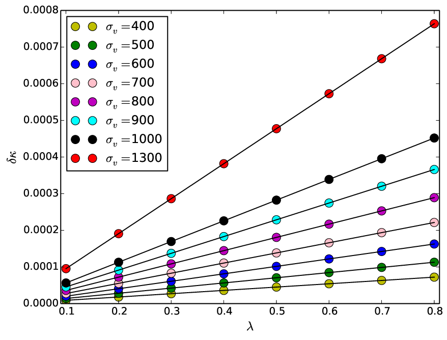
In the upper right panel of Fig. 3, the two regions can be clearly seen in two different colors. In Fig. 4, we evaluate the dependence of on the halo velocity dispersion and the rotation parameter . To do so, we generate maps induced by gravitomagnetic effects given by Eq. (14) and measure as described above. We see that gets bigger as or gets bigger. For a halo with velocity dispersion of km/s and rotation parameter of , can be comparable in size to at the edge of the halo.
We now look for a simple functional form for . As for a SIS profile, there is no rotation if there is no velocity dispersion, depends at leading order on . We measure on a grid of points of (, ) and fit with the following ansatz:
| (16) |
where we get , an overall normalization that can be considered as the typical magnitude of gravitomagnetic effects from rotating halos. Eq. (16) shows that there is a strong degeneracy between and : they are thus strongly dependent on observations.
We can also express Eq. (16) as a function of the halo mass:
| (17) |
where is the truncation radius defined in Eq. (6).
Taking into account the distribution of as given in Eq. (3), Eq. (16) becomes:
| (18) |
So far we have considered that the real (halo) rotation axis is perfectly aligned with the observed (tracer) rotation axis. If there is a misalignment between those two, will be reduced by a factor of , such that the misaligned is related to the aligned by:
| (19) |
For a given distribution , Eq. (19) becomes:
| (20) |
Combining Eq. (16), Eq. (19) and Eq. (20), we obtain a general expression for taking into account the scatters of both the angular momentum and the misalignement of the observed-to-real rotation axis:
| (21) |
To summarize, Eq. (19) describes gravitomagnetic distortion around a single cluster, while Eq. (21) provides an estimator for stacked clusters. We will discuss next this later case, asking ourselves if stacking multiple rotating lenses can achieve sufficient signal-to-noise ratio (SNR) for a measurements of gravitomagnetic effect. Meanwhile, we finish this section by discussing related issues on the measurements of gravitomagnetic distortion in the single cluster case.
We show the dependence of on the azimuthal angle, Eq. (19), in Fig. 5. The angular dependence (angle between the true rotation axis and an arbitrary axis) of is clear. However, this is difficult to estimate by stacking without any knowledge of the rotation axis. We will show later in Sec. IV that, we can infer the rotation axis by observing the same pattern of angular dependence as in Fig. 5. Such specific dependence can be used to distinguish gravitomagnetic distortions from other sub-leading lensing contributions, such as from halo asymmetry, biased tracers, and so on.


In particular, one should keep in mind that irregularities in the halo shapes can lead to a very different signal than the one we derived here, assuming perfect spherical symmetry and a SIS density profile. In Fig. 6, we show for illustration the measured map and values of as a function of on a typical halo identified in illustrisTNG300-300 (Nelson et al. 2018). Note that we did not add shape noise here, since for a single cluster, the shape noise will be overwhelmingly dominant. The signal is comparable in size to a gravitomagnetic distortion with =1000 km/s and =0.2, but we can see that the halo morphology leads to a very different profile for . Furthermore, the effect of biased tracers has not been taken into account here (this will be investigate in an upcoming work). However, at this stage, we expect that biased tracers will present a similar signal as the one for halos for gravitomagnetic effect, at least for isolated clusters. Thus, to hope detecting Einstein-Thirring-Lense effect in weak lensing surveys, one should consider relatively isolated clusters, i.e. with cylindrical selection (e.g. Mandelbaum et al. 2006), or isolated galaxies (e.g. Luo et al. 2020).


In the following section, we perform a suite of simulations to test the model above, with realistic shape noise of galaxies and galaxy number density to evaluate the detectability in LSST-like surveys.
III. Simulation
We simulate maps as described by Eq. (14) assuming a shape noise of 0.3 and galaxy number density of 50 per sq. arcmin following the characteristics of LSST (LSST Science Collaboration et al. 2009). In real observations, maps are reconstructed from the shear distortion field . All the simulated rotating halos are assuming SIS profiles in order to be consistent with our formulations. Thus, the error propagation of the shape noise to can be estimated in Fourier space as (Starck et al. 2011):
| (22) |
where and are defined as:
| (23) |
when and when . Propagating the shape noise of both components of , , the measured is then given by:
| (24) |
such that the error on is:
| (25) |
Here, we simply have , where is the shape noise, given that and . In this work we neglect the error and bias associated to the reconstruction algorithm. The final error that we use for our simulations is then .
We simulate five sets of stacked rotating clusters with fixed velocity dispersion of km/s. Table 1 shows the specification chosen for each simulation. The first three (Simulations 1, 2, and 3) are with rotation parameters , These values are motivated by the following. We choose from Miller et al. 2005 the C4 identification algorithm as informative reference for cluster characteristics: a cluster with richness of 36 has been identified with a velocity dispersion km/s. However, we restrict ourselves to a more conservative upper limit for the velocity dispersion of km/s from the observation of ABELL 2255 identified by the C4 identification algorithm. This corresponds to halo mass of , where is a solar mass, according to the scaling relation of Zahid et al. 2016. According to Vitvitska et al. 2002, the rotation parameter is about on average, however, faster rotating halos can be expected from a distribution such as in Eq. (3). If we consider SDSS DR7 north cap spectroscopic survey volume (deg2 after masking) within the redshift range , there are 26 clusters with halo mass . If we consider LSST-like survey with deg2 and a redshift range from 0.01 to 1, the volume is roughly 184 times the SDSS DR7 volume group catalog. This estimation is based on a recent group finder algorithm by Yang et al. 2020, who modify the halo-based group finder designed for SDSS survey to adopt the photometric only data for DESI Legacy Survey (Dey et al. 2019). The group catalog has photometric redshift ranging from 0.0 to 1.0. In that case, roughly about 4785 clusters with can be detected. For , only clusters can be detected, with mean . The number of detectable clusters further reduces to 13 for and to 3 for .
We also simulate six unrealistic cases with and velocity dispersion of 1000 km/s and 400 stacked clusters with zero scatter between the rotation axis indicator and the real rotation axis (Simulation 4). Fig. 7 shows one of the simulations for the 4th set with assuming zero scatter of on rotation axis. The last simulation (Simulation 5) is set to estimate the signal reduction from the misalignment between the true rotation axis and the tracer axis from observations.
| Simulation | (km/s) | (deg) | Num | |
|---|---|---|---|---|
| Sim 1 | 1000 | 0.0 | 412 | |
| Sim 2 | 1000 | 0.0 | 13 | |
| Sim 3 | 1000 | 0.0 | 3 | |
| Sim 4 | 1000 | 0.3-0.8 | 0.0 | 400 |
| Sim 5 | 1000 | 0.8 | [1,5,10,20,30] | 400 |

IV. Results
IV.1. Simulation results
We now investigate the detectability of gravitomagnetic distortion in weak lensing surveys by measuring on the simulations designed in previous section. The results are shown in Fig. 8.
Let us first focus on Simulations 1, 2, and 3, designed to mock LSST-like surveys: for , we have 412 cluster halos of mass , for an average of around 0.128. Only 13 clusters are found for , and 3 for . This is summarized in Table 1. As expected, we find that is smaller for Simulation 1 than for Simulations 2 and 3, as on average the rotation of halos is smaller. Nevertheless, as the number of stacked halos in Simulation 1 is bigger, the error bars are much smaller. For the other two, which only has 13 and 3 clusters, the shape noise overwhelms the signal by a factor of . In all these ‘realistic’ cases, we find null detection of gravitomagnetic effect, given that is compatible with zero within .
We perform further checks with Simulations 4 and 5. Simulation 4 is set to understand the relation between the measured and . The values of ranges from 0.3 to 0.8, for fixed number of 400 of stacked clusters. The theoretical prediction, Eq. (16), agrees with Simulation 4 data points.
Simulation 5 is designed to study the effect of a misalignment between the true rotation axis of clusters and the ones selected using observational tracers, such as the major axis of central galaxies (Okumura et al. 2009), the distribution of satellite galaxies inside clusters (Baxter et al. 2016), or spin axis of spiral galaxies (Zhang et al. 2015). In general, the tracers are misaligned with their dark counterpart. One famous case is the bullet cluster (Clowe et al. 2006), in which the baryonic distribution significantly differs the dark matter distribution inferred from weak lensing. To probe such discrepancy, we choose randomly for each cluster in Simulation 5 the misalignment angle between the tracer axis and the true rotation axis among a normal distribution centered on 0 with scatter: = 1, 5, 10, 20 and 30 degrees. We find that a 5 degrees scatter leads to a damping of , that remains consistent with the true input value denoted by the solid black line in the lower panel of Fig. 8. For larger scatters, the signal becomes too low to be detected, where even with 10 degrees scatter the signal is already consistent with zero. This highlights the importance to select precisely the tracer axis in order to extract the gravitomagnetic distortion signal.

IV.2. Observational indications
We now proceed with a rough quantification of the rotation axis and speed from the groups of galaxies of SDSS DR7 using redshift selection following Yang et al. 2007. The same method to measure can be used to measure the mean redshift of member galaxies separated by an arbitrary axis that has an angle of with respect to the true axis in two dimensional projected plane. Here, we use to denote the angle between the true rotation axis and the arbitrary axis from observations in order to distinguish it from used for simulations. The difference of the mean redshift from the two sides divided by the 2D rotation axis is given by: , where the indicate the two sides of the axis. Following Sofue 2013 in which the rotation curve of our own galaxy is found to be well fitted by a sine function, we fit with the parametrization:
| (26) |
The first term on the right hand side of the Eq. (26) is the offset of the group along the line of sight, which should be zero since we choose the central galaxies as the reference one such that the peculiar velocity of the cluster becomes zero (Hwang & Lee 2007). However, we caution that there might be uncertainties in the choice of the Brightest Central Galaxies (BCG). For our purpose, we consider that a nonzero offset will be much smaller than the error and thus can be neglected. The amplitude represents the rotation speed along the line of sight, and is the rotation axis angle with respect to the East to North. The relation between and velocity dispersion along the line of sight are related by (Danese et al. 1980):
| (27) |
where is the redshift of the BCG. With this procedure outlined above, we are thus able to extract all information to evaluate .
As an illustration, we select the richest group in Yang et al. 2007 catalog with 623 members with velocity dispersion of about 667.8km/s estimated from the scatter of as shown in Fig. 9, and with line-of-sight rotation speed of about 195.0km/s based on Eq. (26) and Eq. (27). The right upper panel of Fig. 9 illustrates that the rotation axis alignment can be measured by fitting the rotation curve using a sine function as in Eq. (26). We emphasize that, however, one also has to account for the projection effects in order to obtain a reliable measurement of the rotation axis. This will be discussed in a followup study based on the combination of observational group catalog and simulations. This leads to , which is extremely unlikely given the probability distribution given in Eq. (3) that we used for our simulations: the fraction of clusters with halo mass larger than in SDSS DR7 is about and the probability of a halo with is about 0.0002, yielding a joint probability of such cluster to appear in this catalog of only , according to the probability distribution inferred from simulations (Vitvitska et al. 2002). Yet, we note that this is still more likely than the bullet cluster. The probability of forming a bullet cluster liked object with such high colliding speed in LCDM framework is about (Lee & Komatsu 2010). The reason of such occurence may be due to the fact that the velocity dispersion of this cluster in underestimated because SDSS spectroscopic objects need to be brighter than 17.77 mag in the r band, which means that fainter members are not included. Even if we set the velocity dispersion to be 1000km/s, is still about 0.2. It thus seems that highly rotating clusters are not as rare as predicted by Vitvitska et al. 2002.
The rotation speed is the most important quantity to estimate gravitomagnetic distortion. If we assume that the rotation speed is 195.0km/s, for a cluster halo mass of , this leads to a value of . But for such a cluster, the shape noise will be of order 0.003 which is more than 10 times larger than the signal. Manolopoulou & Plionis 2017 have already started this research on the angular dependence of the line-of-sight rotation velocity and rotation axis using Monte-Carlo mocks of rotating clusters. They found that using their algorithm up to 28% clusters can be identified as rotating.


The error bars from Fig. 9 is estimated by bootstrap resampling method: we create 600 samples out of 623 member galaxies and take the distribution of mean value of each sample to estimate the velocity and error. The lower panel of Fig. 9 shows a degrees offset between the major axis of satellite distribution (red solid line) and rotation axis (blue dashed line) which is simply . This means that the major axis from satellites can not be used as rotation axis and tends to be anti-aligned with the major axis in this cluster. Note that we mention the major axis of clusters, as it is of more interests than the minor axis in the sense that it is more likely aligned with large-scale filament structure. The alignment between the two axis is another interesting study, which we will explore in the future.
In this figure we have all the information needed to extract from observational data, i.e. the velocity dispersion, , and the rotation axis. We will further explore if this can be achieved using the group catalog from Yang et al. 2007 and the SDSS DR7 shape catalog of Luo et al. 2017 (Tang et al. in prep.).
V. Conclusion
We have analyzed the Einstein-Thirring-Lense effect in lensing convergence maps around rotating halos. Making the bridge between observations and previous theoretical works (Ciufolini & Ricci 2003; Sereno 2005; Sereno 2007), we have constructed an estimator to measure the anistropic signal from gravitomagnetic effects induced by the rotation of foregrounds in weak lensing surveys. We find that this signal is two or three orders of magnitude smaller than the distortion from the static halo potential, in accordance with Cuesta-Lazaro et al. 2018.
Assuming lenses with a spherical SIS density profile, we have run a suite of simulations calibrated for LSST-like survey, for which we estimate that only about 400 clusters with relatively high rotation parameters can be found. Applying our estimator on the simulations, even by stacking rotating clusters with and velocity dispersion within the clusters of km/s, assuming perfect knowledge of the halo rotation axis. We also simulate data to test observational effects, such as the impact on the signal amplitude of a misalignment between the observational tracer axis and the halo rotation axis, finding that the signal is strongly reduced for a misalignment scatter of more than degrees.
However, we observe that the chosen characteristics for our mocks, in particular the dependence on the rotation parameter , is strongly motivated based on inputs from N-body simulations. In real observations, fast rotating clusters may not be as hard to find as in simulations. Indeed, we have further discussed methods to identify rotating clusters in maps from spectroscopic surveys. By selecting the most massive cluster from Yang et al. 2007, we have found that this cluster has an extremely big angular momentum with , which is very unlikely given the distribution we assumed for based on simulations. This serves as a preliminary indication that the story might be different in real observations: rotating halos may be more abundant and at higher speed in our universe than what simulations show, motivating to investigate further gravitomagnetic effects in the context of weak lensing. This will be explored in an upcoming work.
We finish by highlighting a number of interesting open questions related to the current work.
- •
We found that the major axis of Satellites position distribution in clusters can not be used to probe gravitomagnetic effect, as it is completely misaligned with the cluster rotation axis. However, the alignment between the major axis and the cluster rotation axis can be an interesting topic to study, as it can hint on the direction of the real rotation axis.
- •
We have sketched a procedure how to select rotating clusters in group catalog. This can be used to measure the distribution of , to see whether it is consistent with the one predicted from first principles or with the use of simulations.
- •
Modified gravity may lead to different lensing signals, in particular through the gravitomagnetic potential. Although gravitomagnetic distortions are difficult to detect, it may be interesting to study the impact of modification to gravity on frame-dragging effects, as the resulting signal may be different in shape and size.
- •
The elongation of the dark matter halo along the major axis does not introduce any signal to due to the subtractive nature of the estimator. As long as the density profile is symmetric with respect to the rotation axis, this elongation will not cause any extra .
We leave these issues to future studies.
Acknowledgement
We are grateful to X. Kong, Z. F. Sheng, D. Nagai, J. J. Zhang, A. Sen, W. Hossain and B. Dinda for valuable discussions. We have also received valuable suggestions and discussions from Marco Bruni at University of Portsmouth, Baojiu Li and Cristian Barrera-hinojosa from Durham Unviversity and we are very grateful for that. This work is supported in part by the NSFC (Nos. 11653002, 1201101448, 11961131007, 11722327, 11421303), by the CAST(2016QNRC001), by the National Youth Talents Program of China, by the Fundamental Research Funds for Central Universities, and by the USTC Fellowship for International Cooperation. WL and SP are supported by the World Premier International Research Center Initiative (WPI Initiative), MEXT, Japan. SP is supported partially by the National Key Research and Development Program of China Grant No.2020YFC2201502, and by JSPS Grant-in-Aid for Early-Career Scientist No. 20K14461. All numerics were operated on the computer clusters LINDA & JUDY in the particle cosmology group at USTC and gfarm cluster at Kavli IPMU, the University of Tokyo.
References
- Abazajian et al. (2009) Abazajian, K. N., Adelman-McCarthy, J. K., Agüeros, M. A., et al. 2009, ApJS, 182, 543
- Adamek et al. (2016) Adamek, J., Daverio, D., Durrer, R., & Kunz, M. 2016, Nature Physics, 12, 346
- Asgari et al. (2020) Asgari, M., Lin, C.-A., Joachimi, B., et al. 2020, arXiv e-prints, arXiv:2007.15633
- Bardeen & Petterson (1975) Bardeen, J. M., & Petterson, J. A. 1975, ApJ, 195, L65
- Barrera-Hinojosa & Li (2020) Barrera-Hinojosa, C., & Li, B. 2020, Journal of Cosmology and Astroparticle Physics, 2020, 007
- Barrera-Hinojosa et al. (2021) Barrera-Hinojosa, C., Li, B., Bruni, M., & He, J.-h. 2021, MNRAS, 501, 5697
- Barrera-Hinojosa & Sapone (2020) Barrera-Hinojosa, C., & Sapone, D. 2020, Journal of Cosmology and Astroparticle Physics, 2020, 037
- Bartelmann & Schneider (2001) Bartelmann, M., & Schneider, P. 2001, Phys. Rep., 340, 291
- Baxter et al. (2016) Baxter, E. J., Rozo, E., Jain, B., Rykoff, E., & Wechsler, R. H. 2016, MNRAS, 463, 205
- Birrer et al. (2020) Birrer, S., Shajib, A. J., Galan, A., et al. 2020, arXiv e-prints, arXiv:2007.02941
- Bonvin et al. (2018) Bonvin, C., Durrer, R., Khosravi, N., Kunz, M., & Sawicki, I. 2018, Journal of Cosmology and Astroparticle Physics, 2018, 028
- Bruni et al. (2014a) Bruni, M., Hidalgo, J. C., & Wands, D. 2014a, ApJ, 794, L11
- Bruni et al. (2014b) Bruni, M., Thomas, D. B., & Wands, D. 2014b, Phys. Rev. D, 89, 044010
- Cai et al. (2016) Cai, Y.-F., Capozziello, S., De Laurentis, M., & Saridakis, E. N. 2016, Reports on Progress in Physics, 79, 106901
- Cai et al. (2020) Cai, Y.-F., Khurshudyan, M., & Saridakis, E. N. 2020, ApJ, 888, 62
- Caminha et al. (2019) Caminha, G. B., Rosati, P., Grillo, C., et al. 2019, A&A, 632, A36
- Chen et al. (2019) Chen, Z., Luo, W., Cai, Y.-F., & Saridakis, E. N. 2019, arXiv e-prints, arXiv:1907.12225
- Chluba & Mannheim (2002) Chluba, J., & Mannheim, K. 2002, A&A, 396, 419
- Ciufolini & Ricci (2003) Ciufolini, I., & Ricci, F. 2003, arXiv e-prints, gr
- Clemence (1947) Clemence, G. M. 1947, Reviews of Modern Physics, 19, 361
- Clowe et al. (2006) Clowe, D., Bradač, M., Gonzalez, A. H., et al. 2006, ApJ, 648, L109
- Cuesta-Lazaro et al. (2018) Cuesta-Lazaro, C., Quera-Bofarull, A., Reischke, R., & Schäfer, B. M. 2018, MNRAS, 477, 741
- Danese et al. (1980) Danese, L., de Zotti, G., & di Tullio, G. 1980, A&A, 82, 322
- Dey et al. (2019) Dey, A., Schlegel, D. J., Lang, D., et al. 2019, AJ, 157, 168
- Gressel et al. (2019) Gressel, H. A., Bonvin, C., Bruni, M., & Bacon, D. 2019, Journal of Cosmology and Astroparticle Physics, 2019, 045
- Hezaveh et al. (2016) Hezaveh, Y. D., Dalal, N., Marrone, D. P., et al. 2016, ApJ, 823, 37
- Hikage et al. (2019) Hikage, C., Oguri, M., Hamana, T., et al. 2019, PASJ, 71, 43
- Huchra et al. (1985) Huchra, J., Gorenstein, M., Kent, S., et al. 1985, AJ, 90, 691
- Hwang & Lee (2007) Hwang, H. S., & Lee, M. G. 2007, ApJ, 662, 236
- Keeton (2001) Keeton, C. R. 2001, arXiv e-prints, astro
- Laureijs et al. (2011) Laureijs, R., Amiaux, J., Arduini, S., et al. 2011, arXiv e-prints, arXiv:1110.3193
- Lee & Komatsu (2010) Lee, J., & Komatsu, E. 2010, ApJ, 718, 60
- Liao (2019) Liao, K. 2019, ApJ, 871, 113
- Lou et al. (2016) Lou, Z., Liang, M., Yao, D., et al. 2016, in Society of Photo-Optical Instrumentation Engineers (SPIE) Conference Series, Vol. 10154, Society of Photo-Optical Instrumentation Engineers (SPIE) Conference Series, 101542A
- LSST Science Collaboration et al. (2009) LSST Science Collaboration, Abell, P. A., Allison, J., et al. 2009, arXiv e-prints, arXiv:0912.0201
- Lu et al. (2018) Lu, T., Luo, W., Zhang, J., et al. 2018, AJ, 156, 14
- Luo (2021) Luo, W. 2021, Gravitomagnetic effect on weak lensing kappa map, doi:10.5281/zenodo.4445484
- Luo et al. (2017) Luo, W., Yang, X., Zhang, J., et al. 2017, ApJ, 836, 38
- Luo et al. (2018) Luo, W., Yang, X., Lu, T., et al. 2018, ApJ, 862, 4
- Luo et al. (2020) Luo, W., Zhang, J., Halenka, V., et al. 2020, arXiv e-prints, arXiv:2003.09818
- Mandelbaum et al. (2006) Mandelbaum, R., Seljak, U., Kauffmann, G., Hirata, C. M., & Brinkmann, J. 2006, MNRAS, 368, 715
- Mandelbaum et al. (2005) Mandelbaum, R., Hirata, C. M., Seljak, U., et al. 2005, MNRAS, 361, 1287
- Mandelbaum et al. (2018) Mandelbaum, R., Lanusse, F., Leauthaud, A., et al. 2018, MNRAS, 481, 3170
- Manolopoulou & Plionis (2017) Manolopoulou, M., & Plionis, M. 2017, MNRAS, 465, 2616
- Milillo et al. (2015) Milillo, I., Bertacca, D., Bruni, M., & Maselli, A. 2015, Phys. Rev. D, 92, 023519
- Miller et al. (2005) Miller, C. J., Nichol, R. C., Reichart, D., et al. 2005, AJ, 130, 968
- Mroczkowski et al. (2019) Mroczkowski, T., Nagai, D., Basu, K., et al. 2019, Space Sci. Rev., 215, 17
- Navarro et al. (1997) Navarro, J. F., Frenk, C. S., & White, S. D. M. 1997, ApJ, 490, 493
- Nelson et al. (2018) Nelson, D., Pillepich, A., Springel, V., et al. 2018, MNRAS, 475, 624
- Oguri et al. (2018) Oguri, M., Lin, Y.-T., Lin, S.-C., et al. 2018, PASJ, 70, S20
- Okumura et al. (2009) Okumura, T., Jing, Y. P., & Li, C. 2009, ApJ, 694, 214
- Padmanabhan (2002) Padmanabhan, T. 2002
- Planck Collaboration et al. (2018) Planck Collaboration, Aghanim, N., Akrami, Y., et al. 2018, arXiv e-prints, arXiv:1807.06209
- Rowe et al. (2015) Rowe, B. T. P., Jarvis, M., Mandelbaum, R., et al. 2015, Astronomy and Computing, 10, 121
- Sereno (2003) Sereno, M. 2003, Phys. Rev. D, 67, 064007
- Sereno (2005) —. 2005, MNRAS, 357, 1205
- Sereno (2007) —. 2007, MNRAS, 380, 1023
- Shajib et al. (2018) Shajib, A. J., Treu, T., & Agnello, A. 2018, MNRAS, 473, 210
- Sharon et al. (2020) Sharon, K., Bayliss, M. B., Dahle, H., et al. 2020, VizieR Online Data Catalog, J/ApJS/247/12
- Sheldon et al. (2004) Sheldon, E. S., Johnston, D. E., Frieman, J. A., et al. 2004, AJ, 127, 2544
- Sofue (2013) Sofue, Y. 2013, PASJ, 65, 118
- Starck et al. (2011) Starck, J.-L., Pires, S., & Refregier, A. 2011, MRLENS: Multi-Resolution methods for gravitational LENSing, ascl:1102.005
- Suyu et al. (2017) Suyu, S. H., Bonvin, V., Courbin, F., et al. 2017, MNRAS, 468, 2590
- Tamura et al. (2015) Tamura, Y., Oguri, M., Iono, D., et al. 2015, PASJ, 67, 72
- Thomas et al. (2015a) Thomas, D. B., Bruni, M., Koyama, K., Li, B., & Zhao, G.-B. 2015a, Journal of Cosmology and Astroparticle Physics, 2015, 051
- Thomas et al. (2015b) Thomas, D. B., Bruni, M., & Wands, D. 2015b, Journal of Cosmology and Astroparticle Physics, 2015, 021
- Thomas et al. (2015) Thomas, D. B., Bruni, M., & Wands, D. 2015, MNRAS, 452, 1727
- Troxel et al. (2018) Troxel, M. A., MacCrann, N., Zuntz, J., et al. 2018, Phys. Rev. D, 98, 043528
- Verlinde (2017) Verlinde, E. 2017, SciPost Physics, 2, 016
- Vitvitska et al. (2002) Vitvitska, M., Klypin, A. A., Kravtsov, A. V., et al. 2002, ApJ, 581, 799
- Walsh et al. (1979) Walsh, D., Carswell, R. F., & Weymann, R. J. 1979, Nature, 279, 381
- Wong et al. (2019) Wong, K. C., et al. 2019, arXiv:1907.04869
- Yang et al. (2007) Yang, X., Mo, H. J., van den Bosch, F. C., et al. 2007, ApJ, 671, 153
- Yang et al. (2020) Yang, X., Xu, H., He, M., et al. 2020, arXiv e-prints, arXiv:2012.14998
- York et al. (2000) York, D. G., Adelman, J., Anderson, John E., J., et al. 2000, AJ, 120, 1579
- Zahid et al. (2016) Zahid, H. J., Geller, M. J., Fabricant, D. G., & Hwang, H. S. 2016, ApJ, 832, 203
- Zhang et al. (2015) Zhang, Y., Yang, X., Wang, H., et al. 2015, ApJ, 798, 17