A fast and accurate physics-informed neural network reduced order model with shallow masked autoencoder
Abstract
Traditional linear subspace reduced order models (LS-ROMs) are able to accelerate physical simulations in which the intrinsic solution space falls into a subspace with a small dimension, i.e., the solution space has a small Kolmogorov -width. However, for physical phenomena not of this type, e.g., any advection-dominated flow phenomena such as in traffic flow, atmospheric flows, and air flow over vehicles, a low-dimensional linear subspace poorly approximates the solution. To address cases such as these, we have developed a fast and accurate physics-informed neural network ROM, namely nonlinear manifold ROM (NM-ROM), which can better approximate high-fidelity model solutions with a smaller latent space dimension than the LS-ROMs. Our method takes advantage of the existing numerical methods that are used to solve the corresponding full order models. The efficiency is achieved by developing a hyper-reduction technique in the context of the NM-ROM. Numerical results show that neural networks can learn a more efficient latent space representation on advection-dominated data from 1D and 2D Burgers’ equations. A speedup of up to for 1D Burgers’ and a speedup of for 2D Burgers’ equations are achieved with an appropriate treatment of the nonlinear terms through a hyper-reduction technique. Finally, a posteriori error bounds for the NM-ROMs are derived that take account of the hyper-reduced operators.
keywords
nonlinear manifold solution representation, physics-informed neural network, reduced order model, nonlinear dynamical system, hyper-reduction1 Introduction
Physical simulations are influencing developments in science, engineering, and technology more rapidly than ever before. However, high-fidelity, forward physical simulations are computationally expensive and, thus, make intractable any decision-making applications, such as design optimization, inverse problems, optimal controls, and uncertainty quantification, for which many forward simulations are required to explore the parameter space in the outer loop.
To compensate for the computational expense issue, the projection-based reduced order models (ROMs) take advantage of both the known governing equation and the data. ROMs generate the solution data from the corresponding physical simulations and then compress the data to find an intrinsic solution subspace, which is represented by a linear combination of basis vectors, i.e., LS-ROMs. This condensed solution representation is plugged back into the (semi-)discretized governing equation to reduce the number of unknowns, resulting in an over-determined system, i.e., more equations than unknowns. Note that the full governing equations are used to constrain the LS-ROM through this substitution. Therefore, this can be considered as a physics-informed surrogate model. Additionally, the existing numerical methods for the corresponding full order model (FOM) is utilized in the LS-ROM solution process. Therefore, the LS-ROM fully respects the original discretization of the governing equations that describe/approximate the underlying physical laws, unlike black-box approaches.
The LS-ROM approach has been successfully applied to many problems and applications, including, but not limited to, rocket nozzle shape design [2], flutter avoidance wing shape optimization [16], topology optimization of wind turbine blades [20], porous media flow/reservoir simulations [29, 35, 74], computational electro-cardiology [73], inverse problems [28], shallow water equations [76, 66], computing electromyography [51], spatio-temporal dynamics of a predator–-prey systems [23], and acoustic wave-driven microfluidic biochips [3]. A survey paper for the projection-based LS-ROM techniques can be found in [5].
In spite of its successes, the linear subspace solution representation suffers from not being able to represent certain physical simulation solutions with a small basis dimension, such as advection-dominated or sharp gradient solutions. This is because LS-ROMs work only for physical problems in which the intrinsic solution space falls into a subspace with a small dimension, i.e., the solution space has a small Kolmogorov -width. Unfortunately, even though problems that are advection-dominated or have sharp gradient solutions are important, they do not have small Kolmogorov -width. Such physical simulations include, but are not limited to, the hyperbolic equations with high Reynolds number, the Boltzmann transport equations, and the traffic flow simulations.
Therefore, there have been many attempts to build efficient ROMs for the advection-dominated or sharp gradient problems. The attempts can be divided mainly into two categories: the first one is to enhance the solution representability of the linear subspace by introducing some special treatments and adaptive schemes and the second one is to replace the linear subspace solution representation with the nonlinear manifold.
The effort of enhancing the solution representability of the linear subspace includes the artificial viscosity, the Petrov–Galerkin projection applied to the computational fluid dynamics problems [13, 12, 19], the residual discrete empirical interpolation approach to handle the Navier-–Stokes equations with a large Reynolds number [72], and the space–time ROM [17, 18, 67] where the temporal as well as spatial dimensions were reduced to maximize the compressibility even with the advection-dominated problems. A dictionary-based model reduction method was developed in [1] where minimization is used to project onto the reduced linear subspace. A fail-safe -adaptive algorithm was developed in [9] where the reduced linear subspace basis vectors are broken algebraically to enrich the solution subspace. The shifted proper orthogonal decomposition (POD) was introduced to address the issue that arises from the advection-dominated problems [60] where a transport operator is incorporated within the POD process. The drawback with this approach is that the speed of the transport operator must be known a priori. In a similar spirit, the transport reversal was introduced in [61], which was inspired by the template fitting [38]. The windowed least-squares Petrov–Galerkin model reduction for dynamical systems with implicit time integrators is introduced in [53], which can overcome the challenges arising from the advection-dominated problems by representing only a small time window with a local ROM. In order to capture the sharp gradient accurately, many approaches use localization strategies. The examples of such methods include the online adaptive bases and sampling approach in [56] and [21]. Transformed snapshot interpolation method was also developed in [70] to capture a sharp gradient in the solution, by introducing a new transform discretization near singularities.
Even though all the approaches mentioned above do show some remedies of overcoming the challenges that arise from the advection-dominated problems, the solution representability of the linear subspace is still limited in a sense that the treatments introduced in the methods above are problem-specific and require some a priori knowledge, such as advection direction. In order to maximize the representability and make the methodology as general as possible, it seems unavoidable to transition from the linear subspace to a nonlinear manifold solution representation.
There are many works available in the current literautre that looked into the nonlinear manifold solution represenation in physical simulations. Many of them treat the weights and biases of a neural network (NN) to be unknowns in the solution process. For example, Lagaris, et al., used a single output NN as an argument for trial functions and minimized the partial/ordinary differential equation (PDE/ODE) residual norm [41], where the weights of the NNs are used as optimization variables. Dissanayake and Phan-Thien used the universal approximator of NNs as a solution representation for solving PDEs. They also used the weights of the NNs as parameters as in the work by Lagaris, et al. [24]. A similar method was also applied to a plasma equilibrium solver [68]. Meade and Fernandez used hard limit transfer functions for linear ordinary differential equations [50]. However, these approaches can introduce too many unknowns because all the wieghts and biases need to be found during the PDE/ODE solution process.
Recently, similar attempts have been made to incorporate physical laws into NN-based surrogate models —- so called physics-informed surrogate models, where the weights and biases of the NN are determined in the training phase. Such models include, but are not limited to, attempts to mimic temporal evolution by incorporating a time integrator in a loss function [59, 15, 36, 47, 4] and to represent the solution with a trained NN [59, 77, 6], the deep Galerkin method [65], approximating spatial gradient functions with a multilayer feedforward NN [30], DeepONet [48], DeepXDE [49], fractional physics-informed NNs (fPINNs) [52], PINNs with uncertainty quantification [75], and Deep Ritz method of minimizing the energy functional with trial functions of NNs [69, 31]. However, inclusions of NNs in the governing equations of the underlying physical laws, such as those above, do not take advantage of the existing numerical methods for high-fidelity physical simulations.
Recently, a neural network-based ROM is developed in [43], where the weights and biases are determined in the training phase and the existing numerical methods are utilized in their models. The same technique is extended to preserve the conserved quantities in the physical conservation laws [42]. However, their approaches do not achieve any speed-up with respect to the corresponding FOM because the nonlinear terms that still scale with the FOM size need to be updated every time step or Newton step.
Two interesting papers were written by Rim, et al., recently. First of all, manifold approximations via transported subspaces in [62] introduced a nonlinear solution representation by explicitly composing global transport dynamics with locally linear approximations of the solution manifolds. However, their approach is only applicable to 1D problem for now. The other work by Rim, et al., is the depth separation for reduced deep networks in nonlinear model reduction [63], where they applied a compression technique on weight matrices and bias vectors to achieve the reduced deep networks.
We present a fast and accurate physics-informed neural network ROM with a nonlinear manifold solution representation, i.e., the nonlinear manifold ROM (NM-ROM). We train a shallow masked autoencoder with solution data from the corresponding FOM simulations and use the decoder as the nonlinear manifold solution representation. Our NM-ROM is different from the aformentioned physics-informed neural networks in that we take advantage of the existing numerical methods of solving PDE/ODEs in our approach. Furthermore, our NM-ROM is different from the neural network-based ROM of [43] in a sense that we use a shallow masked autoencoder, while they used a deep convolutional autoencoder. The choice of the shallow masked NN over the deep convolutional NN is determined by the efficiency of the hyper-reduction technique we have developed.
1.1 Nomenclature
We use the following nomenclature/abbreviation for various ROMs throughout the paper:
- •
FOM: full order model
- •
LS-ROM: linear subspace reduced order model
- •
LS-Galerkin: linear subspace Galerkin
- •
LS-LSPG: linear subpsace least-squares Petrov–Galerkin
- •
LS-Galerkin-HR: linear subspace Galerkin hyper-reduction
- •
LS-LSPG-HR: linear subspace least-squares Petrov–Galerkin hyper-reduction
- •
NM-ROM: nonlinear manifold reduced order model
- •
NM-Galerkin: nonlinear manifold Galerkin
- •
NM-LSPG: nonlinear manifold least-squares Petrov–Galerkin
- •
NM-Galerkin-HR: nonlinear manifold Galerkin hyper-reduction
- •
NM-LSPG-HR: nonlinear manifold least-squares Petrov–Galerkin hyper-reduction
These ROMs form a hierarchy that is depicted in Fig. 1.

1.2 Organization of the paper
We organize the subsequent sections by starting to discuss some background materials in Section 2, where the FOM is stated in Section 2.1 and two LS-ROMs, i.e., LS-Galerkin and LS-LSPG, are described in Sections 2.2.2 and 2.2.3, respectively. Our NM-ROM is introduced in Section 3, where the nonlinear manifold solution representation is explained in Section 3.1. The shallow masked autoencoder that is used for the solution representation is described in Section 3.2. The NM-Galerkin is explained in Section 3.3 and the NM-LSPG is descirbed in Section 3.4. The hyper-reduction technique that enables the NM-ROM to achieve a speed-up is elaborated in Section 4. The error analysis is presented in Section 5. Finally, the performance of our NM-ROM is demonstrated in two numerical experiments in Section 6. Finally, the paper is concluded with summary and discussion in Section 7.
2 Background
2.1 Full order model
A parameterized nonlinear dynamical system is considered, characterized by a system of nonlinear ordinary differential equations (ODEs), which can be considered as a resultant system from semi-discretization of Partial Differential Equations (PDEs) in space domains
| (2.1) |
where denotes time with the final time , and denotes the time-dependent, parameterized state implicitly defined as the solution to problem (2.1) with . Further, with denotes the velocity of , which we assume to be nonlinear in at least its first argument. The initial state is denoted by , and denotes parameters in the domain .
A uniform time discretization is assumed throughout the paper, characterized by time step and time instances for with , , and . To avoid notational clutter, we introduce the following time discretization-related notations: , , , and , where , and are defined in Section 2.2.
Implicit time integrators are considered as time discretization methods. To illustrate this, we mainly consider the backward Euler time integrator for an implicit scheme. Several other time integrators are shown in Appendix A.
The implicit Backward Euler (BE) method numerically solves Eq. (2.1), by solving the following nonlinear system of equations for at -th time step:
| (2.2) |
Eq. (2.2) implies the following subspace inclusion:
| (2.3) |
By induction, we conclude the following subspace inclusion relation:
| (2.4) |
which shows that the span of nonlinear term snapshots is included in the span of solution snapshots. The residual function with the backward Euler time integrator is defined as
| (2.5) | ||||
2.2 Linear subspace reduced order model (LS-ROM)
Many projection-based reduced order models with linear subspace solution representation can be considered for nonlinear dynamical systems. We consider Galerkin and least-squares Petrov-Galerkin projection methods, which are the most relevant to our proposed method, i.e., NM-ROM.
2.2.1 Linear subspace solution representation
The linear subspace reduced order model approach applies spatial projection using a subspace with . Using this subspace, it approximates the solution as (i.e., in a trial subspace) or equivalently
| (2.6) |
and the time derivative of the solution as
| (2.7) |
where denotes a reference solution and denotes a basis matrix and denotes the generalized coordinates. The initial condition for the generalized coordinate, , is given by .
For constructing , Proper Orthogonal Decomposition (POD) is commonly used. POD [7] obtains from a truncated Singular Value Decomposition (SVD) approximation to a FOM solution snapshot matrix. It is related to principal component analysis in statistical analysis [34] and Karhunen–Loève expansion [46] in stochastic analysis. POD forms a solution snapshot matrix, , where is a solution state at -th time step with parameter for and . Then, POD computes its thin SVD:
| (2.8) |
where and are orthogonal matrices and is a diagonal matrix with singular values on its diagonals. Then POD chooses the leading columns of to set (i.e., , where is -th column vector of ). The POD basis minimizes over all with orthonormal columns, where denotes the Frobenius norm of a matrix , defined as with being an -th element of . Since the objective function does not change if is post-multiplied by an arbitrary orthogonal matrix, the POD procedure seeks the optimal –-dimensional subspace that captures the snapshots in the least-squares sense. For more details on POD, we refer to [33, 40].
2.2.2 Linear subspace Galerkin projection
We derive LS-Galerkin using time continuous residual minimization. First, we rewrite FOM ODE Eq. (2.1) as
| (2.9) |
where with denotes the time continuous residual. Here, we denote as time derivative of for notational simplicity. Replacing with given by Eq. (2.6) and with given by Eq. (2.7) leads to the following residual function with the reduced number of unknowns
| (2.10) |
where with denotes the time continuous residual. Note that is an over-determined system. Therefore, it is likely that no solution exists. To close the system, we minimize the squared norm of the residual vector function:
| (2.11) |
with . The solution to Eq. (2.11) leads to the LS-Galerkin
| (2.12) |
Applying a time integrator to Eq. (2.12) leads to a fully discretized reduced system, denoted as the reduced OE. Note that the reduced OE has unknowns and equations. If an implicit time integrator is applied, a Newton–type method can be applied to solve for unknown generalized coordinates each time step. If an explicit time integrator is applied, time marching updates will solve the system. However, we cannot expect any speed-up because the size of the nonlinear term and its Jacobian, which need to be updated for every Newton step, scales with the FOM size. In order to handle this issue, the hyper-reduction will be applied (see Section 4.2.1)
2.2.3 Linear subspace least-squares Petrov–Galerkin projection
The Least-Squares Petrov–Galerkin (LSPG) method projects a fully discretized solution space onto a trial subspace. That is, it discretizes Eq. (2.1) in time domain and replaces with for in residual functions defined in Section 2.1 and Appendix A. Here, we consider only implicit time integrators because the LSPG projection is equivalent to the Galerkin projection when an explicit time integrator is used as shown in Section 5.1 in [10]. The residual functions for implicit time integrators are defined in (2.5), (A.6), and (A.8) for various time integrators. For example, the residual function with the backward Euler time integrator11 1 Although the backward Euler time integrator is used extensively in the paper for illustrative purposes, many other time integrators introduced in Appendix A can be applied to all the ROM methods dealt in the paper in a straight forward way. after the trial subspace projection becomes
| (2.13) | ||||
The basis matrix can be found by the POD as in the Galerkin approach. Note that Eq. (2.13) is an over-determined system. To close the system and solve for the unknown generalized coordinates, , the LSPG takes the squared norm of the residual vector function and minimize it at every time step:
| (2.14) | ||||
The Gauss–Newton method with the starting point is applied to solve the minimization problem (2.14) in LSPG. However, as in the Galerkin approach, a hyper-reduction, which will be discussed in Section 4.2.2, is required for a speed-up due to the presence of the nonlinear residual vector function that scales with the full order model size.
3 Nonlinear manifold reduced order model (NM-ROM)
A projection-based reduced order model with nonlinear manifold solution representation is introduced in this section. The ROM formulation with nonlinear manifold solution representation is introduced in Section 3.1. Section 3.2 describes how we construct the neural network that is used as a nonlinear manifold solution representation. As in the LS-ROMs of Section 2.2, Galerkin and least-squares Petrov–Galerkin projections will be applied in Sections 3.3 and 3.4. Finally, the hyper-reduction for the NM-ROM is described in Section 4.
3.1 Nonlinear manifold solution representation
The NM-ROM applies solution representation using a nonlinear manifold , where with denotes a nonlinear function that maps a latent space of dimension to the full order model space of dimension, . That is, the NM-ROM approximates the solution in a trial manifold as
| (3.1) |
and the time derivative of the solution as
| (3.2) |
where denotes the generalized coordinates. The initial condition for the generalized coordinate, , is given by , where (i.e., ). The details about the nonlinear functions, and , are presented in Section 3.2.
3.2 Shallow masked autoencoder
In this section, we present the approach for constructing a nonlinear manifold. Here, we use an autoencoder, , in the form of a feedforward neural network, that is trained to reconstruct its input. The autoencoder architecture is composed of an encoder, and a decoder, . The encoder maps a high dimensional input, to a low-dimensional latent vector, , i.e., , and the decoder then maps the latent vector to , i.e., , where . Therefore, we have
| (3.3) |

The main idea behind an autoencoder is that it forces the model to learn salient features by compressing the input into a low-dimensional space and then reconstructing the input.
The universal approximation theorem [22, 57], proves that functions of the form,
| (3.4) |
where are weights, is a bias, is a non-polynomial activation function, is an input and is an output, can approximate any continuous, real-valued function arbitrarily well. Eq. (3.4) is a simple, single hidden layer neural network with a non-polynomial activation function. Its input dimension is , width of the hidden layer is , and output dimension is . We construct two single hidden layer neural networks, one is the encoder, , and the other is the decoder, . For non-polynomial activation functions, a sigmoidal function given by
| (3.5) |
or a swish function given by
| (3.6) |
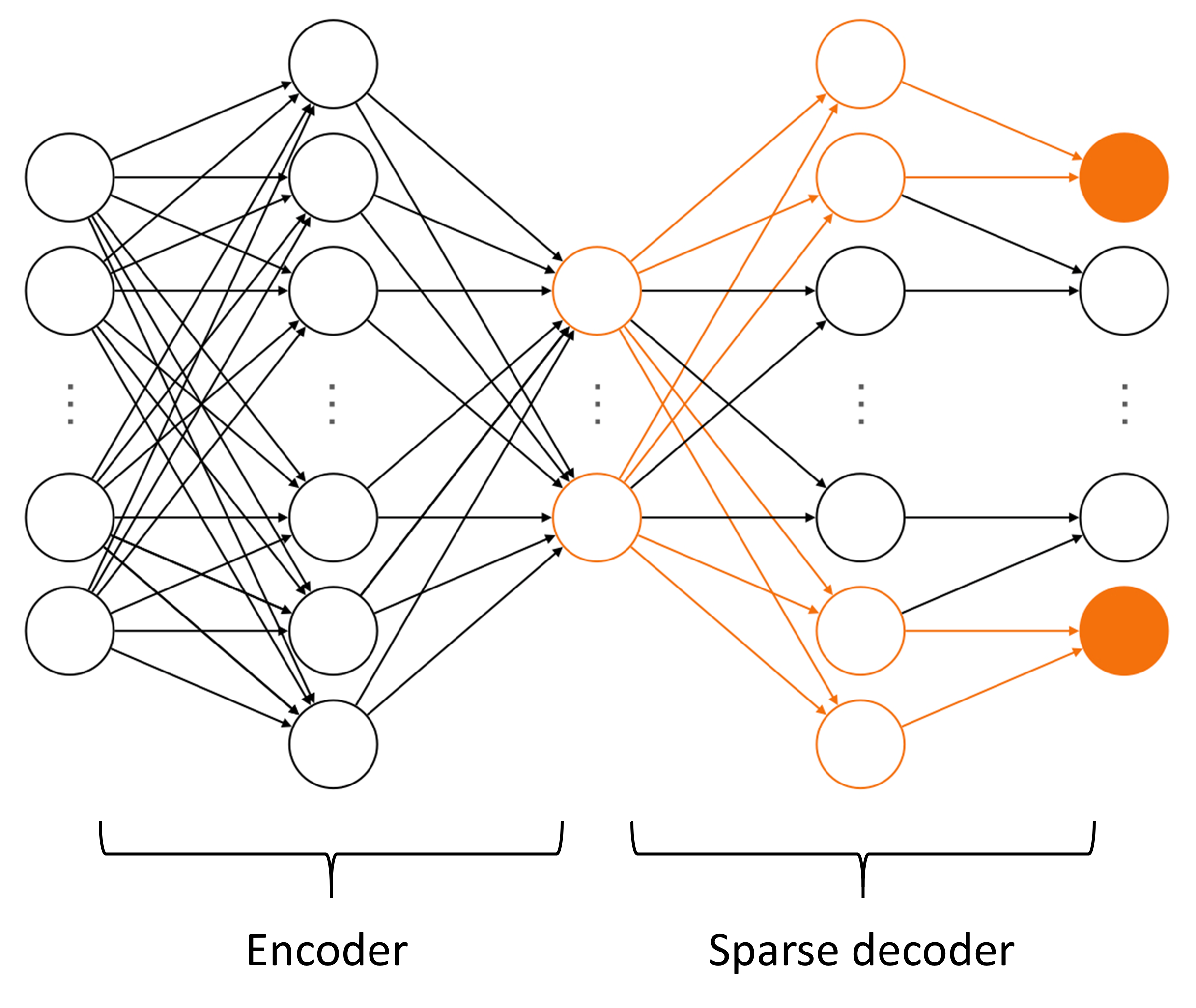
are used. We use a non-deep neural network for the decoder because the decoder and its Jacobian are computed many times during the ROM computation. In order for this computation to be on par with POD methods, it is necessary to limit the depth of the decoder network. The dimension of the encoder input and the decoder output is and the dimension of the encoder output and the decoder input is . The width of the encoder and decoder are hyper-parameters. The first layers of the encoder and decoder are fully-connected layers, where the nonlinear activation functions are applied and the last layer of the encoder is fully-connected layer with no activation functions. The last layer of the decoder is either fully-connected layer or sparsely-connected layer with no activation functions. These network architectures are shown in Fig. 3.

Then, combining the encoder and the decoder yields the autoencoder which can be trained to learn the identity mapping in an unsupervised manner because the desired output is the input. During the training phase, the error measured by
| (3.7) |
where is solution snapshot matrix and is a reconstructed solution snapshot matrix, is minimized by optimizing learnable parameters (i.e., weights and bias) in the two networks. The error is back-propagated through the networks and the gradient with respect to the learnable parameters are computed by using the chain rule [64, 54, 71]. Then, the parameters are updated in the steepest descent direction with respect to the gradient. Here, ADAM [37], a variant of stochastic gradient descent (SGD), is used to approximate the gradient with a few data samples to make training process faster. Stochastic gradient noise helps the neural network avoiding over-fitting [8]. Furthermore, graphics processing units (GPUs) are utilized to parallelize the autonencoder’s training by simultaneously approximating multiple snapshots [58]. In practice, a dataset is usually normalized before the training process. Here, we normalize the dataset (i.e., solution snapshots) in the following way:
| (3.8) |
where is a column vector of the dataset matrix and denotes the element-wise product. and are directly computed from the dataset along each feature direction such that ranges either or .
After data normalization, an autoencoder can be trained to learn the identity mapping with the normalized dataset. Now, a normalized encoder maps from a high dimensional normalized input to a low dimensional latent vector in the form:
| (3.9) |
and a normalized decoder maps from the low dimensional latent vector to a reconstructed normalized input in the form:
| (3.10) |
Next, the encoder and the decoder can be written by
| (3.11) | ||||
| (3.12) |
where and denote the element-wise product and division, respectively. Moreover, the row-wise product of and the first layer weight matrix of yields the scaled encoder . Likewise, the row-wise division of and the last layer weight matrix of gives us the scaled decoder . Finally, the encoder and the decoder are given by
| (3.13) | ||||
| (3.14) |
We set the decoder as the nonlinear manifold solution representation discussed in Section 3.
The scaled decoder can be written in the form
| (3.15) |
where and are weight matrices, is a bias vector, and is an element-wise activation function. The decoder can have more than two hidden layers (i.e., deep network). However, we use the single layer decoder (i.e., shallow network) because the Jacobian computation of the multiple hidden layer decoder involves multiple matrix–-matrix multiplications. The output layer of the decoder is fully-connected as depicted in Fig. 3 (a) (i.e., is a dense matrix), which means all nodes in the previous layer are required to compute even one element of the output vector. We apply a sparsity mask on the output layer of the decoder. Then, sampling a subset of the output vector doesn’t need all nodes in the previous layer as depicted in Fig. 3 (b). Thus, more speed-up can be achieved by a hyper-reduction technique that is described in Section 4. For example, the orange color nodes in Fig. 3 show the required nodes when the first and the last elements of the output are selected, which are represented as solid orange disks. To create a sparsely connected layer, we use a mask matrix which contains either zero or one as shown in Fig. 4. By element-wise product , a sparse weight matrix is obtained. The mask matrix is constructed to reflect local connectivity as in the Laplacian operator approximated by the central difference scheme in Finite Difference Method. The autoencoder composed of the encoder and the sparse decoder is trained by using custom pruning in PyTorch [55] pruning module.

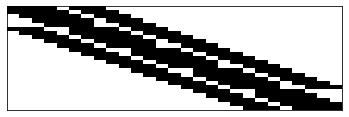
In the autoencoder, the number of learnable parameters (i.e., weights and bias) is determined by the number of nodes in the hidden layers in the encoder and the decoder, dimension of latent vector, and the sparsity in the mask matrix. The sparsity is determined by how many nodes in the hidden layer are used to compute one element of the output and how many nodes in the hidden layer are shared for neighboring elements of the output. To generate a mask matrix for 1D problem, we use two variables and , where denotes the number of nodes in the hidden layer to compute one output element (width of the block in each row in Fig. 4(a)) and denotes the amount by which the block shifts. For example, at the th row, th column is one and the others are zero. For a mask of the 2D problem, we create a building matrix in the same way as the mask matrix for 1D problem. Then, we add all rows neighboring th row (e.g., 5-point stencil for 2D and 7-point stencil for 3D) to th row and change nonzero values to one. Note that the mask matrix for 2D problem as in Fig. 4(b) looks similar to 2D finite difference Laplacian operator.
There is no way to determine these hyper-parameters a priori. If the number of learnable parameters is not enough, the decoder is not able to represent the nonlinear manifold well. On the other hand, too many learnable parameters may result in over-fitting, so the decoder is not able to generalize well, which means the trained decoder can’t be used for problems whose data is unseen, i.e., the predictive case. To avoid over-fitting, there are two options to consider. In the first option, one first divides the data into two sets, i.e., train and test sets. Then, the autoencoder is trained using the train set only and is tested for the generalization ability using the test set. If the mean squared error on the test and train sets are very different, the over-fitting occurs and we should reduce the number of learnable parameters [39].
The second option of avoiding the overfitting is to use Akaike’s information criteria (AIC) which is given by
| (3.16) |
where , is the total number of learnable parameters, and is the number of elements in the data set matrix (i.e., ). If one minimizes only the first term of AIC, then an over-fit network will be obtained. On the other hand, if one minimizes only the second term of AIC, i.e., , then the network will not fit the training distribution. Therefore, the minimum of AIC helps train a model that is not over-fit and generalizes well. [45, 39]. However, finding the minimum of AIC requires a lot more training processes than the first option above. Because of randomness in training, e.g., the random initialization of weights and bias in neural networks and SGD optimization method, will be different for every training process even with the same and the dataset matrix. Therefore, AIC needs to be averaged over several training for each to find the minimum of AIC.
Because of the practicality of the first option of avoiding the overfitting over the second option, we use the first option in our numerical experiments. For example, as shown in Fig. 5, the mean squares error on the test and train data sets are very close. This implies that the trained autoencoder is not over-fit.
3.3 Nonlinear manifold Galerkin projection
We derive NM-Galerkin using time continuous residual minimization. Replacing with given by Eq. (3.1) and with given by Eq. (3.2) in Eq. (2.9) leads to the following residual function with the reduced number of unknowns
| (3.17) |
Note that Eq. (3.17) is an over-determined system. Therefore, it is likely that no solution exists. To close the system, we minimize the squared norm of the residual vector function:
| (3.18) |
with . The solution to Eq. (3.18) leads to the NM-Galerkin
| (3.19) |
where the Moore–Penrose inverse of a matrix with full column rank is defined as .
Applying a time integrator to Eq. (3.19) leads to a fully discretized reduced system, denoted as the reduced OE. Note that the reduced OE has unknowns and equations. If an implicit time integrator is applied, a Newton–type method can be applied to solve for unknown generalized coordinates each time step. If an explicit time integrator is applied, time marching updates will solve the system. However, we cannot expect any speed-up because the size of the nonlinear terms and their Jacobians, which need to be updated for every Newton step, scales with the FOM size. In order to handle this issue, the hyper-reduction will be applied (see Section 4.3.1).
3.4 Nonlinear manifold least-squares Petrov–Galerkin projection
Alternatively, the nonlinear manifold least-squares Petrov–Galerkin (NM-LSPG) approach projects a fully discretized solution space onto a trial manifold. That is, it discretizes Eq. (2.1) in time domain and replaces with for in residual functions defined in Section 2.1 and Appendix A. Here, we consider only implicit time integrators for simplicity. See Ref. [44] for other types of time integrators. The residual functions for several implicit time integrators are defined in (2.5), (A.6), and (A.8). For example, the residual function with the backward Euler time integrator1 after the trial manifold projection becomes
| (3.20) | ||||
The nonlinear manifold can be found by training the autoencoder as described in Section 3.2. Note that Eq. (3.20) is an over-determined system. Therefore, it is likely that no solution exists. To close the system and solve for the unknown generalized coordinates, , the NM-LSPG takes the squared norm of the residual vector function and minimizes it at every time step:
| (3.21) | ||||
The Gauss–Newton method with the starting point is applied to solve the minimization problem (3.21). However, as in the Galerkin approach, a hyper-reduction which will be discussed in Section 4.3.2 is required for a speed-up due to the presence of the nonlinear residual vector function that scales with the full order model size. More specifically, , , and their Jacobians are needed to be updated whenever chagnes if the backward Euler time integrator is used.
4 Hyper-reduction
As mentioned in Section 2.2 and 3, we cannot expect speed-up even though the dimension of unknowns in ROMs is small, i.e., , because the nonlinear term still scales with the full order model size. To overcome this issue, there are several hyper-reduction techniques available, e.g., [14, 25, 26, 13, 19] for LS-ROMs. These hyper-reduction techniques share a common feature and it plays an important role in the development of the hyper-reduction technique in the NM-ROMs, so we will go over one of the hyper-reduction technique that is commonly used in the LS-ROMs.
4.1 Nonlinear residual approximation
We follow the DEIM-SNS and GNAT-SNS approaches introduced in [19] where the solution snapshots, whose span includes a span of nonlinear term snapshots, are taken to build a nonlinear term basis. Then, it selects a subset of each nonlinear term basis vector to either interpolate or data-fit in a least-squares sense. In this way, it reduces the computational complexity of updating nonlinear terms in an iterative solver for nonlinear problems.
In more details, the GNAT-SNS method approximates the nonlinear residual term with gappy POD [27] as
| (4.1) |
where , , denotes the residual basis matrix and denotes the generalized coordinates of the nonlinear residual term. Here, represents a residual vector function, e.g., the backward Euler residual, , defined in Eq. (2.13). The GNAT-SNS method uses the SVD of the FOM solution snapshot matrix to construct , which reduces computational cost by avoiding another POD to a nonlinear residual term snapshots. The hyper-reduction method solves the following least-squares problem to obtain the generalized coordinates :
| (4.2) | ||||
where , , is the sampling matrix and is the th column of the identity matrix . The solution to Eq. (4.2) is given as
| (4.3) |
where the Moore–Penrose inverse of a matrix with full column rank is defined as . Therefore, Eq. (4.1) becomes
| (4.4) |
where is the oblique projection matrix. The projection matrix has a pseudo-inverse instead of the inverse because it allows the oversampling, i.e., . The hyper-reduction method does not construct the sampling matrix . Instead, it maintains the sampling indices and corresponding rows of and . This enables hyper-reduced ROMs to achieve a speed-up when it is applied to nonlinear problems.
The sampling indices (i.e., ) can be determined by Algorithm 3 of [13] for computational fluid dynamics problems and Algorithm 5 of [11] for other problems. These two algorithms take greedy procedure to minimize the error in the gappy reconstruction of the POD basis vectors . These sampling algorithms for the hyper-reduction method allows oversampling (i.e., ), resulting in solving least-squares problems in the greedy procedure. These selection algorithms can be viewed as the extension of Algorithm 1 in [14] (i.e., a row pivoted LU decomposition) to the oversampling case. The nonlinear residual term projection error associated with these sampling algorithms is presented in Appendix D of [13]. That is,
| (4.5) |
where is the triangular factor from the QR factorization of (i.e., ). For more details, please refer to [19]22 2 In this paper, GNAT-SNS in [19] is re-named as LS-LSPG-HR to emphasize the difference between the LS-ROMs and NM-ROMs..
4.2 Hyper-reduction for LS-ROM
We present formulations of LS-Galerkin-HR and LS-LSPG-HR. For numerical examples, LS-LSPG-HR is only implemented.
4.2.1 LS-Galerkin-HR
We denote the hyper-reduced linear subspace Galerkin as LS-Galerkin-HR. The LS-Galerkin-HR method approximates the nonlinear residual term with the gappy POD procedure as in Section 4.1. Therefore, the LS-Galerkin-HR method replaces the residual in (2.11) with given by Eq. (4.4). Thus, it minimizes the following least-squares problem:
| (4.6) |
with . The solution to Eq. (4.6) leads to the following reduced ODE:
| (4.7) |
Applying a time integrator to Eq. (4.7) leads to a fully discretized reduced system, denoted as the reduced OE. Note that the reduced OE has unknowns and equations. If an implicit time integrator is applied, a Newton–type method can be applied to solve for unknown generalized coordinates each time step. If an explicit time integrator is applied, time marching updates can be applied.
Note that the operator can be pre-computed once for all. We avoid constructing the sampling matrix . For example, the operator can be computed simply by extracting only the selected rows of . For the term, , only the nonlinear term elements that are selected by the sampling matrix need to be computed. This implies that we have to keep track of the rows of that are needed to compute the selected nonlinear term elements, which is usually a larger set than the rows that are selected solely by the sampling matrix, i.e., , as in the 5-point stencil or 7-point stencil in the finite difference method.
4.2.2 LS-LSPG-HR
We denote the hyper-reduced linear subspace LSPG as LS-LSPG-HR. The LS-LSPG-HR method approximates the nonlinear residual term with the gappy POD procedure as in Section 4.1. Therefore, the LS-LSPG-HR method replaces the residual in (2.14) with given by Eq. (4.4). Thus, it minimizes the following least-squares problem:
| (4.8) |
with . Note that the pseudo-inverse can be pre-computed once for all. Due to the definition of in Eq. (2.13), the sampling matrix needs to be applied to the following terms: and at every time step. The first term can be precomputed by extracting the selected rows of the basis matrix. For the second term, only the nonlinear term elements that are selected by the sampling matrix need to be computed. This implies that we have to keep track of the rows of that are needed to compute the selected nonlinear term elements, which is usually a larger set than the rows that are selected solely by the sampling matrix, i.e., , as in the 5-point stencil or 7-point stencil in the finite difference method.
4.3 Hyper-reduction for NM-ROM
There are two layers of nonlinear terms in the NM-ROM: (i) the nonlinear term in the original governing equations, i.e., in Eq. (2.1), and (ii) the decoder, which is nonlinear function of the generalized coordinates, i.e., in Eq. (3.1) and appears in the definition of residuals both for Galerkin and Petrov–Galerkin cases. The first layer nonlinear term can be treated in the same way as the LS-ROMs (see Sections 4.2.1 and 4.2.2). Now, it is the second layer nonlinear term that requires a special attention. For example, the Jacobian of the decoder needs to be evaluated at every solver iteration. Because the cost of computing the Jacobian scales with the number of learnable parameters in the decoder, we cannot expect much speed-up. As we did in the hyper-reduction process of the LS-ROMs, we have to avoid computing all the entries of the decoder or its Jacobian because they scale with the full order model size. This will be achieved by constructing a subnet that computes only the relevant outputs, which is discussed in Section 4.4. First, we state the hyper-reduced NM-ROMs, i.e., the NM-Galerkin-HR in Section 4.3.1 and the NM-LSPG-HR in Section 4.3.2. At last, the flop count estimate comparison between non-hyper-reduced and hyper-reduced models are shown at the end of Section 4.4 and their derivations are shown in Appendix B.
4.3.1 NM-Galerkin-HR
Now, we apply the hyper-reduction to the NM-Galerkin method. We denote the hyper-reduced nonlinear manifold Galerkin as NM-Galerkin-HR. The NM-Galerkin-HR method approximates the nonlinear residual term with the gappy POD procedure as in Section 4.1. Therefore, the NM-Galerkin-HR method replaces the residual in (3.18) with given by Eq. (4.4). Thus, it minimizes the following least-squares problem:
| (4.9) |
with . The solution to Eq. (4.9) leads to the NM-Galerkin-HR
| (4.10) |
Applying a time integrator to Eq. (4.10) leads to a fully discretized reduced system, denoted as the reduced OE. Note that the reduced OE has unknowns and equations. If an implicit time integrator is applied, a Newton–type method can be applied to solve for unknown generalized coordinates each time step. If an explicit time integrator is applied, time marching updates will solve the system.
Note that the pseudo inverse, , can be pre-computed once for all by extracting only the selected rows of . However, the term, , cannot be precomputed because needs to be updated every time is updated. Fortunately, we need to compute only the selected rows of by the sampling matrix . Similarly, for the term, , only the nonlinear term elements that are selected by the sampling matrix need to be computed. This implies that we have to keep track of the outputs of that are needed to compute the selected nonlinear term elements, which is usually a larger set than the outputs that are selected solely by the sampling matrix, i.e., , as in the 5-point stencil or 7-point stencil in the finite difference method.
4.3.2 NM-LSPG-HR
We apply the hyper-reduction to the NM-LSPG method discussed in Section 3.4. The hyper-reduction procedure for the nonlinear residual function after the trial manifold projection is the same as the one in Section 4.1, i.e., we replace the residual defined in (3.20) with and plug it into the minimization problem in Eq. (3.21). Then, the minimization problem becomes
| (4.11) | ||||
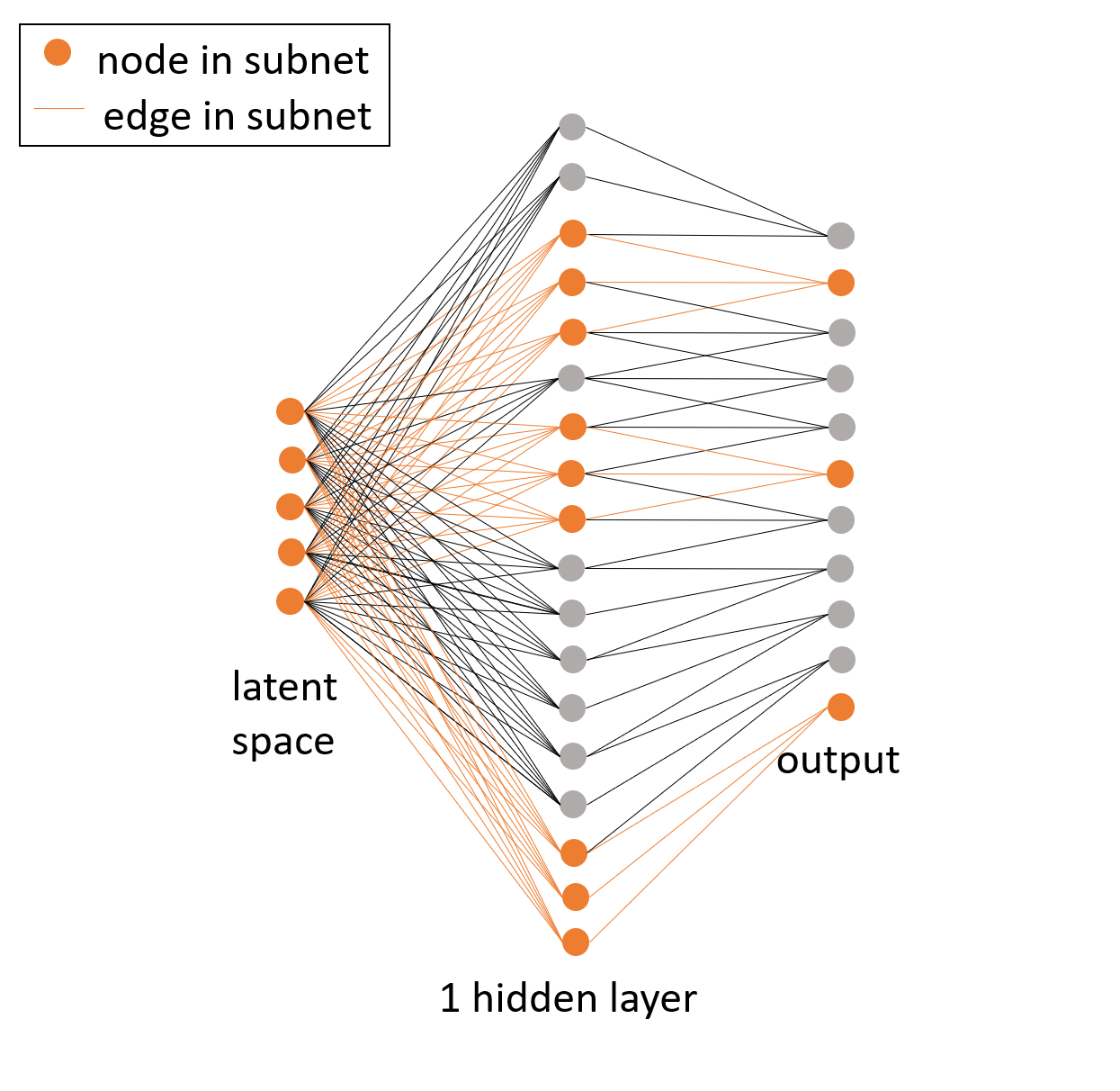
Note that the pseudo-inverse can be pre-computed once for all. Due to the definition of in Eq. (3.20), the sampling matrix needs to be applied the following two terms: and at every time step. The first term, , requires to compute only the selected outputs of the decoder. Furthermore, for the second term, only the nonlinear term elements that are selected by the sampling matrix need to be computed. This implies that we have to keep track of the outputs of that are needed to compute the selected nonlinear term elements by the sampling matrix, which is usually a larger set than the outputs that are selected solely by the sampling matrix, i.e., , as in the 5-point stencil or 7-point stencil in the finite difference method. Therefore, we build a subnet that computes only the outputs of the decoder that is required to compute the elements of the nonlinear term, . Then, with the same subnet, the outputs required for the first term, , can be extracted from the same subnet. The construction of the subnet is explained in Section 4.4.1.
4.4 Efficient Hyper-Reduction Decoder Computation
In the NM-LSPG-HR method, the residual is evaluated at the sampling points given by the hyper-reduction. We use “sample points” and “hyper-reduction indices” interchangeably throughout the paper. Evaluating the decoder and its Jacobian can be done efficiently by restricting the computation to the active paths of the outputs required to compute the selected residual elements. For example, active paths of the sparse decoder are shown in orange color in Fig. 3(b). The costs of computing the decoder and its Jacobian scale piecewise-linearly with the number of sample points because the slopes of the costs of computing the decoder and its Jacobian vs the number of sample points are different depending on how many nodes in hidden layer are shared for each sample point (see Fig. 6). The distribution of the hyper-reduction indices determines the number of overlapping nodes in hidden layer of decoder. The more the overlapping nodes in hidden layer implies the more efficient computation of the hyper-reduced decoder. If successive points are selected, overlapping of nodes in hidden layer are maximized. If the selected points are uniformly apart, then the overlapping of nodes in hidden layer is minimized. In the case of random distribution, if the number of selected points is small, the possibility of overlapping is low. Our required outputs to compute the selected residual elements after the hyper-reduction are neither successive nor uniformly separated. Thus, the cost of computing the decoder and its Jacobian would be between case 1 (successive points) and case 2 (uniformly separated points) in Fig. 6. By restricting our computation to active paths, we only compute along the subnet of the decoder network that is needed for our required outputs.
4.4.1 Construction of a subnet
To determine the sparse decoder’s active paths for given hyper-reduction indices together with additional indices required to compute the hyper-reduced residual (i.e., the neighbor indices that are used to approximate the derivatives at the sample point), denoted as , we follow the steps below:
- Step 1:
Set nonlinear activation functions to be identity functions.
- Step 2:
Replace nonzero elements of the weight matrices, and the bias vector, with one and then denote each of them as , , and , respectively. Zero elements of , , and represent non-connected edges between layers.
- Step 3:
A new decoder model, , is created in the form
(4.12) or for each layer, we can write
(4.13) (4.14) - Step 4:
Set as an input. By construction, must be all positive.
- Step 5:
Define the target vector as , where th component of the error vector, , is defined as . Then the loss function, , is defined as
(4.15) and is given by
(4.16) - Step 6:
Compute , , and using the chain rule
(4.17) (4.18) (4.19) where
(4.20) is the element-wise function. Here, we make derivatives of with respect to non-connected edges (i.e., zero elements of , , and ) zeros by element-wise multiplication with , , and because we do not consider non-connected edges as variables.
- Step 7:
Using the fact that the weights and bias that are not in the active paths do not contribute to computing , we deduce that the derivatives of with respect to such weights and bias are zero. On the other hand, the derivatives of with respect to the weights and bias that are in the support of indices in must be strictly positive because the special structure of (i.e., the same structure as the sparse decoder, , except all the nonzero weights and bias are one and the nonlinear activation functions are identity functions), choosing the all-ones vector as input vector, and defining the target vector as above should induce the positive gradient to reduce the . Thus, active path weights and bias are obtained by
(4.21) (4.22) (4.23) - Step 8:
Removing zero rows and zero columns of the active path weights and bias, , , and yields the subnet weights and bias, which are denoted as , , and , respectively. Then the subnet, is given by
(4.24)
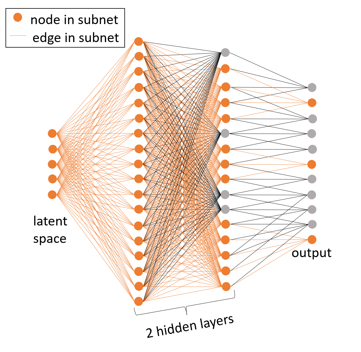
This subnet strategy works for neural networks of arbitrary depth. However, we have illustrated it in the context of the neural network with one hidden layer. It is because that is what we use to achieve enough speed up. Please see Fig. 7 for an argument of a shallow over a deep network.
Remark 4.1.
To count flops of NM-LSPG and NM-LSPG-HR, let , , , and denote FOM size, ROM size, the size of subnet output, and the number of nodes in the hidden layer to compute one output element of the sparse decoder, respectively. Then, the flop counts of NM-LSPG is and the flop counts of NM-LSPG-HR is . Thus, if is small e.g., , speed-up can be achieved. For full details, see Appendix B.
5 Error analysis
We present error analysis of the NM-LSPG-HR method. The error analysis is based on [43] and we added an oblique projection matrix for a hyper-reduction method. A posteriori discrete-time error bounds for NM-Galerkin and NM-LSPG without any hyper-reduction are derived in [43]. Here, we apply a linear multi-step method described in Appendix A.
Theorem 1.
Let with denote a sampling matrix, be an oblique projection matrix used in NM-Galerkin-HR and NM-LSPG-HR, i.e., for NM-Galerkin-HR and for NM-LSPG-HR, and denote the nonlinear residual term, which is defined by replacing with for in residual functions defined in Section 2.1 and Appendix A, e.g., the residual with the backward Euler time integrator is defined in Sections 3.4 and 4.3.2. Then, if the velocity is Lipschitz continuous with the Lipschitz constant and the time step size is sufficiently small such that , we have the following error bound
| (5.1) |
for NM-Galerkin-HR and
| (5.2) |
for NM-LSPG-HR, where coefficients define a particular linear multi-step scheme and are .
Proof.
We have
| (5.3) | ||||
| (5.4) |
where denotes FOM solution and is approximate solution.
Subtracting Eq. (5.3) from Eq. (5.4) gives
| (5.5) |
We can re-write this in the following form
| (5.6) |
Applying the reverse triangle inequality gives
| (5.7) |
Now, we use relationships
| (5.8) |
and
| (5.9) |
where and . Then, we have
| (5.10) |
If is Lipschitz continuous with and is sufficiently small such that , we have
| (5.11) |
With triangle inequality and Lipschitz continuity of , we have
| (5.12) |
Combining Eq. (5.11) and (5.12) yields
| (5.13) |
The error bound for NM-Galerkin-HR Eq. (5.1) is proved. Furthermore, noting that NM-LSPG-HR solution minimizes the term in Eq. (5.13) proves the error bound for NM-LSPG-HR Eq.(5.2). ∎
From the error bound for NM-LSPG-HR, we know that the NM-LSPG-HR solutions satisfy sequential minimization of the error bound.
6 Numerical results
We demonstrate the accuracy and speed-up of the nonlinear manifold reduced order model for two advection-dominated problems: (i) a parameterized 1D inviscid Burgers equation in Section 6.1 and (ii) a parameterized 2D viscous Burgers equation with a large Reynolds number (i.e., the advection-dominated case) in Section 6.2. The ROMs are trained with solution snapshot associated with train parameters in a parameter space and are used to predict the solution of the parameter that is not included in the train parameters. We refer this to the predictive case. The accuracy of ROM solution is assessed from its maximum relative error:
| (6.1) |
where is the corresponding FOM solution. We also introduce the projection errors for the lower bounds of LS-ROMs and NM-ROMs maximum relative errors:
| (6.2) |
for linear subspace projection and
| (6.3) |
for nonlinear manifold projection, where denotes a POD basis matrix, and the scaled decoder and the scaled encoder are a nonlinear manifold and its approximate inverse function that are obtained from an autoencoder, respectively. The computational cost is measured in terms of the CPU wall time. Specifically, timing is obtained by performing calculations on an Intel(R) Xeon(R) CPU E5-2637 v3 @ 3.50 GHz and DDR4 Memory @ 1866 MT/s. The autoencoders are trained on a NVIDIA Quadro M6000 GPU with 3072 NVIDIA CUDA Cores and 12 GB GDDR5 GPU Memory using PyTorch [55] which is the open source machine learning frame work.
6.1 1D inviscid Burgers’ equation
We consider a parameterized 1D inviscid Burgers’ equation
| (6.4) | ||||
| (6.5) | ||||
| (6.6) |
where denotes a scalar-valued time dependent state variable with the periodic boundary condition
| (6.7) |
and the initial condition
| (6.8) |
where is a parameter. Discretizing the space domain into uniform mesh gives grid points where and . We denote the discrete solutions on grid points as , where . Then, the backward difference scheme yields the semi-discretized equation which is written by
| (6.9) |
where and is in the form
| (6.10) |
where
| (6.11) |
with denoting element-wise multiplication.
For a time integrator, we use the backward Euler scheme with time step size , where is final time and is the number of time steps. We set , , and .
For the training process, we collect solution snapshots associated with the parameter such that at which the FOM is solved. Then, the number of train data points is and of the train data are used for validation purpose. We employ the Adam optimizer [37] for SGD with initial learning rate which decreases by a factor of when a training loss stagnates for successive training epochs. We set the number of nodes in the hidden layer of the encoder, , and the number of nodes in the hidden layer of the decoder, . The weights and bias of the autoencoder are initialized via Kaiming initialization [32]. The size of the batch is and the maximum number of epochs is . The training process is stopped if the loss on the validation dataset stagnates for epochs.
After the training is done, the NM-ROMs and LS-ROMs solve the Eq. (6.4) with the target parameter which is not included in the train dataset for training the autoencoder and the linear subspace. Fig. 8 shows the relative error versus the reduced dimension . It also shows the projection errors for LS-ROMs and NM-ROMs, which are defined in (6.2) and (6.3). These are the lower bounds for LS-ROMs and NM-ROMs, respectively. As expected the relative errors for the NM-ROMs are lower than the ones for the LS-ROMs. We even observe that the relative errors of NM-ROMs are even lower than the lower bounds of LS-ROMs.
To see the trends regarding the number of training parameter instances, we increase the number of parameters starting from with the fixed reduced dimension to achieve less than maximum relative error for NM-ROMs. In Fig. 9, we observe that is enough.
LS-ROMs with are able to achieve speed-up, but their accuracies are not as good as NM-ROMs. For example, LS-ROMs are about to times faster than FOM on average and have a maximum relative error of %. NM-ROMs solve the problem with less than the maximum relative error of %. For LS-ROMs, a hyper-reduction improves speed-up (e.g., to times faster than FOM) but accuracy doesn’t get better. On the other hand, NM-ROMs without a hyper-reduction do not achieve any speed-up with respect to the corresponding FOM simulation. For example, the FOM simulation takes seconds, while the NM-Galerkin and NM-LSPG with takes and seconds, respectively. Therefore, the hyper-reduction is essential to achieve a speed-up with a reasonable accuracy for the NM-ROMs. Now, we compute the maximum relative error and wall-clock time for the hyper-reduced ROMs, i.e., NM-LSPG-HR and LS-LSPG-HR, by varying the number of residual basis and residual samples with the fixed number of training parameter instances and the reduced dimension and show the results in Table 1. Although the LS-LSPG-HR can achieve a better speed-up than the NM-LSPG-HR, the relative error of the LS-LSPG-HR is too large, e.g., the relative errors of around . On the other hand, the NM-LSPG-HR achieves much better accuracy, i.e., a relative error of around , than the LS-LSPG-HR with a speedup of higher than .
| NM-LSPG-HR | LS-LSPG-HR | |||||||||||
| Residual basis | 31 | 33 | 36 | 32 | 40 | 32 | 30 | 30 | 30 | 31 | 41 | 41 |
| Residual samples | 47 | 49 | 40 | 47 | 42 | 46 | 47 | 48 | 49 | 49 | 49 | 48 |
| Max. rel. error (%) | 1.03 | 1.07 | 1.18 | 1.23 | 1.23 | 1.25 | 6.07 | 6.08 | 6.08 | 6.09 | 6.11 | 6.11 |
| Wall-clock time (sec) | 0.63 | 0.51 | 0.49 | 0.50 | 0.51 | 0.50 | 0.14 | 0.13 | 0.13 | 0.23 | 0.14 | 0.13 |
| Speed-up | 2.07 | 2.53 | 2.63 | 2.62 | 2.56 | 2.62 | 9.29 | 9.80 | 9.71 | 5.65 | 9.63 | 9.82 |


Fig. 10 shows solutions in both space and time domain of FOM, NM-LSPG-HR, and LS-LSPG-HR with the reduced dimension being . For NM-LSPG-HR, residual basis and residual samples are used and for LS-LSPG-HR, residual basis and residual samples are used. In fact, the NM-LSPG-HR is able to achieve an accuracy as good as the NM-LSPG for some combinations of the small number of residual basis and residual samples.
We look into the numerical tests to see the generalization capability of the NM-LSPG and NM-LSPG-HR, i.e., the robustness of the NM-LSPG and NM-LSPG-HR outside of the trained domain. The training sample point set, , is used to train a NM-LSPG-HR. Then the trained NM-LSPG-HR model is used to predict the following parameter points, . The residual basis dimension and the number of residual samples for each test case are given in Table 2. Fig. 11 shows the maximum relative error over the test range of the parameter points. Note that the NM-LSPG and NM-LSPG-HR are the most accurate within the range of the training points, i.e., . As the parameter points go beyond the training parameter domain, the accuracy of the NM-LSPG and NM-LSPG-HR start to deteriorate gradually. This implies that the NM-LSPG and NM-LSPG-HR have a trust region. Its trust region should be determined by an application. For example, if the application is okay with the maximum relative error of %, then the trust region of this particular NM-LSPG-HR is . However, if the application requires a higher accuracy, e.g., the maximum relative error of %, then the trust region of the NM-LSPG-HR is . Note that the average speed-up of the NM-LSPG-HR for all the test cases is (see Table 2).
| Residual basis | Residual samples | Wall-clock time (sec) | Speed-up | |
|---|---|---|---|---|
| 0.60 | 46 | 48 | 0.54 | 2.41 |
| 0.62 | 37 | 39 | 0.46 | 2.83 |
| 0.64 | 37 | 39 | 0.47 | 2.77 |
| 0.66 | 44 | 46 | 0.52 | 2.50 |
| 0.68 | 42 | 44 | 0.48 | 2.71 |
| 0.70 | 42 | 44 | 0.48 | 2.71 |
| 0.72 | 42 | 44 | 0.48 | 2.71 |
| 0.74 | 42 | 44 | 0.48 | 2.71 |
| 0.76 | 43 | 45 | 0.53 | 2.45 |
| 0.78 | 36 | 45 | 0.46 | 2.83 |
| 0.80 | 38 | 47 | 0.47 | 2.77 |
| 0.82 | 38 | 47 | 0.47 | 2.77 |
| 0.84 | 38 | 47 | 0.47 | 2.77 |
| 0.86 | 38 | 47 | 0.47 | 2.77 |
| 0.88 | 37 | 46 | 0.46 | 2.83 |
| 0.90 | 33 | 33 | 0.45 | 2.89 |
| 0.92 | 33 | 33 | 0.46 | 2.83 |
| 0.94 | 33 | 33 | 0.46 | 2.83 |
| 0.96 | 33 | 33 | 0.45 | 2.89 |
| 0.98 | 31 | 47 | 0.45 | 2.89 |
| 1.00 | 31 | 47 | 0.45 | 2.89 |
| 1.02 | 33 | 49 | 0.48 | 2.71 |
| 1.04 | 31 | 48 | 0.46 | 2.83 |
| 1.06 | 30 | 48 | 0.46 | 2.83 |
| 1.08 | 33 | 39 | 0.48 | 2.71 |
| 1.10 | 33 | 40 | 0.48 | 2.71 |
| 1.12 | 33 | 42 | 0.48 | 2.71 |
| 1.14 | 44 | 49 | 0.54 | 2.41 |
| 1.16 | 31 | 48 | 0.48 | 2.71 |
| 1.18 | 31 | 48 | 0.47 | 2.77 |
| 1.20 | 44 | 48 | 0.57 | 2.28 |
6.2 2D Burgers’ equation
We now consider a parameterized 2D viscous Burgers’ equation
| (6.12) | ||||
| (6.13) | ||||
| (6.14) | ||||
| (6.15) |
with the boundary condition
| (6.16) |
and the initial condition
where is a parameter and and denote the and directional velocities, respectively, with and defined as the solutions to Eq. (6.12), and is a Reynolds number which is set . In the case of (an advection-dominated case), the FOM solution snapshot shows slowly decaying singular values compared to the case of as shown in Fig. 12 and we observe that a sharp gradient, i.e., a shock, appears in Figs. 15(a) and 15(d).
Discretizing the space domain into and uniform meshes in and directions, respectively, gives grid points . is given by where and and is given by where and . We denote the discrete solutions on grid points as and , where and . Let . Then, the backward difference scheme for the first spatial derivative terms
| (6.21) | ||||
| (6.22) |
and the central difference scheme for the second spatial derivative terms
| (6.23) | ||||
| (6.24) |
yield the semi-discretized equation which is written by
| (6.25) | ||||
| (6.26) |
where and with superscript standing for the transpose operation and and are in the form
| (6.27) | ||||
| (6.28) | ||||
| (6.29) | ||||
| (6.30) |
where
| (6.31) | ||||
| (6.32) | ||||
| (6.33) | ||||
| (6.34) | ||||
| (6.35) | ||||
| (6.36) | ||||
| (6.37) | ||||
| (6.38) | ||||
| (6.39) | ||||
| (6.40) | ||||
| (6.41) | ||||
| (6.42) |
with and denoting the element-wise multiplication and the Kronecker product, respectively.
For a time integrator, we use the backward Euler scheme with time step size , where is the number of time steps. We set , , and .
For the training process, we collect solution snapshots associated with the parameter such that at which the FOM is solved. Then, the number of train data points is and of the train data are used for validation purpose. We employ the Adam optimizer [37] with the SGD and the initial learning rate of , which decreases by a factor of when a training loss stagnates for successive training epochs. Here, we have two autoencoders. One for vector and the other for vector. The reason why we have such two autoencoders is that we can use less memory for training process compared to one autoencoder for vector and train both of them at the same time. We set the number of nodes in hidden layer in the encoder, , and the number of nodes in hidden layer in the decoder, . The weights and bias of the autoencoder are initialized via Kaiming initialization [32] as in the first numerical example. The size of the batch is and the maximum number of epochs is . The training process is stopped if the loss on the validation dataset stagnates for epochs.
After the training is done, the NM-ROMs and LS-ROMs solve the Eq. (6.12) with the target parameter ,which is not included in the train dataset for training the autoencoder and the linear subspace. Fig. 13 shows the relative error versus the reduced dimension for both NM-ROMs and LS-ROMs. It also shows the projection errors for LS-ROMs and NM-ROMs, which are defined in (6.2) and (6.3). These are the lower bounds for LS-ROMs and NM-ROMs, respectively. As expected the relative errors for the NM-ROMs are lower than the ones for the LS-ROMs. We even observe that the relative errors of NM-LSPG are even lower than the lower bounds of LS-ROMs. One notable observation is that NM-Galerkin is not able to achieve a good accuracy, while the NM-LSPG does. Another observation is that LS-ROMs struggle more for this problem than the 1D invisid Burgers’ equations, e.g., some LS-ROMs fail to converge.
To see the trends regarding the number of training parameter instances, we increase the number of parameters starting from with the fixed reduced dimension to achieve less than maximum relative error for NM-ROMs. In Fig. 14, we observe that is enough.
Both NM-Galerkin and LS-ROMs without a hyper-reduction do not achieve any speed-up with respect to the corresponding FOM simulation. For example, the FOM simulation takes seconds, while the NM-Galerkin, NM-LSPG, LS-Galerkin, and LS-LSPG with takes , , and seconds, respectively. Although NM-LSPG is able to achieve a speed-up, it is not considerable. Therefore, the hyper-reduction is essential to achieve a considerable speed-up with a reasonable accuracy.
We compute the maximum relative error by choosing the larger of the two errors between the maximum relative error of and the maximum relative error of . We vary the number of residual basis and residual samples, with the fixed number of training parameter instances and the reduced dimension , and measure the wall-clock time. The results are shown in Table 3. Although the LS-LSPG-HR can achieve better speedup than the NM-LSPG-HR, the relative error of the LS-LSPG-HR is too large to be reasonable, e.g., the relative errors of around . On the other hand, the NM-LSPG-HR achieves much better accuracy, i.e., a relative error of around , than the LS-LSPG-HR with a good speedup, i.e., a speedup of higher than .
| NM-LSPG-HR | LS-LSPG-HR | |||||||||||
| Residual basis | 55 | 56 | 51 | 53 | 54 | 44 | 59 | 53 | 53 | 53 | 53 | 53 |
| Residual samples | 58 | 59 | 54 | 56 | 57 | 47 | 59 | 58 | 59 | 56 | 55 | 53 |
| Max. rel. error (%) | 0.93 | 0.94 | 0.95 | 0.97 | 0.97 | 0.98 | 34.38 | 37.73 | 37.84 | 37.95 | 37.96 | 37.97 |
| Wall-clock time (sec) | 12.15 | 12.35 | 12.09 | 12.14 | 12.29 | 12.01 | 5.26 | 5.02 | 4.86 | 5.05 | 4.75 | 7.18 |
| Speed-up | 11.58 | 11.39 | 11.63 | 11.58 | 11.44 | 11.71 | 26.76 | 28.02 | 28.95 | 27.83 | 29.61 | 19.58 |


Fig. 15 shows solutions at the last time step of FOM, NM-LSPG-HR, and LS-LSPG-HR with the reduced dimension being . For NM-LSPG-HR, residual basis dimension and residual samples are used and for LS-LSPG-HR, residual basis dimension and residual samples are used. Both FOM and NM-LSPG-HR show good agreement in their solutions, while the LS-LSPG-HR is not able to achieve a good accuracy. In fact, the NM-LSPG-HR is able to achieve an accuracy as good as the NM-LSPG for some combinations of the small number of residual basis and residual samples as in Section 6.1.
We look into the numerical tests to see the generalization capability of the NM-LSPG and NM-LSPG-HR, i.e., the robustness of the NM-LSPG and NM-LSPG-HR outside of the trained domain. The training sample point set, , is used to train a NM-LSPG-HR. Then the trained NM-LSPG-HR model is used to predict the following parameter points, . The residual basis dimension and the number of residual samples for each test case are given in Table 4. Fig. 16 shows the maximum relative error over the test range of the parameter points. Note that the NM-LSPG and NM-LSPG-HR are the most accurate within the range of the training points, i.e., . As the parameter points go beyond the training parameter domain, the accuracy of the NM-LSPG and NM-LSPG-HR start to deteriorate gradually. This implies that the NM-LSPG and NM-LSPG-HR have a trust region. Its trust region should be determined by an application. For example, if the application is okay with the maximum relative error of %, then the trust region of this particular NM-LSPG-HR is . However, if the application requires a higher accuracy, e.g., the maximum relative error of %, then the trust region of the NM-LSPG-HR is . Note that the average speed-up of the NM-LSPG-HR for all the test cases is (see Table 4).
| Residual basis | Residual samples | Wall-clock time (sec) | Speed-up | |
|---|---|---|---|---|
| 0.85 | 47 | 59 | 13.65 | 10.31 |
| 0.86 | 50 | 50 | 13.19 | 10.66 |
| 0.87 | 45 | 45 | 12.61 | 11.16 |
| 0.88 | 49 | 50 | 12.69 | 11.08 |
| 0.89 | 52 | 52 | 13.41 | 10.49 |
| 0.90 | 53 | 57 | 13.35 | 10.54 |
| 0.91 | 59 | 59 | 13.60 | 10.34 |
| 0.92 | 55 | 58 | 13.41 | 10.49 |
| 0.93 | 51 | 54 | 13.17 | 10.68 |
| 0.94 | 54 | 57 | 13.32 | 10.56 |
| 0.95 | 55 | 58 | 13.52 | 10.40 |
| 0.96 | 55 | 58 | 13.54 | 10.39 |
| 0.97 | 54 | 57 | 13.39 | 10.51 |
| 0.98 | 52 | 55 | 13.20 | 10.66 |
| 0.99 | 52 | 55 | 13.18 | 10.67 |
| 1.00 | 55 | 58 | 13.38 | 10.51 |
| 1.01 | 46 | 49 | 12.80 | 10.99 |
| 1.02 | 50 | 53 | 13.35 | 10.54 |
| 1.03 | 50 | 53 | 13.40 | 10.50 |
| 1.04 | 52 | 53 | 13.40 | 10.50 |
| 1.05 | 46 | 58 | 13.21 | 10.65 |
| 1.06 | 54 | 57 | 13.58 | 10.36 |
| 1.07 | 45 | 57 | 13.20 | 10.66 |
| 1.08 | 45 | 57 | 13.23 | 10.63 |
| 1.09 | 43 | 55 | 13.27 | 10.60 |
| 1.10 | 44 | 48 | 13.31 | 10.57 |
| 1.11 | 40 | 43 | 12.79 | 11.00 |
| 1.12 | 48 | 59 | 13.66 | 10.30 |
| 1.13 | 42 | 51 | 13.25 | 10.62 |
| 1.14 | 46 | 49 | 13.10 | 10.74 |
| 1.15 | 40 | 50 | 13.11 | 10.73 |
.
7 Discussion & conclusion
In this work, we have successfully developed an accurate and efficient nonlinear manifold based reduced order model. We demonstrated that the linear subspace based reduced order model is not able to represent advection-dominated or sharp gradient solutions of 1D inviscid Burgers’ equation and 2D viscous Burgers’ equation with a high Reynolds number. However, our new approach, NM-LSPG-HR, solves such problems accurately and efficiently. For 1D case, the NM-LSPG-HR method achieves a good accuracy i.e., the maximum relative error of around with the speed-up of higher than . For 2D case, the NM-LSPG-HR method was able to achieve even better accuracy, i.e., the maximum relative error of less than , with even better speed-up of around than the 1D case. We also presented a posteriori error bounds for NM-Galerkin-HR and NM-LSPG-HR. The speed-up of the NM-LSPG-HR is achieved by choosing the sparse shallow decoder as the nonlinear manifold and applying the efficient hyper-reduction computation, which can be done by constructing a subnet. Furthermore, we expect more speed-up as the FOM size increases because the difference in the computational cost between the FOM and NM-LSPG-HR increases as shown in Fig. 17.
Compared with the deep neural networks for computer vision and natural language processing applications, our neural networks are shallow with a small number of parameters. However, these networks were able to capture the variation in our 1D and 2D Burgers’ simulations. A main future work for transferring this work to more complex simulations, will be to find the right balance between a shallow network that is large enough to capture the data variance and yet small enough to run faster than the FOM. Another future work will be to find an efficient way of determining the proper size of the residual basis and the number of sample points a priori. To find the optimal size of residual basis and the number of sample points for hyper-reduced ROMs, we relied on test results. This issue is not just for NM-LSPG-HR but also for LS-LSPG-HR.
Acknowledgments
This work was performed at Lawrence Livermore National Laboratory and was supported by the LDRD program (project 20-FS-007). Youngkyu was also supported for this work through generous funding from DTRA. Lawrence Livermore National Laboratory is operated by Lawrence Livermore National Security, LLC, for the U.S. Department of Energy, National Nuclear Security Administration under Contract DE-AC52-07NA27344 and LLNL-JRNL-814844.
Appendix A Time integrators
A.1 The linear multistep methods
Applying a linear -step method to numerically solve Eq. (2.1) yields an OE characterized by the following system of nonlinear algebraic residual function that needs to be solved for the numerical solution at each time instance:
| (A.1) | ||||
| (A.2) |
where coefficients , define a particular linear multistep scheme. It is necessary for consistency to have and . Here, denotes the number of steps used by the linear multistep method at time instance . The linear multistep methods include the one-step Euler methods, the implicit Adams–Moulton methods, the explicit Adams–Bashforth methods, and the Backward Differentiation Formulas (BDFs).
The second order Adams–Bashforth (AB) method numerically solves Eq. (2.1), by solving the following nonlinear system of equations for at -th time step:
| (A.3) |
The residual function of the second AB method is defined as
| (A.4) | ||||
The second order Adams–Moulton (AM) method numerically solves Eq. (2.1), by solving the following nonlinear system of equations for at -th time step:
| (A.5) |
The residual function of the second AM method is defined as
| (A.6) | ||||
The 2-step BDF numerically solves Eq. (2.1), by solving the following nonlinear system of equations for at n-th time step:
| (A.7) |
The residual function of the two-step BDF method is defined as
| (A.8) | ||||
A.2 The midpoint Runge–Kutta method
The midpoint method, a -stage Runge–Kutta method, takes the following two stages to advance at n-th time step of Eq. (2.1):
| (A.9) | ||||
Appendix B Computational costs
Let’s denote the size of FOM and ROM as and , respectively. Because of mathematical models that require local information, we need not only the indices selected from the hyper-reduction, but also their neighbors. We denote the total number of indices as and assume , and (e.g., ). For simplicity, we assume the mask matrix for the sparse decoder has the same structure as the mask matrix for 1D Burgers equation as depicted in Section 3.2. To generate the mask matrix, two variables and are used, where denotes the number of nodes in the hidden layer to compute single output element and denotes the amount by which the block of nodes shifts. Then, the number of nodes in the hidden layer can be computed as .
B.1 Computational costs of NM-LSPG
Since the decoder is a single hidden layer neural network, the cost of the decoder and its Jacobian evaluation is and , respectively. Computing residual, , includes only element-wise vector calcualtion, resulting in . Jacobian of the residual, , can be computed using row-wise multiplication of matrix and vector because of local connectivity of mathematical model (e.g., discrete 1D and 2D Burgers equation) in . For the Gauss–Newton method, we need to construct and , which requires and , respectively. It also takes to compute each update, , iteratively. Assuming the number of Gauss–Newton iterations is in the same order for the given governing equation, we can factor out the number of iterations. Thus, the total computational costs of NM-LSPG for each time step is . With the assumption of , , and , we have .
B.2 Computational costs of NM-LSPG-HR
The size of the weight matrix connecting the hidden layer and the output layer is reduced to by , where for the best case ( successive points are selected) and for the worst case ( uniformly separate points are selected). Note that when is small, it is possible to have even for the worst case. Then, replacing with and with in the decoder and its Jacobian evaluation gives us and , respectively. Costs of computing residual, and its Jacobian, for NM-LSPG-HR are and , respectively because the sampling matrix selects elements of the residual and rows of its Jacobian without constructing the sampling matrix. For the Gauss–Newton method, we need to construct and , where is the pre-computed matrix, which require and , respectively. It also takes to compute each update, , iteratively. Assuming the number of Gauss–Newton iterations is in the same order for the given governing equation, we can factor out the number of iterations. Thus, the total computational costs of NM-LSPG-HR for each time step is . With the assumption of , we have . For the best case, , the computational costs is . Assuming , we have . For the worst case, , we have .
B.3 Computational costs of LS-LSPG
The decoder and its Jacobian are replaced with and , respectively. Thus, the cost of is and the cost of its Jacobian evaluation is zero. The costs of computing residual and its Jacobian are the same as for NM-LSPG . Also, the costs of the Gauss–Newton method is the same as in Section B.1. Assuming the number of Gauss–Newton iterations is in the same order for the given governing equation, we can factor out the number of iterations. Thus, the total computational costs of LS-LSPG for each time step is .
B.4 Computational costs of LS-LSPG-HR
For LS-LSPG-HR, we construct reduced model with the size of basis matrix being by , where . Thus, the costs of is and the cost of its Jacobian evaluation is zero. The costs of computing residual and its Jacobian are the same as for NM-LSPG-HR. Also, the costs of the Gauss–Newton method is the same as in Section B.2. Assuming the number of Gauss–Newton iterations is in the same order for the given governing equation, we can factor out the number of iterations. Thus, the total computational costs of LS-LSPG-HR for each time step is .
References
- [1] Rémi Abgrall, David Amsallem, and Roxana Crisovan. Robust model reduction by -norm minimization and approximation via dictionaries: application to nonlinear hyperbolic problems. Advanced Modeling and Simulation in Engineering Sciences, 3(1):1–16, 2016.
- [2] David Amsallem, Matthew Zahr, Youngsoo Choi, and Charbel Farhat. Design optimization using hyper-reduced-order models. Structural and Multidisciplinary Optimization, 51(4):919–940, 2015.
- [3] Harbir Antil, Matthias Heinkenschloss, Ronald HW Hoppe, Christopher Linsenmann, and Achim Wixforth. Reduced order modeling based shape optimization of surface acoustic wave driven microfluidic biochips. Mathematics and Computers in Simulation, 82(10):1986–2003, 2012.
- [4] Christian Beck, E Weinan, and Arnulf Jentzen. Machine learning approximation algorithms for high-dimensional fully nonlinear partial differential equations and second-order backward stochastic differential equations. Journal of Nonlinear Science, 29(4):1563–1619, 2019.
- [5] Peter Benner, Serkan Gugercin, and Karen Willcox. A survey of projection-based model reduction methods for parametric dynamical systems. SIAM review, 57(4):483–531, 2015.
- [6] Jens Berg and Kaj Nyström. A unified deep artificial neural network approach to partial differential equations in complex geometries. Neurocomputing, 317:28–41, 2018.
- [7] Gal Berkooz, Philip Holmes, and John L Lumley. The proper orthogonal decomposition in the analysis of turbulent flows. Annual review of fluid mechanics, 25(1):539–575, 1993.
- [8] Léon Bottou and Olivier Bousquet. The tradeoffs of large scale learning. In Advances in neural information processing systems, pages 161–168, 2008.
- [9] Kevin Carlberg. Adaptive h-refinement for reduced-order models. International Journal for Numerical Methods in Engineering, 102(5):1192–1210, 2015.
- [10] Kevin Carlberg, Matthew Barone, and Harbir Antil. Galerkin v. least-squares petrov–galerkin projection in nonlinear model reduction. Journal of Computational Physics, 330:693–734, 2017.
- [11] Kevin Carlberg, Charbel Bou-Mosleh, and Charbel Farhat. Efficient non-linear model reduction via a least-squares petrov–galerkin projection and compressive tensor approximations. International Journal for Numerical Methods in Engineering, 86(2):155–181, 2011.
- [12] Kevin Carlberg, Youngsoo Choi, and Syuzanna Sargsyan. Conservative model reduction for finite-volume models. Journal of Computational Physics, 371:280–314, 2018.
- [13] Kevin Carlberg, Charbel Farhat, Julien Cortial, and David Amsallem. The gnat method for nonlinear model reduction: effective implementation and application to computational fluid dynamics and turbulent flows. Journal of Computational Physics, 242:623–647, 2013.
- [14] Saifon Chaturantabut and Danny C Sorensen. Nonlinear model reduction via discrete empirical interpolation. SIAM Journal on Scientific Computing, 32(5):2737–2764, 2010.
- [15] Ricky TQ Chen, Yulia Rubanova, Jesse Bettencourt, and David K Duvenaud. Neural ordinary differential equations. In Advances in neural information processing systems, pages 6571–6583, 2018.
- [16] Youngsoo Choi, Gabriele Boncoraglio, Spenser Anderson, David Amsallem, and Charbel Farhat. Gradient-based constrained optimization using a database of linear reduced-order models. Journal of Computational Physics, page 109787, 2020.
- [17] Youngsoo Choi, Peter Brown, Bill Arrighi, Robert Anderson, and Kevin Huynh. Space–time reduced order model for large-scale linear dynamical systems with application to boltzmann transport problems. Journal of Computational Physics, P109845, 2020.
- [18] Youngsoo Choi and Kevin Carlberg. Space–time least-squares petrov–galerkin projection for nonlinear model reduction. SIAM Journal on Scientific Computing, 41(1):A26–A58, 2019.
- [19] Youngsoo Choi, Deshawn Coombs, and Robert Anderson. Sns: a solution-based nonlinear subspace method for time-dependent model order reduction. SIAM Journal on Scientific Computing, 42(2):A1116–A1146, 2020.
- [20] Youngsoo Choi, Geoffrey Oxberry, Daniel White, and Trenton Kirchdoerfer. Accelerating design optimization using reduced order models. arXiv preprint arXiv:1909.11320, 2019.
- [21] PG Constantine and G Iaccarino. Reduced order models for parameterized hyperbolic conservations laws with shock reconstruction. Center for Turbulence Research Annual Brief, 2012.
- [22] George Cybenko. Mathematics of control. Signals and Systems, 2:303, 1989.
- [23] Gabriel Dimitriu, Ionel M Navon, and Răzvan Ştefănescu. Application of pod-deim approach for dimension reduction of a diffusive predator-prey system with allee effect. In International conference on large-scale scientific computing, pages 373–381. Springer, 2013.
- [24] MWMG Dissanayake and N Phan-Thien. Neural-network-based approximations for solving partial differential equations. communications in Numerical Methods in Engineering, 10(3):195–201, 1994.
- [25] Zlatko Drmac and Serkan Gugercin. A new selection operator for the discrete empirical interpolation method—improved a priori error bound and extensions. SIAM Journal on Scientific Computing, 38(2):A631–A648, 2016.
- [26] Zlatko Drmac and Arvind Krishna Saibaba. The discrete empirical interpolation method: Canonical structure and formulation in weighted inner product spaces. SIAM Journal on Matrix Analysis and Applications, 39(3):1152–1180, 2018.
- [27] Richard Everson and Lawrence Sirovich. Karhunen–loeve procedure for gappy data. JOSA A, 12(8):1657–1664, 1995.
- [28] Hongfei Fu, Hong Wang, and Zhu Wang. Pod/deim reduced-order modeling of time-fractional partial differential equations with applications in parameter identification. Journal of Scientific Computing, 74(1):220–243, 2018.
- [29] Mohamadreza Ghasemi and Eduardo Gildin. Localized model reduction in porous media flow. IFAC-PapersOnLine, 48(6):242–247, 2015.
- [30] Jiequn Han, Arnulf Jentzen, and E Weinan. Solving high-dimensional partial differential equations using deep learning. Proceedings of the National Academy of Sciences, 115(34):8505–8510, 2018.
- [31] Juncai He, Lin Li, Jinchao Xu, and Chunyue Zheng. Relu deep neural networks and linear finite elements. arXiv preprint arXiv:1807.03973, 2018.
- [32] Kaiming He, Xiangyu Zhang, Shaoqing Ren, and Jian Sun. Delving deep into rectifiers: Surpassing human-level performance on imagenet classification. In Proceedings of the IEEE international conference on computer vision, pages 1026–1034, 2015.
- [33] Michael Hinze and Stefan Volkwein. Proper orthogonal decomposition surrogate models for nonlinear dynamical systems: Error estimates and suboptimal control. In Dimension reduction of large-scale systems, pages 261–306. Springer, 2005.
- [34] Harold Hotelling. Analysis of a complex of statistical variables into principal components. Journal of educational psychology, 24(6):417, 1933.
- [35] Rui Jiang and Louis J Durlofsky. Implementation and detailed assessment of a gnat reduced-order model for subsurface flow simulation. Journal of Computational Physics, 379:192–213, 2019.
- [36] Yuehaw Khoo, Jianfeng Lu, and Lexing Ying. Solving parametric pde problems with artificial neural networks. arXiv preprint arXiv:1707.03351, 2017.
- [37] Diederik P. Kingma and Jimmy Ba. Adam: A method for stochastic optimization, 2014.
- [38] Michael Kirby and Dieter Armbruster. Reconstructing phase space from pde simulations. Zeitschrift für angewandte Mathematik und Physik ZAMP, 43(6):999–1022, 1992.
- [39] Mark A Kramer. Nonlinear principal component analysis using autoassociative neural networks. AIChE journal, 37(2):233–243, 1991.
- [40] Karl Kunisch and Stefan Volkwein. Galerkin proper orthogonal decomposition methods for a general equation in fluid dynamics. SIAM Journal on Numerical analysis, 40(2):492–515, 2002.
- [41] Isaac E Lagaris, Aristidis Likas, and Dimitrios I Fotiadis. Artificial neural networks for solving ordinary and partial differential equations. IEEE transactions on neural networks, 9(5):987–1000, 1998.
- [42] Kookjin Lee and Kevin Carlberg. Deep conservation: A latent dynamics model for exact satisfaction of physical conservation laws. arXiv preprint arXiv:1909.09754, 2019.
- [43] Kookjin Lee and Kevin T Carlberg. Model reduction of dynamical systems on nonlinear manifolds using deep convolutional autoencoders. Journal of Computational Physics, 404:108973, 2020.
- [44] Randall J LeVeque. Finite difference methods for ordinary and partial differential equations: steady-state and time-dependent problems. SIAM, 2007.
- [45] L. Ljung. System Identification: Theory for the User. Prentice Hall information and system sciences series. Prentice Hall PTR, 1999.
- [46] Michel Loeve. Probability Theory. D. Van Nostrand, New York, 1955.
- [47] Zichao Long, Yiping Lu, Xianzhong Ma, and Bin Dong. Pde-net: Learning pdes from data. In International Conference on Machine Learning, pages 3208–3216, 2018.
- [48] Lu Lu, Pengzhan Jin, and George Em Karniadakis. Deeponet: Learning nonlinear operators for identifying differential equations based on the universal approximation theorem of operators. arXiv preprint arXiv:1910.03193, 2019.
- [49] Lu Lu, Xuhui Meng, Zhiping Mao, and George E Karniadakis. Deepxde: A deep learning library for solving differential equations. arXiv preprint arXiv:1907.04502, 2019.
- [50] Andrew J Meade Jr and Alvaro A Fernandez. The numerical solution of linear ordinary differential equations by feedforward neural networks. Mathematical and Computer Modelling, 19(12):1–25, 1994.
- [51] M Mordhorst, Timm Strecker, D Wirtz, Thomas Heidlauf, and Oliver Röhrle. Pod-deim reduction of computational emg models. Journal of Computational Science, 19:86–96, 2017.
- [52] Guofei Pang, Lu Lu, and George Em Karniadakis. fpinns: Fractional physics-informed neural networks. SIAM Journal on Scientific Computing, 41(4):A2603–A2626, 2019.
- [53] Eric J Parish and Kevin T Carlberg. Windowed least-squares model reduction for dynamical systems. arXiv preprint arXiv:1910.11388, 2019.
- [54] David B Parker. Learnins logic. Technical Report, 1985.
- [55] Adam Paszke, Sam Gross, Francisco Massa, Adam Lerer, James Bradbury, Gregory Chanan, Trevor Killeen, Zeming Lin, Natalia Gimelshein, Luca Antiga, et al. Pytorch: An imperative style, high-performance deep learning library. In Advances in neural information processing systems, pages 8026–8037, 2019.
- [56] Benjamin Peherstorfer. Model reduction for transport-dominated problems via online adaptive bases and adaptive sampling. arXiv preprint arXiv:1812.02094, 2018.
- [57] Allan Pinkus. Approximation theory of the mlp model in neural networks. Acta numerica, 8(1):143–195, 1999.
- [58] Rajat Raina, Anand Madhavan, and Andrew Y Ng. Large-scale deep unsupervised learning using graphics processors. In Proceedings of the 26th annual international conference on machine learning, pages 873–880, 2009.
- [59] Maziar Raissi, Paris Perdikaris, and George E Karniadakis. Physics-informed neural networks: A deep learning framework for solving forward and inverse problems involving nonlinear partial differential equations. Journal of Computational Physics, 378:686–707, 2019.
- [60] Julius Reiss, Philipp Schulze, Jörn Sesterhenn, and Volker Mehrmann. The shifted proper orthogonal decomposition: A mode decomposition for multiple transport phenomena. SIAM Journal on Scientific Computing, 40(3):A1322–A1344, 2018.
- [61] Donsub Rim, Scott Moe, and Randall J LeVeque. Transport reversal for model reduction of hyperbolic partial differential equations. SIAM/ASA Journal on Uncertainty Quantification, 6(1):118–150, 2018.
- [62] Donsub Rim, Benjamin Peherstorfer, and Kyle T Mandli. Manifold approximations via transported subspaces: Model reduction for transport-dominated problems. arXiv preprint arXiv:1912.13024, 2019.
- [63] Donsub Rim, Luca Venturi, Joan Bruna, and Benjamin Peherstorfer. Depth separation for reduced deep networks in nonlinear model reduction: Distilling shock waves in nonlinear hyperbolic problems. arXiv preprint arXiv:2007.13977, 2020.
- [64] David E Rumelhart, Geoffrey E Hinton, and Ronald J Williams. Learning representations by back-propagating errors. nature, 323(6088):533–536, 1986.
- [65] Justin Sirignano and Konstantinos Spiliopoulos. Dgm: A deep learning algorithm for solving partial differential equations. Journal of computational physics, 375:1339–1364, 2018.
- [66] R Ştefănescu and Ionel Michael Navon. Pod/deim nonlinear model order reduction of an adi implicit shallow water equations model. Journal of Computational Physics, 237:95–114, 2013.
- [67] Tommaso Taddei and Lei Zhang. Space-time registration-based model reduction of parameterized one-dimensional hyperbolic pdes. arXiv preprint arXiv:2004.06693, 2020.
- [68] B Ph van Milligen, V Tribaldos, and JA Jiménez. Neural network differential equation and plasma equilibrium solver. Physical review letters, 75(20):3594, 1995.
- [69] E Weinan and Bing Yu. The deep ritz method: a deep learning-based numerical algorithm for solving variational problems. Communications in Mathematics and Statistics, 6(1):1–12, 2018.
- [70] G Welper. Transformed snapshot interpolation with high resolution transforms. SIAM Journal on Scientific Computing, 42(4):A2037–A2061, 2020.
- [71] Paul Werbos. Beyond regression:” new tools for prediction and analysis in the behavioral sciences. Ph. D. dissertation, Harvard University, 1974.
- [72] Dunhui Xiao, Fangxin Fang, Andrew G Buchan, Christopher C Pain, Ionel Michael Navon, Juan Du, and G Hu. Non-linear model reduction for the navier–stokes equations using residual deim method. Journal of Computational Physics, 263:1–18, 2014.
- [73] Huanhuan Yang and Alessandro Veneziani. Efficient estimation of cardiac conductivities via pod-deim model order reduction. Applied Numerical Mathematics, 115:180–199, 2017.
- [74] Yanfang Yang, Mohammadreza Ghasemi, Eduardo Gildin, Yalchin Efendiev, Victor Calo, et al. Fast multiscale reservoir simulations with pod-deim model reduction. SPE Journal, 21(06):2–141, 2016.
- [75] Dongkun Zhang, Lu Lu, Ling Guo, and George Em Karniadakis. Quantifying total uncertainty in physics-informed neural networks for solving forward and inverse stochastic problems. Journal of Computational Physics, 397:108850, 2019.
- [76] Pengfei Zhao, Cai Liu, and Xuan Feng. Pod-deim based model order reduction for the spherical shallow water equations with turkel-zwas finite difference discretization. Journal of Applied Mathematics, 2014, 2014.
- [77] Yinhao Zhu, Nicholas Zabaras, Phaedon-Stelios Koutsourelakis, and Paris Perdikaris. Physics-constrained deep learning for high-dimensional surrogate modeling and uncertainty quantification without labeled data. Journal of Computational Physics, 394:56–81, 2019.