Online Structural Change-point Detection of High-dimensional Streaming Data via Dynamic Sparse Subspace Learning

As mentioned earlier, the structural change here is defined as the change of linear manifold capturing the relationship among the times series of the streaming data. Figure 1 is a simple example with three time series illustrating the concept of structural change. In Figure 1(a), there are two change-points, i.e., $t=1000$ and $2000$. Once a change-point occurs, the linear relationship among these variables changes, e.g., from $Z=X-Y$ to $Z=4X+2Y$ at $t=1000$. Figure 1(b) shows the time series in a three-dimensional space. Clearly, each segment in Figure 1(a) corresponds to a plane or a linear manifold in Figure 1(b), and we can easily see the transition from one to another.

In practical applications with high-dimensional streaming data, however, a variable may be related with only a small number of other variables, yielding multiple clusters of much lower dimensions, which makes the subspace learning very challenging. To overcome this issue, we borrow the idea of SSC and develop a dynamic subspace learning approach. The technical details are given in the following subsections.

Consider a $p$-dimensional (e.g., $p$-channels) streaming data $\left(\boldsymbol{Y}_{1},\ldots,\boldsymbol{Y}_{p}\right)^{\prime}$, where each dimension is of length $N$ on the time scale, e.g., $\boldsymbol{Y}_{i}=\left(Y_{i1},Y_{i2},\ldots,Y_{iN}\right)^{\prime}$. We assume

where $X_{ij}$ is the true value and $\epsilon_{ij}$ is the independent noise with mean $E\left[\epsilon_{ij}\right]=0$ and variance $\operatorname{Var}\left[\epsilon_{ij}\right]=\sigma_{0}^{2}$. We assume there is no autocorrelation in the noise. To facilitate understanding, we could treat a discrete time series $\boldsymbol{X}_{i}$ as a functional sample of ${X}_{i}(t)$, and assume that these functions can be partitioned into $L$ different subspaces $S_{l},l=1,\ldots,L$. Functions in the same subspace have strong cross-correlations, while functions in different subspaces have no cross-correlations. To facilitate subspace learning, we present two required assumptions, which are similar to Zhang’s work (Zhang et al. 2020).

In practical applications, the collected streaming data are discrete. In such a case, the basis vectors, e.g., $\boldsymbol{\phi}_{li}=\left(\phi_{li}\left(t_{1}\right),\ldots,\phi_{li}\left(t_{N}\right)\right)$ instead of the basis functions can be used to represent the subspace assumption. The formed vector subspace is actually an affine space. With this assumption, we have $\boldsymbol{X}=\boldsymbol{A}\boldsymbol{\Phi}$ where $\boldsymbol{X}=\left(\boldsymbol{X}_{1},\ldots,\boldsymbol{X}_{p}\right)^{\prime}$ is the true-value time series data in $\mathcal{R}^{p\times N}$, $\boldsymbol{\Phi}=\left(\boldsymbol{\phi}_{11},\ldots,\boldsymbol{\phi}_{1,d_{1}},\ldots,\boldsymbol{\phi}_{L,d_{L}}\right)^{\prime}$ is the discrete basis matrix in $\mathcal{R}^{d\times N},\ d=\sum_{l=1}^{L}{d_{l}}$ and $\boldsymbol{A}$ is a sparse coefficient matrix in $\mathcal{R}^{p\times d}$ with entry $\alpha_{ij}\neq 0$ if and only if $\boldsymbol{X}_{i}$ belong to the subspace $\boldsymbol{S}_{l}$ which contains the basis function $\boldsymbol{\Phi}_{j}$.

Note that here the dimensionality of the space is the length of the time series $N$ (row space of $\boldsymbol{X}$), not the number of time series $p$ (column space). Each time series here represents a point, with $p$ points in total. This representation is different from Figure 1(b) where the column space is used. In column space, there is only one subspace, while in row space, there may be multiple such spaces, with each one corresponding to a cluster of the time series. Figure 2 is an illustrative example showing three subspaces in ${\mathcal{R}}^{3}$. Intuitively, given sufficient time series, each time series can be efficiently represented as a linear combination of other time series in the same subspace. For example, in subspace $S_{1}$, point $\boldsymbol{X}_{2}=\boldsymbol{X}_{1}+\boldsymbol{P}$ where $\boldsymbol{P}=\alpha_{1}\left(\boldsymbol{X}_{4}-\boldsymbol{X}_{3}\right)+\alpha_{2}\left(\boldsymbol{X}_{6}-\boldsymbol{X}_{5}\right)$ for certain points $\boldsymbol{X}_{3},\boldsymbol{X}_{4},\boldsymbol{X}_{5}$ and $\boldsymbol{X}_{6}$ in $S_{1}$. This self-expressive property is summarized in Assumption A2 as follows.

With this assumption, we have $\boldsymbol{X}=\boldsymbol{B}\boldsymbol{X}$ and $\boldsymbol{A}=\boldsymbol{B}\boldsymbol{A}$, where $\boldsymbol{X}=\left(\boldsymbol{X}_{1},\ldots,\boldsymbol{X}_{p}\right)^{\prime}$ is the noise-free time series data in $\mathcal{R}^{p\times N}$, $\boldsymbol{A}$ is the sparse coefficient matrix of basis functions in $\mathcal{R}^{p\times d}$, $\boldsymbol{B}$ is a sparse coefficient matrix in $\mathcal{R}^{p\times p}$ with entry $\beta_{ii}=0$ and $\beta_{ij}=0$ if $\boldsymbol{X}_{i}$ and $\boldsymbol{X}_{j}$ belong to different subspaces. This self-expressive property can be easily derived based on Assumption A1. A detailed discussion is provided in the Supplementary Materials.

Note that the coefficient matrix $\boldsymbol{B}$ is not unique and could have infinite solutions. Naturally, an optimal $\boldsymbol{B}$ can be obtained by minimizing the objective function with the $l_{q}$-norm of the solution, that is,

As $q$ decreases from 1 to 0, the sparsity of $\boldsymbol{B}$ increases. Although a sparsest $\boldsymbol{B}$ could be obtained with $l_{0}$-norm, the problem turns to a NP-hard problem, which is difficult to solve. As an alternative, $l_{1}$-norm is widely used with good sparsity property and computational efficiency. It is obvious that this solution has sparsity between subspaces, that is, $\beta_{ij}=0$ if $\boldsymbol{X}_{i}$ and $\boldsymbol{X}_{j}$ belong to different subspaces.

The self-expressive property states that each time series can be efficiently reconstructed by a linear combination of other time series in the same subspace. Considering the existence of measurement noise, the sparse representation $\boldsymbol{B}$ can be obtained by minimizing the following objective function with an $l_{1}$ penalty

where $\lambda_{1}$ is the penalty weight to control the sparsity in the representation. As the representation of each time series is independent of those of other time series, the above optimization problem can be efficiently solved efficiently using the LASSO algorithm.

In the traditional sparse subspace clustering, the dimension of the data points and the correlation structure are fixed. However, in our case, the length of the streaming data dynamically increases and there may be abrupt structural changes, i.e., changes in $\beta_{ij},j\neq i$ at some unknown change-points. For a $p$-channel streaming data of length $N$, suppose there are in total $C$ change-points $\left\{\tau_{1},\ldots,\tau_{C}\right\}$ with $0<\tau_{1}<\cdots<\tau_{C}<N$, which partitions the streaming data into $C+1$ segments. For notational convenience, we define $\tau_{0}=0$ and $\tau_{C+1}=N$. In the estimation of change-point models, the fused lasso is one of the most popular techniques, which penalizes the $l_{1}$-norm of both the coefficients and their successive differences (Tibshirani et al. 2005; Tierney et al. 2014; Zhang et al. 2020). Using the fused lasso, the problem can be formulated as

The above optimization can be achieved by the Fast Iterative Shrinkage-thresholding Algorithm (FISTA, Beck and Teboulle 2009). However, this formulation is inherently offline and cannot be efficiently solved in a real-time or sequential manner for online applications. To overcome this problem, we propose a new model formulation that can be sequentially optimized

or

where $\boldsymbol{Y}^{(c)}=\left(\boldsymbol{Y}_{1}^{(c)},\ldots,\boldsymbol{Y}_{p}^{(c)}\right)^{\prime}$ is the streaming data in the $c$th segment, $\boldsymbol{Y}_{i}^{(c)}=\\ \left(Y_{i\tau_{c-1}+1},\ldots,Y_{i\tau_{c}}\right)^{\prime}$, $\boldsymbol{\beta}_{i}^{(c)}=\left(\beta_{i1}^{(c)},\beta_{i2}^{(c)},\ldots,\beta_{ip}^{(c)}\right)$, $\beta_{ii}^{(c)}=0$ are the representation coefficients for channel $i$ in the $c$th segments, $\boldsymbol{B}^{(c)}=\left(\boldsymbol{\beta}_{1}^{(c)},\ldots,\boldsymbol{\beta}_{p}^{(c)}\right)$, $\lambda_{1}(\delta^{(c)})$ is a sparsity penalty which may dynamically change with the length of the current segment $\delta^{(c)}$, and $\lambda_{2}$ is a penalty weight penalizing the number of segments to avoid overfitting.

The formulation of Equation (6) which explicitly incorporate the change-points in the model has several advantages compared with Equation (5). First of all, the number of parameters significantly decreases by directly setting constant representation coefficients in each segment, which greatly reduces the problem complexity. Secondly, the smoothness penalty term $\lambda_{2}\sum_{t=2}^{N}\sum_{j\neq i}\left|\beta_{ijt}-\beta_{ijt-1}\right|$ in Equation (5) tends to reduce the differences between two successive segments, while Equation (6) does not have such an issue. Thirdly and most importantly, Equation (6) can be sequentially solved via an efficient dynamic programming approach with controlled computational cost and low memory requirement, which will be shown in detail in Section 4. However, for the Equation (5), we need to restart the whole optimization process from the very beginning once a new observation arrives. The rapid growth of the computational cost as well as the memory requirement makes it very prohibitive in online applications. We name our formulation along with the sequential optimization algorithm as dynamic sparse subspace learning (DSSL).

Various algorithms have been proposed to solve the optimization problem of the following form for multiple change-points models:

where $\operatorname{Cost}(\cdot)$ is a cost function for a segment, $m$ is the number of change-points and $f(m)$, e.g., $f(m)=\beta(m+1)$, is a penalty term to guard against overfitting. Binary Segmentation (BS) algorithm proposed by Scott and Knott 1974 is one of the most established search method with an $\mathcal{O}(n\log n)$ computational cost for $n$ samples. It begins by initially applying the single change-point method to the entire data set. The data set is split into two segments and the single change-point detection method is carried out again for these two segments independently. This procedure is repeated until no further change-points are detected. The advantage of the BS method is that it is computationally efficient. But it does not guarantee to find the global optimal solution.

The optimal partitioning (OP) algorithm proposed by Jackson et al. 2005 focuses on finding the latest change-point (LCP) at each time step. It relates the optimal value of the cost function to the cost for the optimal partition of the data prior to the latest change-point plus the cost for the segment from the latest change-point to the end of the data. Let $F(n)$ denote the optimal value of the objective function for data $\boldsymbol{Y}_{1:n}$ and $\boldsymbol{\tau}_{n}=\left\{\boldsymbol{\tau}:0=\tau_{0}<\tau_{1}<\cdots<\tau_{m}<\tau_{m+1}=n\right\}$ be the set of all possible vectors of the change-points for this dataset. Set $f(m)=\beta(m+1)$ and $F(0)=-\beta$. Then,

As $F(t)$ only needs to be calculated once and can be used repeatedly in the following steps, this recursion can be solved sequentially or dynamically for $n=1,\ldots,N$, and the computational cost is $\mathcal{O}\left(N^{2}\right)$. Although the OP algorithm can find the global optimal solution, it is still far from being computationally competitive with the BS method. To this end, Killick et al. 2012 proposed the PELT (Pruned Exact Linear Time) by adding a pruning step for the OP algorithm to reduce the computational cost to $\mathcal{O}\left(N\right)$. In the OP algorithm, to solve $F(n)=\min_{t\in\{0,\ldots,n-1\}}\left\{F(t)+\operatorname{Cost}\left(\boldsymbol{Y}_{t+1:n}\right)+\beta\right\}$, we need to consider all time points prior to time $n$. But in the PELT algorithm, we remove the time points that can never be the optimal LCP. Specifically, we optimize $F(n)=\min_{t\in R(t)}\left\{F(t)+\operatorname{Cost}\left(\boldsymbol{Y}_{t+1:n}\right)+\beta\right\}$ where $R(n)$ is the set of all time points that could be the possible LCP in terms of optimality at time $n$. The following theorem (Killick et al. 2012) provides a simple condition under which such pruning can be performed.

The proof can be found in Section 5 of Supplementary Material in (Killick et al. 2012). This result states that if Equation (12) holds, then for any $T>n$, the best segmentation with the LCP prior to $T$ being at $n$ will be better than any with the LCP at $s$. Note that there exists a proper constant $K$ satisfying Equation (11) for almost all cost functions used in practice. For example, if the cost function is the negative log-likelihood, then the constant can be selected as $K=0$. Therefore, we have

Our pruning process makes the optimization process very efficient under mild conditions with approximately linear computational cost with $n$, or on average a constant computational cost at each time step, which is highly desirable for online change-point detection.

In our optimization problem (6), the cost function and the penalty term can be expressed as

where $\hat{\beta}_{ij}^{(c)}$ is the estimated coefficients via LASSO algorithm for the following optimization problem

The detailed PELT based algorithm to solve our optimization problem (6) is shown in Algorithm 1. As mentioned before, under certain conditions, most importantly that the number of change-points is increasing linearly with $N$, the computational efficiency of PELT is $O(N)$. For calculating $\operatorname{Cost}\left(\cdot\right)$ in each time step of DSSL algorithm, there are $p$ LASSO optimization problems and the computational efficiency of each problem is about $O(p)$. Therefore, assuming that the requirements of PELT algorithm are also satisfied for DSSL algorithm, the computational efficiency of DSSL algorithm is about $O(Np^{2})$. In addition, it is worth noting that the computational efficiency is also related with the sparsity of the coefficients. The higher the sparsity of the model, the lower the computational complexity.

The selection of optimal penalty weights $\lambda_{1,0}$ and $\lambda_{2}$ is nontrivial yet important for online change-points detection. In this subsection, an efficient tuning method combining Bayesian Information Criterions (BIC) and change-point detection accuracy are proposed for the PELT algorithm.

Cross validation methods and information criterion methods are two widely used methods in model selection or parameter selection. An advantage of information criterion methods is that they have considerably less computational expense than CV methods (Kirkland et al. 2015). Classical criterions, such as AIC and BIC criteria, have been applied for many fields and have proven their efficiency and accuracy. For high-dimensional data with large sample size, we prefer BIC criterion for a sparser model:

where $err$ is the residual of regression and $D$ is the dimension of the model. Estimate the variance $\sigma^{2}$ as $\frac{1}{N}\sum err^{2}$ and we have

Here we propose the following criterion to select $\lambda_{1,0}$ for our multiple change-points model based on the BIC criterion:

where $D=\widehat{df}(\lambda)$ is estimated as the number of nonzero elements in regression coefficients. The first term favors complex models, while the second term is a penalty term balancing the bias-variance tradeoff. Then, the parameter tuning turns to an optimization problem of the BIC criterion based on some historical or simulated data with change-points labels. The above BIC criterion is first used to select $\lambda_{1,0}$ using a searching grid method. With $\lambda_{1,0}$ determined, we search for the optimal $\lambda_{2}$ to have both low false alarm and low false detection. We select $\lambda_{2}$ to minimize $\sum_{t=1}^{N}\boldsymbol{1}_{\{\lvert\hat{lcp}(t)-lcp(t)\lvert>s\}},$ where $lcp(t)$ refers to the detected latest change-point of time t and $s$ refers to the bound of false alarm.

The parameter $K$ is very critical in the pruning of the LCPs to achieve an efficient computation. Based on Equation (14) and (15), we prove in Theorem 4 (the proof is given in Appendix C of the Supplementary Material) that $K=0$ satisfies (11) for any time series, and $K<\lambda_{2}$ for almost all cases except the special case that all time points are change-points of (6), which is negligible. Therefore, in practical applications, $K$ can be set to a larger constant in $(0,\lambda_{2})$ with better pruning performance and little influence on the detection accuracy. In the case studies, we set $K$ to $K=\frac{2}{3}\lambda_{2}$ which yields very good performance.

In this subsection, we test our proposed algorithm on three simulation scenarios. The synthetic data $\boldsymbol{X}$ are generated in two ways, one following the assumed subspace model described in Section 2.2 (Case I, II) and the other following the GGM model (Case III). The variance of the noise is set to $\sigma^{2}=0.05^{2},0.1^{2}\text{ and }0.2^{2}$ for each case. The experiment of each scenario is repeated 100 times. In all the scenarios, the two penalty parameters are tuned with three additionally simulated high-dimensional signals.

Case I. In this case, based on the subspace assumptions, two subspaces are simulated, where the first half of these time series are generated by linearly combining three B-spline basis functions, while the other half is generated by Fourier basis functions. The length of the time series is set to $N=128$ and suppose there are two change-points at $\tau_{1}=N/4$ and $\tau_{2}=N/2$ respectively. The dimension is set to $p=40$, i.e., 20 time series for each subspace. These basis functions are shown in Figure 3. The coefficients $\boldsymbol{A}$ are randomly generated in [-0.5,0.5] for each segment.

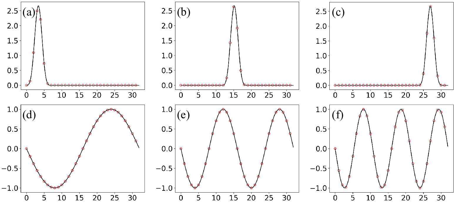
Case II. In this case, we test our algorithm with higher dimension and more change-points. The dimension is set to $p=400$. The length of the time series is set to $N=320$, and suppose there are nine change-points at $\tau_{i}=i\times\frac{N}{10},\ i=1,\dots,9$.

Case III. In this case, the synthetic data are generated based on the GGM model where the covariance matrix or precision matrix changes. The data in each segment are generated from $N(0,\sigma^{2}\boldsymbol{\Sigma}^{(c)}),\ c=1,2$, where $\boldsymbol{\Sigma}^{(c)}=diag(\boldsymbol{\boldsymbol{\Sigma}}^{(c)}_{11},\boldsymbol{\Sigma}^{(c)}_{22})$, $\boldsymbol{\Sigma}^{(c)}_{11}$ and $\boldsymbol{\Sigma}^{(c)}_{22}$ are $20\times 20$ matrices randomly generated by Vine method (Lewandowski et al. 2009) and $\sigma$ is set to 1,2 and 4 in three cases. Other settings are the same as Case I.

First, we provide the detection results of DSSL in detail for Case I when the variance of the noise is set to $\sigma^{2}=0.05^{2}$. The two penalty coefficients are set to $\lambda_{1,0}=0.0028$ and $\lambda_{2}=2.2$. To avoid over-pruning when using $K=\frac{2}{3}\lambda_{2}$, we intentionally replace $n$ with $n-5,\ n-10,\ n-15$ in (13) to get the candidate set of the LCP. Figure 4 shows the 6 representative time series in one run and the fitted ones using the proposed method. Clearly, due to sufficient samples in each subspace, the self-expression is very accurate in all three segments.

Figure 5 shows the estimated coefficients at the final time step for the first three time series of each subspace for illustration. For example, the rows of the first panel represents the coefficients of $\boldsymbol{Y}_{2},\ldots,\boldsymbol{Y}_{40}$ when $\boldsymbol{Y}_{1}$ is used as the response. These coefficients change at two change-points. Only the time series within the same subspace have nonzero coefficients, and each representation is sparse. These coefficients are constant within each segment.

Figure 6(a) shows the selected candidates for the LCP at each time step in one run. Only a very small number of points including the true LCP are selected as the candidates, which can effectively control the computational cost at each step. For instance, at 96 time step, the PELT algorithm only selects $\{91,86,81,69,68,67,66,65,64,63,62,61\}$ as LCP candidates. Figure 6(b) shows the average computation time and confidence interval per step, where the PELT algorithm can save more than 90% of the computation time than the OP algorithm.

Figure 7 shows the mean and confidence interval of the detected LCP at each time step. It can be clearly seen that in most of the cases, the change can be timely detected with only about 10 time steps after the change occurs. Besides, as the observations since the latest change accumulates, the detected location of the LCP becomes more and more accurate. Note that in each replication, the detected LCP often abruptly jumps to the true values shortly after the change occurs. As the detection delay may vary from run to run, the change of the mean detection is not as abrupt as a single run.

In order to further demonstrate the superiority and effectiveness of our model, we compare our DSSL model with DFSL model (Zhang et al. 2020), VCVS model (Kolar and Xing 2012) and GFGL model (Gibberd and Nelson 2017), which are state-of-the-art offline methods. Three offline and two online metrics are used for performance evaluation and comparison. The offline metrics include the precision, recall, and running time. The precision and recall are proposed by Peel and Clauset 2015 to evaluate offline multiple change-point detection algorithms and they are defined as follows:

where $n_{e}$ and $n_{r}$ are the estimated number of change-points and the real number of change-points respectively, $\delta$ is the indicator function, and $s$ is the detection error bound. The precision is then the proportion of estimated change-points that timely detect true change-points. Similarly, recall is the proportion of true change-points that are timely detected. Here we set $s=5$ time steps in the comparison. The two online metrics, i.e., detection delay and running time per step, are used to evaluate the detection timeliness in online applications.

All experiments are replicated 100 times, and the results are shown in Table 1. For precision and recall metrics, the proposed DSSL is superior to other approaches in Case I and Case II. While in Case III, other approaches perform better than DSSL approach. The results show that our DSSL performs perfectly if the data satisfies the SSC assumptions. However, it is inferior to the GGM related methods when only the covariance matrix or precision matrix changes. Since the data are generated based on a different pattern, the BIC criterion may not be the optimal choice in such scenarios. DSSL performs better in Case II than Case I because the change is relatively more significant.

In terms of the running time, GFGL approach is the fastest algorithm and our DSSL approach is slightly slower in Case I and II. However, GFGL is an offline method, and if it is applied online, the whole optimization process has to be repeated at each time step, leading to a much higher overall cost. Note that, in Case II, DFSL approach and VCVS approach are unable to detect change-points due to either insufficient memory or extremely long computational time. In Case III, the DSSL approach has a longer running time because the optimization for LASSO problem is much more time-consuming when data are generated by the GGM model. The maximum number of iterations for solving LASSO is set to 1000 in Case I and II while it is set to 10000 in Case III. The running time can be reduced to one tenth by setting the maximum number of iterations to 1000, at a cost of 10 percent decreasing for precision and recall metrics. As for the detection delay, we only show the results for DSSL, as all other methods are offline. Similarly, DSSL approach performs better in Case II than Case I.

In addition, as the variance of noise increases, the change-points are more difficult to detect with lower precision, lower recall and larger detection delay generally. However, the performance of the proposed DSSL approach does not change a lot in Case III. The reason is that $\sigma^{2}$ in Case III only affects the variation of the data. The correlations among the time series remain the same.

In this subsection, we apply the proposed DSSL to the MSRC-12 Gesture Dataset for gesture tracking (Fothergill et al. 2012). This dataset consists of sequences of human skeletal body part movements and the associated gesture that needs to be recognized by the system. Each sample of the sequences contains 60 variables, which are the three dimensional coordinates of 20 human joints. The body pose is captured at a sample rate of 30Hz with $\pm 2\mathrm{cm}$ accuracy in joint positions. In the MSRC-12 Gesture Dataset, there are 30 subjects and they perform 12 gestures each for ten times. The position of these 20 joints and some snapshots of shoot gesture and throw gesture are shown in Figure 8.

Motion segmentation is often a very critical step for gesture recognition. Here we combine the sequences of two gestures of the same subject together to demonstrate the effectiveness of the proposed method. Specifically, we choose ‘shoot’ and ‘throw’ as the two gestures. In the first segment, the subject stretches his arms out in front of him, holds a pistol in both hands, makes a recoil movement and then returns to the original position. In the second segment, the subject uses his right arm to make an overarm throwing movement and then returns to the original position. For the sake of simplicity, we convert coordinates of the same joint into one distance variable, which represents the distance of the joint from the reference point.

Clearly, some joints share similar trajectories with each other, as these joints move in similar ways, such as the joints on the same arm or the same leg (Figure 9(a)). Some joints have totally different trajectories because they have no correlations. With this regard, we can infer that these joints lie in some subspaces and they can be naturally clustered into different groups. Besides, some joints share similar trajectories in the first segment but have different trajectories in the second segment, such as the joints of the two hands in the combined data. As shown in Figure 9(b), in the first segment, they increase or decrease synchronously, while in the second segment, they increase or decrease in the opposite direction. Therefore, we can apply the proposed method to detect when the gesture changes. We delete the data of the left and right wrist because these data are generally the same with the data of the left and right hand. So in total $p=18$ variables are considered. We only use one historical streaming data to tune the two penalty parameters.

Figure 10 shows the original and fitted variables and the sequentially detected LCPs. The change of the gesture is timely detected only after about 10 time steps. The positions of the joints of head, trunk, legs and feet do not change much in the whole motion sequence. The joints of left arm and right arm play a key role to detect the change-point. The subspaces for each gesture are further identified via the clustering of the coefficient matrix, which are shown in Figure 11. This result is consistent with the actual movement of each joint in these two gestures.

The detection performance of the DSSL approach and other baselines is compared in Table 2. The detection error bound $s$ is set to 10 in the calculation of precision ratio and recall ratio. Similar to the simulation study, the proposed DSSL approach outperforms other benchmarks in the detection accuracy with less running time per step. For all methods, the recall is high while the precision is relatively low, indicating that these two methods sometimes detect other change-points besides the one connecting the two gestures. This is understandable because there may exist some changes in one single gesture. For example, for gesture ‘throw’, the motion can be further divided to three segments due to slight correlation change, i.e., raising a hand, throwing something and putting down this hand. These changes may also be detected, though not often.

References

- Aminikhanghahi and Cook (2017) Aminikhanghahi, S. and D. J. Cook (2017). A survey of methods for time series change point detection. Knowledge and information systems 51(2), 339–367.
- Beck and Teboulle (2009) Beck, A. and M. Teboulle (2009). A fast iterative shrinkage-thresholding algorithm for linear inverse problems. SIAM journal on imaging sciences 2(1), 183–202.
- Bellman (1966) Bellman, R. (1966). Dynamic programming. Science 153(3731), 34–37.
- Dempster (1972) Dempster, A. P. (1972). Covariance selection. Biometrics, 157–175.
- Dhulekar et al. (2015) Dhulekar, N., S. Nambirajan, B. Oztan, and B. Yener (2015). Seizure prediction by graph mining, transfer learning, and transformation learning. In International Workshop on Machine Learning and Data Mining in Pattern Recognition, pp. 32–52. Springer.
- Drton and Perlman (2008) Drton, M. and M. D. Perlman (2008). A sinful approach to gaussian graphical model selection. Journal of Statistical Planning and Inference 138(4), 1179–1200.
- Elhamifar and Vidal (2013) Elhamifar, E. and R. Vidal (2013). Sparse subspace clustering: Algorithm, theory, and applications. IEEE transactions on pattern analysis and machine intelligence 35(11), 2765–2781.
- Fothergill et al. (2012) Fothergill, S., H. Mentis, P. Kohli, and S. Nowozin (2012). Instructing people for training gestural interactive systems. In Proceedings of the SIGCHI Conference on Human Factors in Computing Systems, pp. 1737–1746.
- Foygel and Drton (2010) Foygel, R. and M. Drton (2010). Extended bayesian information criteria for gaussian graphical models. arXiv preprint arXiv:1011.6640.
- Gibberd and Nelson (2017) Gibberd, A. J. and J. D. Nelson (2017). Regularized estimation of piecewise constant gaussian graphical models: The group-fused graphical lasso. Journal of Computational and Graphical Statistics 26(3), 623–634.
- Gómez et al. (2020) Gómez, A. M. E., K. Paynabar, and M. Pacella (2020). Functional directed graphical models and applications in root-cause analysis and diagnosis. Journal of Quality Technology, 1–17.
- Guo et al. (2013) Guo, Y., J. Gao, and F. Li (2013). Spatial subspace clustering for hyperspectral data segmentation. In Conference of The Society of Digital Information and Wireless Communications (SDIWC), Volume 1, pp. 3.
- Haslbeck and Waldorp (2015) Haslbeck, J. and L. J. Waldorp (2015). mgm: Estimating time-varying mixed graphical models in high-dimensional data. arXiv preprint arXiv:1510.06871.
- Jackson et al. (2005) Jackson, B., J. D. Scargle, D. Barnes, S. Arabhi, A. Alt, P. Gioumousis, E. Gwin, P. Sangtrakulcharoen, L. Tan, and T. T. Tsai (2005). An algorithm for optimal partitioning of data on an interval. IEEE Signal Processing Letters 12(2), 105–108.
- Jiao et al. (2018) Jiao, Y., Y. Chen, and Y. Gu (2018). Subspace change-point detection: A new model and solution. IEEE Journal of Selected Topics in Signal Processing 12(6), 1224–1239.
- Killick et al. (2012) Killick, R., P. Fearnhead, and I. A. Eckley (2012). Optimal detection of changepoints with a linear computational cost. Journal of the American Statistical Association 107(500), 1590–1598.
- Kirkland et al. (2015) Kirkland, L.-A., F. Kanfer, and S. Millard (2015). Lasso tuning parameter selection. In Annual Proceedings of the South African Statistical Association Conference, Volume 2015, pp. 49–56. South African Statistical Association (SASA).
- Kitov et al. (2019) Kitov, I., S. Turuntaev, A. Konovalov, A. Stepnov, and V. Pupatenko (2019). Use of waveform cross correlation to reconstruct the aftershock sequence of the august 14, 2016, sakhalin earthquake. Seismic Instruments 55(5), 544–558.
- Kolar and Xing (2011) Kolar, M. and E. Xing (2011). On time varying undirected graphs. In Proceedings of the Fourteenth International Conference on Artificial Intelligence and Statistics, pp. 407–415. JMLR Workshop and Conference Proceedings.
- Kolar and Xing (2012) Kolar, M. and E. P. Xing (2012). Estimating networks with jumps. Electronic journal of statistics 6, 2069.
- Lewandowski et al. (2009) Lewandowski, D., D. Kurowicka, and H. Joe (2009). Generating random correlation matrices based on vines and extended onion method. Journal of multivariate analysis 100(9), 1989–2001.
- Li and Solea (2018) Li, B. and E. Solea (2018). A nonparametric graphical model for functional data with application to brain networks based on fmri. Journal of the American Statistical Association 113(524), 1637–1655.
- Li and Vidal (2015) Li, C.-G. and R. Vidal (2015). Structured sparse subspace clustering: A unified optimization framework. In Proceedings of the IEEE conference on computer vision and pattern recognition, pp. 277–286.
- Li et al. (2017) Li, C.-G., C. You, and R. Vidal (2017). Structured sparse subspace clustering: A joint affinity learning and subspace clustering framework. IEEE Transactions on Image Processing 26(6), 2988–3001.
- Meinshausen and Bühlmann (2006) Meinshausen, N. and P. Bühlmann (2006). High-dimensional graphs and variable selection with the lasso. The annals of statistics 34(3), 1436–1462.
- Nowinski (1981) Nowinski, J. L. (1981). Applications of functional analysis in engineering. International Journal of Engineering Science 19(11), 1377–1390.
- Parsons et al. (2004) Parsons, L., E. Haque, and H. Liu (2004). Subspace clustering for high dimensional data: a review. Acm sigkdd explorations newsletter 6(1), 90–105.
- Peel and Clauset (2015) Peel, L. and A. Clauset (2015). Detecting change points in the large-scale structure of evolving networks. In Twenty-Ninth AAAI Conference on Artificial Intelligence.
- Qiao et al. (2019) Qiao, X., S. Guo, and G. M. James (2019). Functional graphical models. Journal of the American Statistical Association 114(525), 211–222.
- Qiao et al. (2020) Qiao, X., C. Qian, G. M. James, and S. Guo (2020). Doubly functional graphical models in high dimensions. Biometrika 107(2), 415–431.
- Qiu et al. (2016) Qiu, H., F. Han, H. Liu, and B. Caffo (2016). Joint estimation of multiple graphical models from high dimensional time series. Journal of the Royal Statistical Society. Series B, Statistical Methodology 78(2), 487.
- Ren et al. (2015) Ren, Z., T. Sun, C.-H. Zhang, and H. H. Zhou (2015). Asymptotic normality and optimalities in estimation of large gaussian graphical models. The Annals of Statistics 43(3), 991–1026.
- Rothman et al. (2008) Rothman, A. J., P. J. Bickel, E. Levina, and J. Zhu (2008). Sparse permutation invariant covariance estimation. Electronic Journal of Statistics 2, 494–515.
- Scott and Knott (1974) Scott, A. J. and M. Knott (1974). A cluster analysis method for grouping means in the analysis of variance. Biometrics, 507–512.
- Shi et al. (2019) Shi, M., L. Zhang, W. Sun, and X. Song (2019). A fuzzy c-means algorithm guided by attribute correlations and its application in the big data analysis of tunnel boring machine. Knowledge-Based Systems 182, 104859.
- Thatcher et al. (2005) Thatcher, R. W., D. North, and C. Biver (2005). Eeg and intelligence: relations between eeg coherence, eeg phase delay and power. Clinical neurophysiology 116(9), 2129–2141.
- Tibshirani et al. (2005) Tibshirani, R., M. Saunders, S. Rosset, J. Zhu, and K. Knight (2005). Sparsity and smoothness via the fused lasso. Journal of the Royal Statistical Society: Series B (Statistical Methodology) 67(1), 91–108.
- Tierney et al. (2014) Tierney, S., J. Gao, and Y. Guo (2014). Subspace clustering for sequential data. In Proceedings of the IEEE conference on computer vision and pattern recognition, pp. 1019–1026.
- Wang and Xu (2013) Wang, Y.-X. and H. Xu (2013). Noisy sparse subspace clustering. In International Conference on Machine Learning, pp. 89–97. PMLR.
- Wu et al. (2016) Wu, J., Y. Chen, and S. Zhou (2016). Online detection of steady-state operation using a multiple-change-point model and exact bayesian inference. IIE transactions 48(7), 599–613.
- Wu et al. (2019) Wu, J., H. Xu, C. Zhang, and Y. Yuan (2019). A sequential bayesian partitioning approach for online steady-state detection of multivariate systems. IEEE Transactions on Automation Science and Engineering 16(4), 1882–1895.
- Yuan and Lin (2006) Yuan, M. and Y. Lin (2006). Model selection and estimation in regression with grouped variables. Journal of the Royal Statistical Society: Series B (Statistical Methodology) 68(1), 49–67.
- Zhang et al. (2020) Zhang, C., H. Yan, S. Lee, and J. Shi (2020). Dynamic multivariate functional data modeling via sparse subspace learning. Technometrics, 1–14.
- Zhang et al. (2016) Zhang, J., C.-G. Li, H. Zhang, and J. Guo (2016). Low-rank and structured sparse subspace clustering. In 2016 Visual Communications and Image Processing (VCIP), pp. 1–4. IEEE.
- Zhou et al. (2010) Zhou, S., J. Lafferty, and L. Wasserman (2010). Time varying undirected graphs. Machine Learning 80(2), 295–319.
- Zhu et al. (2016) Zhu, H., N. Strawn, and D. B. Dunson (2016). Bayesian graphical models for multivariate functional data.