A Linear Transportation Distance for Pattern Recognition
Abstract
The transportation distance, denoted , has been proposed as a generalisation of Wasserstein distances motivated by the property that it can be applied directly to colour or multi-channelled images, as well as multivariate time-series without normalisation or mass constraints. These distances, as with , are powerful tools in modelling data with spatial or temporal perturbations. However, their computational cost can make them infeasible to apply to even moderate pattern recognition tasks. We propose linear versions of these distances and show that the linear distance significantly improves over the linear distance on signal processing tasks, whilst being several orders of magnitude faster to compute than the distance.
A Linear Transportation Distance for Pattern Recognition
Oliver M. Crook1,2, Mihai Cucuringu3,4, Tim Hurst5, Carola-Bibiane Schönlieb2,4, Matthew Thorpe6, Konstantinos C. Zygalakis4,5
1Department of Biochemistry,
2Department of Applied Mathematics
University of Cambridge,
and Theoretical Physics,
Cambridge, CB2 1GA, UK
University of Cambridge,
Cambridge, CB3 0WA, UK
3Department of Statistics and Mathematical Institute,
4The Alan Turing Institute,
London, NW1 2DB, UK
University of Oxford,
Oxford, OX1 3LB, UK
5School of Mathematics,
6Department of Mathematics,
University of Edinburgh,
University of Manchester,
Edinburgh, EH9 3FD, UK
Manchester, M13 9PL, UK
September 2020
Keywords: Optimal Transport, Linear Embedding, Multi-Channelled Signals.
1 Introduction
Optimal transport has gained in recent popularity because of its ability to model diverse data distributions in the signal and image processing fields [44]. Transportation-based methods have been successfully applied to image analysis, including medical images [6] and facial recognition [45], as well as cosmology [21, 22] and voice recognition. Machine learning and Bayesian statistics have also benefited from transport-based approaches [23, 49, 59, 60, 61, 17].
The popularity of optimal transport is, in part, due to the rise in the number of problems in the experimental and social sciences in which techniques are required to compare signal perturbations across spatial or temporal domains. For example, optimal transport based methods for image registration and warping [38] and image morphing [68] have existed for many years. Transportation techniques provide non-linear methods that jointly model locations and intensities, making transportation based approaches a powerful tool in many problems.
Optimal transport methods, in particular Wasserstein distances, are grounded in a wealth of mathematical theory. Excellent introductions to the advanced mathematical theory of optimal transport are presented in [64, 65], whilst [57] presents the theory with a more applied perspective. Many technical aspects of optimal transport have been explored, including geometric properties [25] and links to evolutionary PDEs [4].
There is much interest in developing efficient methods to compute optimal transport distances and maps. For discrete measures, the optimal transport problem can be solved using linear programming approaches [57]. Since solving a linear programme can be costly, [51] proposed a multi-scale linear programme for efficient computations. Other approaches include flow minimisation techniques [5, 38, 4, 37], and gradient descent approaches [11], as well as multi-scale methods [48, 36]. More recently, Cuturi proposed entropy-regularisation based approaches to compute approximations of the optimal transport problem [14]. These methods have been explored in-depth with many extensions [15, 7, 59, 35, 3, 1, 2, 47]. In order to efficiently compute pairwise optimal transport distances on a large data set, a framework called linear optimal transport was proposed in [67, 46] for the distance. In [67] the linear transportation distance was applied to classification tasks for medical, facial and galaxy images, [46] applied the distance to classification problems in medical, facial, galaxies and bird images, [54] used the framework to generate new images, and [9] used the distance to classify jets in collider data.
Higher-order transportation methods have been proposed in the mathematical analysis literature [31, 62]. In [31] García Trillos and Slepčev proposed the transportation () distance to define discrete-to-continuum convergence of variational problems on point clouds. This was further extended in [62] to a transportation distance (where the notation relates to Sobolev spaces). These transportation distances have several key advantages over the optimal transport distance; these include [62]:
- 1.
They have no need for mass normalisation.
- 2.
They are not restricted to non-negative measures.
- 3.
They more accurately model translations compared to .
- 4.
They can compare signals with different discretisations.
Additionally, the transportation distance can include information on the derivative of the signal. The transportation distances and were proposed in [62] to tackle problems in signal analysis; for example, they were able to apply transportation methods to colour images. They experimentally show that the distance outperforms both distances and distances in classification tasks. However, these higher-order transportation distances require the computation of an optimal transport map (on a higher dimensional space) and this thwarts its application to larger scale pattern recognition tasks, where pairwise distances are needed. In this paper we propose a linear approximation of the distance, which is orders of magnitude faster to compute than the full distance first proposed in [31], whilst retaining some of its favourable properties
Our proposed method can be seen as an extension of the linear Wasserstein framework () [67] to higher order transportation distances. The linearisation is essentially a projection onto the tangent manifold at a given reference point. The geodesic distance (in this case corresponding to the Wasserstein distance) is approximated by the Euclidean distance in the tangent space. Suppose we wish to compare signals/images, then application of optimal transport methods would require computation of distances. In the linear optimal transport framework only distances need to be computed. From here signals/images are then embedded into Euclidean space allowing linear statistical methods to be applied, whilst preserving much of the geometry of the original optimal transport space. In [67] the optimal transport distance of choice is the distance, here we will choose the distance. This choice allows a more general set of unnormalised, not necessarily non-negative, multi-channel signals to modelled, which is not possible in the linear framework.
This manuscript begins by reviewing optimal transport and the and distances. The framework is reviewed in Section 2.3 and we propose our extension to in Section 2.4. We then give an overview on interpolation in the space. A background on numerical methods, more precisely how existing methods for can be adapted to is included in the appendix. In Section 3 we apply our method to classification problems in Australian sign language (Section 3.1), breast cancer histopathology (Section 3.2) and financial time series (Section 3.3). We show that linear () outperforms and that it has similar performance to , but is several orders of magnitude faster. Other applications to synthetic data sets and cell morphometry are given in the appendix.
2 Methods
2.1 Optimal Transport and the Wasserstein Distance
To fix notation, we review the modern Monge-Kantorovich formulation of optimal transport and we refer to the excellent monographs [64, 65, 57, 55] for a thorough exposition. Let and be probability measures on measure spaces and respectively, i.e. . Further, let denote the Borel -algebra on . We define the pushforward of a measure by a function by for all . The inverse of is understood as being in the set theoretic sense, i.e. . We denote by the set of all measures on such that the first marginal is and the second marginal is . To be precise, if and are the canonical projections then and . We call any a transportation plan between and (also called a coupling between and ).
The Kantorovich optimal transport problem is the following variational problem
| (2.1) |
where is a cost function. The minimiser of this problem is called the optimal transport plan and such a minimiser exists when is lower semi-continuous (see, for example [57]). The prototypical example for (when ) is , for this choice of one can define the Wasserstein distance by (see also (2.3) below). When is a metric then (2.1) is also known as the earth mover’s distance.
Now, considering a different formulation, let be a Borel measurable function such that . The Monge optimal transport problem is to solve
| (2.2) |
We call any that satisfies a transport map between and , and the solution to the optimisation problem is called the optimal transport map.
It is worthwhile noting that the formulation of the optimal transport problems in equations (2.1) and (2.2) are not, in general, equivalent. However, if the optimal transport plan can be written in the form then it follows that is an optimal transport map and the two formulations are equivalent, i.e. . A sufficient condition to show that such an optimal transport plan exists is to require that is absolutely continuous with respect to the Lebesgue measure on a compact domain and, in addition, where is strictly convex and superlinear, see [64, Theorem 2.44]. Note that it is easy to find examples where there do not exist transport maps at all. For example, if and .
Let and be the set of Radon measures on with finite moment. For , we define the Wasserstein distance between and in by
| (2.3) |
The Wasserstein space is the metric space . For the case , we can define a distance on by
We briefly review the features that make optimal transport particularly suited to signal and image processing. For an extended survey of these ideas see [44]. Optimal transport is able to provide generative models which can represent diverse data distributions and can capture signal variations as a result of spatial perturbations. Furthermore, there is a well formulated theoretical basis (particularly for ) with interesting geometrical properties, such as existence of minimisers [24, 65], the Riemannian structure of Wasserstein spaces when [4, 53] and characterisation as the weak∗ convergence when is compact [57]. The Riemannian structure allows the characterisation of geodesics (shortest curves) on the space . In addition, there are many methods to compute optimal transport distances, for convenience, we review a selection in the appendix in the context of computing the distance.
2.2 The Transportation Distance
The distance was first introduced in [31] to define a discrete-to-continuum convergence on point clouds. This tool has been been extensively used to study similar statistical problems, e.g. [16, 58, 12, 63, 52, 32, 34, 33, 29, 26, 30, 28, 27], and recently has been shown to be a valuable tool in signal analysis [20, 62]. In this section, we review the definitions and properties of the distance and space.
Given an open and bounded domain we define the space as the set of pairs such that and . We do not make any assumption on the dimension of the range of . Working in this formal and abstract framework of measure theory allows us to formulate our methods for both discrete and continuous signals, simultaneously. Importantly, similarly to the Wasserstein distance but unlike the distance, this framework allows us to compare signals with different discretisations since and need not have the same support. We define the space as
We construct the metric between pairs and as follows:
| (2.4) |
Intuitively, we see that optimal transport plans (that is plans in that achieve the minimum in the above variational problem) strike a balance between matching spatially, i.e. minimising , and matching signal features, i.e. minimising .
Example 2.1.
Let us explain here how images can be represented in . Let be the location of pixels (which usually form a grid over ). We apply by choosing a base measure , this is commonly the uniform measure over , i.e. . An image is then represented by the pair where for RGB images and are the RGB values for the pixel at location . Similarly, for greyscale images one would have where is now the greyscale value for the pixel at location . Of course, one can make different choices for in order to emphasise regions/features of the images. We note that, as we represent the image as a function , then we do not need to assume that the image has unit mass. To apply we would represent the image as a probability measure , and we would therefore have to assume that the image has unit mass (or renormalise). This strong assumption limits the applicability of optimal transport in image processing because it requires ad-hoc renormalisation which may suppress features of the image.
To further understand the distance, we reformulate it as a distance supported on the graphs of functions. Recall that the graph of a function is defined as:
Note that the . We define the following lifted measure on :
where . It is clear that is a well-defined measure on . We can characterise the distance as a distance in the following way [31]:
Thus, we can see that the distance is the distance between the appropriate measures on the graphs of function. This allows us to make the following identification between and through the mapping.
| (2.5) | ||||
| (2.6) |
This connection of the distance and the distance facilitates the transfer of certain Wasserstein properties to the setting; for example, metric properties and existence of minimisers.
It is easy to see that, for any and :
In fact, one can also prove the converse inequalities (up to a constant) and hence can be seen to generalise both weak∗ convergence of measures and convergence of functions (see [31] or Proposition 2.2 below).
The distance can be seen as a special case of optimal transport by observing that coincides with the Kantorovich optimal transport problem between two measures and with cost function .
For reference, we also state a Monge-type formulation of the distance as follows:
| (2.7) |
where is a transportation map. When we write the Monge formulation of optimal transport we are assuming that there is an equivalence between (2.4) and (2.7). This is in general difficult to verify, since the application of Brenier’s theorem does not lead to natural conditions. (Assuming that does not give mass to small sets and both and have a sufficient number of bounded moments then one can apply Brenier’s theorem to where and is defined by (2.1), if is strictly convex; practically this is not reasonable.) However, when and are discrete uniform measures with supports of equal size the Monge formulation (2.7) coincides with the Kantorovich formulation (2.4) (see the proposition below).
Let us recall the identification (2.5-2.6) and the identity . Then, there is a corresponding equivalence between transport maps. That is (assuming all transport maps exist and are unique) let achieve the minimum in (2.7) and achieve the minimum in where is given by (2.2) with . It follows that for -almost every .
Proposition 2.2.
Let be open and bounded and . Then the following holds
Note that not all properties of carry through to . For example is not complete. Indeed, following [31], let and note that , (the Lebesgue measure on ) is a Cauchy sequence in . However, does not converge in and therefore cannot converge in , by part 3 of the above proposition. The completion of can be identified with the set of Young measures, and therefore the space , see [31, Remark 3.6]. We note also that there do not exist geodesics in , however we develop an approach to interpolate in (see section 2.5).
By part 3 in the above proposition inherits some sensitivity to high frequency perturbations from the norm. In contrast, as metricizes the weak* convergence (in compact Euclidean spaces) then is insensitive to high frequency perturbations, see [62, Section 2.2].
We also can deduce that the distance inherits translation sensitivity from . In particular, we can see that distances are insensitive to translations if the supports of the images are disjoint. On the other hand, the distance scales linearly with the size of the translation no matter how large the translation. The distance, although not scaling linearly with translation, is monotonically non-decreasing as a function of translation.
The appears an excellent tool to exploit in pattern recognition problems such as images or times series, however it is as computational demanding as and despite recent advances in computation of optimal transport, e.g. [14], it is still challenging to apply it to large scale problems. In the next section, we review the linear Wasserstein () framework, which was introduced to allow application of optimal transport methods to classification problems [67]. In later sections, we apply the ideas of linear optimal transport to .
2.3 A Linear Framework
The framework was proposed in [67], as a way to apply optimal transport techniques (in particular ) to large scale classification problems for image analysis. Given a set of images, one would need to compute all pairwise distances in order to use methods such as -nearest neighbour classifiers. The framework was developed so that the Wasserstein distance needs to be computed only times. In particular, it is the optimal Wasserstein transport maps between signals that are computed. From here, the images are embedded in Euclidean space therefore allowing linear statistical techniques to be applied [66]. This technique was successfully applied in [6] to detect morphological difference in cancer cells. The technique has been further refined and extended to super-resolution images [45, 46]. In this section, we briefly review the ideas of .
The idea behind the framework is to find the optimal Wasserstein transport maps with respect to one (reference) measure. For simplicity we assume that the Monge problem is equivalent to the Kantorovich problem and, in particular, there exists optimal transport maps. Via an embedding of the transport map into Euclidean space the distance between any two pairs is estimated. More precisely, the framework provides a linear embedding for with respect to a fixed measure [44]. This means the Euclidean distance of the embedded measure and the fixed measure is equal to the distance of the measure and the fixed measure. The Euclidean distance between any two measures is then an approximation to the Wasserstein distance between these measures. These linear embeddings then facilitate the application of standard statistical techniques such as PCA, LDA and K-means. The framework is also invertible and so synthetic, but physically possible signals, can be realised [54].
Let and is our reference measure. Throughout this section, we assume that optimal transport maps exist between and , i.e.
and . If optimal transport maps do not exist then one can still define the distance but there is not a natural way to embed this distance into Euclidean space. We refer to [67, Section 2.3] on how to define the distance using generalised geodesics.
In the setting considered here the Linear Wasserstein Distance, , is defined by [67]:
We observe that is a metric and
Let us assume that has a density with respect to the Lebesgue measure and define
| (2.8) |
Then
| (2.9) |
The map is our linear embedding from the Wasserstein space to Euclidean space. We make the following claims on the embedding.
Proposition 2.3.
Assume is bounded and has a density with respect to the Lebesgue measure. Define where is given by (2.8). Then, the following holds:
- 1.
for any ,
- 2.
,
- 3.
for any ,
- 4.
for any .
Proof.
Since has a density with respect to the Lebesgue measure then transport maps , exist. Since the distance is finite (as is bounded), it follows that which proves (1). (2) follows directly from . (3) was shown already in (2.9). Finally, (4) follows
where we use . ∎
We make a similar definition for discrete measures. If for some then we define
| (2.10) |
Analogously to the Lebesgue density case we have
where we recall that is the Euclidean -norm: . For discrete the map is our linear embedding from the Wasserstein space to Euclidean space.
Proposition 2.4.
Let and assume . Define where is given by (2.10) with . Then, the following holds:
- 1.
for any ,
- 2.
,
- 3.
for any , ,
- 4.
for any .
Proof.
The particular forms of all the measures is enough to guarantee that transport maps all exist. The proof is then analogous to the proof of Proposition 2.3. ∎
Example 2.5.
Let us consider how to generate a new image using the linear embedding. Suppose we have a reference measure with density and a set of measures with optimal transport maps which form the linear embedding through . Given a new point in the linear space we can define a transport map by . We generate a new image by . Note that to generate the new image we only required the reference measure and a new point in the linear space. However, in order to generate the new point it will often be sensible to use the statistics of , for example see [54].
In both the Lebesgue density and uniform discrete case preserves the distance between the reference measure and any given (where for discrete measures is also uniform discrete). Between , one approximates . The next section proposes our extension of the framework to the distance.
2.4 A Linear Framework
In this section, we propose a linear framework. Recall that the distance can be defined as an optimal transport distance between measures supported on the graph of a function. Let be the reference signal and the measure in with support on the graph of . Let , , and define . As in the previous section we will assume that optimal transport maps exist between and , i.e.
Recall that we can write in the form where and is the optimal plan for the Monge problem (2.2) between and with cost . The Linear Transportation Distance () is defined as
Simple manipulations of the distance imply
Following the construction of the embedding in the previous section we go directly to the discrete case (since has support on the graph it cannot have a density with respect to the Lebesgue measure). We assume that for some and we define
| (2.11) | ||||
| (2.12) | ||||
| (2.13) |
Given this definition we can write
The map embeds our signals into Euclidean space. We have the following properties of the embedding (analogous to Propositions 2.3 and 2.4).
Proposition 2.6.
Proof.
As for we have that is exactly when comparing with the reference measure, i.e. . When we are comparing two measures, neither of which are the base measure, then we make the approximation
When then the approximation is only formal. In particular, to derive quantitative bounds between and requires a detailed analysis of the space, including quantitative estimates on curvature. To the authors knowledge there is not yet such a bound between the and distances, although recently [50] have obtained bounds for some perturbations.
Example 2.7.
Let us consider how to generate a new image from the linear space. We recall that colour images can be represented by where are the locations of pixels (which are uniform across ), and represents the RGB values for each pixel. We take a reference image of the same form (in particular ), and note that the embedding (mapping to ) is given by where
To generate a new image we need to invert this mapping. Let . We define . Then are the location of the pixels and are the RGB values in the new image. In the space the new image is represented by where and . This is only well defined if are all unique. If not, then we use barycentric projection (see also Section 2.5), for example if for all then we define to be the empirical average.
2.5 Geodesics and Interpolation
The space is a geodesic space, with easily characterisable geodesics. Letting be the optimal transport plan that minimises the transport problem given by (2.1), we define , where , to be a linear interpolation, as follows:
Then the geodesic in is given by . When there exists transport maps, i.e. then the geodesic can be written where . Let be defined by in (2.8) then since
we see that the projection of the geodesic onto the Euclidean space is the geodesic between the projections. In particular, the geodesic between and in Euclidean space is simply . The same argument holds in the discrete case where is defined by (2.10). Since the projection is invertible (at least in some open neighbourhood of the reference measure) we can map from the Euclidean embedding back to . Notably, this allows one to translate principal eigenvectors in PCA space (of the linear embedding) into modes of variation in , see [67] for more details.
This argument does not directly apply to the space since, by the following remark, the space does not permit geodesics.
Remark 2.8.
Consider the measure and the functions Then the transport between and is from to and from to . The "half way" point would be the measure and the function that takes the value and at , which is not a function.
However, this does not prevent us from interpolating and visualising modes of variation. Indeed, let be the optimal map pushing to , then the map
interpolates between the signals and . In fact, this is the geodesic in ; that is is the geodesic in between and . Although we can invert (defined in (2.11)) in the Wasserstein space, i.e. for all there exists such that (note that this is and not since we are inverting with respect to ) we cannot guarantee that can be written in the form for some . Hence, we cannot in general invert the linear embeddings from back into . Instead we use an approximate inversion. We define where satisfies , and (where we use disintegration of measures) with the latter meaning
In other words, we define the "inverse" map from the linear embedding of back into as the inverse map in and projected onto :
| 1: | |||
| 2: |
The projection onto is done by taking the mean across each fibre in . We note that the second step does not have to be performed in the linear Wasserstein setting. With this definition we are also able to visualise any point in the linear embedding in space.
3 Results
In this section we apply the framework to three real world examples to auslan (Australian sign language), breast cancer histopathology and financial time series. We also include two synthetic examples and a further application to cell morphometry in the appendix. Throughout we will choose .
3.1 Application to Auslan Data
We apply the transportation methodology presented in this manuscript to the Australian Sign language (Auslan) dataset [43]. A native Auslan signer was recorded, using fifth dimension technology gloves, making different signs repeated over a period of weeks. The sign was repeated times at each recording, thus each word was measured times. This means there are a total of signs in the dataset. Each measurement is considered as a multivariate time-series. The measurements taken for each hand are the positions, along with roll, pitch and yaw. In addition, the bend of each of the fingers is recorded. Thus at each frame measurements are observed. We consider the Auslan data as functions , for . We truncate the number of time frames to because little variation was observed past this point. The goal of this task is to classify signs given as input to possible words (labels) as output.
We apply the and frameworks to this dataset. Since can handle multi-channel signals, no additional pre-processing was needed. However, to apply additional pre-processing was required. Firstly, all signals were made positive and then the mean was taken so that there was only a signal channel with positive values. We then normalised so the signal integrated to unity. A linear embedding was obtained as described in previous sections. Once this linear embedding is obtained, we use the 1 nearest neighbour (1NN) algorithm to predict the signs from the linear embedding of the signals. As an assessment of performance we use the macro-F1 score (the harmonic mean of the precision and recall) [39]. We assess performance with a -fold cross-validation framework and repeat times to produce a distribution of scores. In addition, we compare to the standard methodology since for this particular data set, even though costly it is possible to perform the full computation. We also recorded timings for each of the methods.
Table 1 shows that the linear transportation methods are considerably faster than the full transportation methods. Indeed the distance was on the order of magnitude of ten’s of seconds, whilst the full took several hours. Figure 1 demonstrates that our proposed method significantly outperforms the approach (T-test, ) on the Auslan data. There is a loss in classification ability of versus the method, which is unsurprising as the linear transportation method is approximate. However, on the Auslan dataset we observe this difference to be small and this minor improvement comes at computational cost orders of magnitude greater.
| Application | |||
|---|---|---|---|
| Auslan | 12.1 | 13.0 | 91200 |
| Breast Cancer Histopathology | 25407.0 | 2919.8 | |
| Financial Time Series | 39.5 | 192.3 | - |

.
3.2 Application to Breast Cancer Histopathology
In this section, we demonstrate the applicability of to images from breast cancer histopathology. Invasive Ductal Carcinoma is an aggressive and common form of breast cancer and deep learning based approaches have been used to construct classifiers to analyse such data [13, 42]. We analyse these datasets using transportation based approaches. We randomly sample images each from two patients healthy and cancerous, totalling 200 images. Each image is on a pixel grid. To apply to these images we first convert the images to a single intensity channel and renormalise so that the intensities integrate to unity. We apply the approach without any ad-hoc preprocessing, since it can be directly applied to un-normalised multi-channelled images. We compute transport maps in each case using entropy regularised approaches and then linearly embed these images as described in earlier sections. We visualise the linear embeddings using PCA. In addition, we again employ the 1NN classifier using the same framework as in the Auslan application. We report distributions of macro-F1 scores for both and .
From Table 1 we see that the computational cost of the and distances differs significantly more than might be expected. This is due to the distance converging more quickly (and therefore needing fewer iterations than the distance (and conversely in the financial time series example). The distance was not included as a comparison as it was too expensive to compute.
Figure 2 demonstrates clear differences between the embedding and embedding. The cancerous and healthy images separate more obviously in the PCA representation of the embeddings. This is supported when using the 1NN classifier, where a mean macro-F1 score of is reported in the case, whilst for the mean macro-F1 score is representing a greater than improvement. It is clear from the box plots that outperforms (T-test ). Using linear interpolation, we visualise perturbations, in units of standard deviation, in principal component space as synthetic images (Figure 3). The interpolation in the embedding produced by demonstrates localised mass moving from the centre of the image towards the edges. This corresponds to cancer invading the milk ducts in cancerous tissue with open milk ducts in non-cancerous tissue. Linear interpolation in the embedding visualises mass moving from the lower right to the upper left of the plot, there is no physical interpretation for this variation. It is clear that the synthetic images are more interpretable than the synthetic images.


3.3 Application to Financial Time Series
In this section, we consider an application of transportation distances to financial time series data. ore specifically, we use daily close prices for constituents of the SP1500 index, for the period 2 January 2004 - 23 March 2020.
3.3.1 Experimental Setup and Background on Financial Time Series
We only consider instruments (stocks) available throughout the entire history, which amounts to approximately . We use daily log-returns, with the return of instrument , between times and , defined as where denotes the price of instrument at the end of day . On any given day , we consider the matrix of size (where is the vector ), capturing the daily returns for the past days (with fixed throughout the experiments). We refer to as the sliding window, as we vary the time component. The goal is to use and compare various techniques for computing the k-nearest-neighbors of , which we denote by
by pooling together the similarities between the multivariate time series comprising with prior historical time series , where is the future horizon at which we aim to predict. Note that, at any given time , the available history to query for the k-nearest-neighbors of ends at , in order to avoid look forward data snooping. Figure 4 is a schematic diagram of our pipeline process.
Future returns
We consider forward looking returns (referred to as targets) of two different types, and at various horizons. The future return can be the raw returns itself, or various decompositions of it. We let denote the raw return of instrument at time , with future horizon . In our setting, we consider the following future horizons days. One often uses the S&P500 as a proxy for the entire market return. The S&P500 is a stock market index that measures the stock performance of 500 large companies listed on stock exchanges in the US market. The index has a corresponding ETF (Exchange Traded Fund), which can be traded much like any other regular stock (with symbol SPY), and we denote its raw return by . With this in mind, for any instrument , one can then consider its future market-excess return (MR) as . For simplicity, we assume across all instruments , though there are various techniques to infer the individual betas from historical prices [40]. We remark that the main reason for benchmarking our predictions against market-excess returns, as opposed to only raw returns, is essentially to hedge away the market risk and increase the Sharpe Ratio score defined further below.
Estimates of future returns
Once we have identified the k-nearest-neighbor (knn) periods of the current window , the prediction made at time , for a given horizon , is a weighted sum of the corresponding historical future returns, where the weights are inversely proportional to the knn distances. More precisely, if we denote by the vector of forecasts for the future -day raw returns at time , its values are given by
where the weights are given by , normalized such that , where denotes the distance between the current window , and its nearest historical neighbors . Similarly, we compute estimates for the future -day market-excess returns (MR), by pooling together k-nn historical forward looking market-excess returns.
P&L
For performance evaluation, we rely on standard metrics from the finance literature. For a given set of forecasts, the corresponding PnL (Profit and Loss) on day for a given return (shortly chosen to be the raw return or the market excess return ) is defined by
where denotes our forecast for stock on day . Note that the PnL increases if and only if the sign of the forecast agrees with the sign of the future return , and decreases otherwise. The sum is across all the instruments, and is the future return (either raw return (RR) or market-excess return (MR)) of stock on day . We explore different forward looking horizons ). We add a superscript to the PnL calculation to indicate its dependency on horizon and the type of return considered (RR or MR). For instance, in our setting, the -day forward looking market-excess return, computed daily, is given by
Sharpe Ratio
After computing the daily PnL time series for all available days, we capture the risk-adjusted performance by computing the corresponding (annualized) Sharpe Ratio
where the scaling is due to the fact that there are 252 trading days within a calendar year. For simplicity, we apply the same scaling also to the longer horizons , and refer the reader to [8] for an in depth discussion on Sharpe Ratios11 1 The annualized Sharpe Ratio is calculated from daily observations as , where is the average daily PnL return, denotes the risk-free rate, and the standard deviation of the PnL returns. Since the risk-free rate is close to zero over the period of study, we compute the Sharpe Ratio as . and practical considerations arising from the fact that typical forecasts for equity returns are usually serially correlated. We attribute the future -day PnL to each day (leading to overlapping windows), as opposed to maintaining parallel portfolios, and computing their daily total PnL. We are mainly interested in relative performance of the methods, in terms of Sharpe Ratio and PnL, and less on the actual magnitudes of these performance metrics, and their practical considerations.
Average PnL in basis points
In the financial literature, a typical performance measure is the average return per dollar traded, in percentage. For example, one is typically interested in the annualized return of the portfolio. In what follows, we denote by PPT (PnL Per Trade) the average daily PnL per unit of notional (eg., $1). For instance, if at time the available capital is $100, and the cumulative PnL at time (thus after one year) is $10, then the annualized return amounts to 10%. Recalling that 1% amounts to 100 basis points (bpts), an annualized return of 10% translates to approximately PPT = 4 bpts per day (since bpts, which amounts to 10%). Essentially, the PPT is telling us how much would we earn for each $1 traded in the markets (excluding transaction costs and fees). For simplicity, we ignore sizing/liquidity effects and assume that each day, we invest $1 for each of the instruments, which leads us to the following simplified notion of PPT, averaged over the entire trading period comprised of days
Quintile Portfolios
One is often interested in understanding the performance of the forecasts, as a function of their respective magnitudes. To this end, one typically considers only a subset (eg, top % strongest in magnitude forecasts) of the universe of stocks, usually referred to as quantile portfolios in the literature [18]. A quantile-based analysis simply constructs and evaluates portfolios composed of stocks which fall in a specific quantile bucket, or above a quantile threshold. We choose to use upward-contained quintile buckets, which we denote by indicating the quintile rank of each stocks, meaning that stocks with quintile rank correspond to the top fraction of largest-in-magnitude forecasts. The colors in Figures 7 denote the quintile portfolios traded based on the magnitude of the forecasts. For example, the red bars correspond to the full universe of stocks, while the green bars denote the top 40% largest in magnitude forecasts.
3.3.2 Methods Comparison
We compare the prediction performance of , and , and leave out the full due to its prohibitive computational running cost. In addition, we compare to another more classical approach, not relying on transportation distance methodology, given by the simple Pearson correlation between the original time series. More precisely, for each window (matrix of size ), we first standardize the returns in each row (eg, corresponding to each stock), and denote the resulting matrix by . Next, we unwrap each matrix into a vector , and finally compute the pairwise distance between a pair of time windows and , using a correlation-based distance between their corresponding flattened versions: Note that, in light of the pre-processing step that standardized each stock, this corresponds, up to a scaling constant, to the squared Euclidean distance between the corresponding vectors .
Figure 6 shows numerical results comparing the various methods considered. The left column is a heatmap showing the pairwise distance matrix between all days available in history, in the interval 2004 - 2020. We note that clearly highlights the financial crisis occurred in 2008, followed by , and to some extent, , while COR show barely visible signs of this event. The middle columns show a distribution of the pairwise distances, while the right columns show the row sums of the distance matrix. Construing the distance matrix as a network with distance/dissimilarity information, this plot effectively plots the degree of each node (i.e., of each time period corresponding to a sliding window of length 20). The periods of time with the largest dissimilarity degree correspond to the financial crisis in 2008. Note that, for each of visualization, we standardize the degree vector.
Next, we zoom in into the pairwise distance matrix, and show the resulting degrees in Figure 5. After computing the distance matrix, we interpret this as a distance network, and compute the total distance degree of each node, after standardization. In this plot, we are able to recognize many of the major financial market events that have happened over the last two decades: the big financial crisis of 2007-2008, the 2010 Flash crash, the August 2011 markets fall (between May-October 2011), the Chinese market crash from January 2016, the period Oct-Nov 2018 (when the stock market lost more than $2 trillion), August 2019 (a highly volatile month in the global stock markets), and finally, the February 2020 stock market crash triggered by the COVID-19 pandemic. It is interesting to observe that the distance degree corresponding to the COVID-19 pandemic is matched in magnitude only by the 2007-2008 financial crisis. Furthermore, in the top right of Figure 5 we plot the top eigenvalues of the distance matrix, highlighting the usual market mode top eigenvector, with the second eigenvector highly localized on the 2007-2008 financial crisis and the February-March 2020 Covid-19 pandemic period (plots of the top 5 eigenvectors are shown in the Appendix, see Figure 13).


Figure 7 shows portfolio statistics for the various methods, across different target future horizons , for both raw-returns (RR) and market-excess returns (MR). The corresponding cumulative PnL plots across time are given in Figure 8 for future horizons. Here, we fixed the number of nearest neighbors to , and allow the knn search to span back until the start of the available history . When forecasting raw returns (left column in Figure 7), all methods perform rather poorly, with COR and showing the best performance for , while for , clearly outperforms all other methods. This supports the assumption that is better able to model similarities in financial time series.
In the market-excess returns setting, for , all methods return a similar performance in terms of Sharpe Ratio (SR) around 1, except for which has a SR of around 0.5; in terms of PnL, most methods achieve a PPT of 1-3 basis points (bpts). However, for longer horizons, clearly outperforms all other methods, both in terms of Sharpe Ratio and PPT.
| COR | ||||

|

|

|

|
| Raw Returns (RR) | Market-Excess Returns (MR) | |
|
1-day |
||
|
5-day |
||
|
10-day |
| Raw Returns (RR) | Market-Excess Returns (MR) | |
|
1-day |
||
|
5-day |
||
|
10-day |
4 Discussion
We have presented a linear optimal transport distance for use in pattern recognition tasks based on the distance. The distance generalises the Wasserstein distance such that it can be applied to multi-channelled data, for example colour images and multivariate time-series. However, when pairwise distances are needed the computation of the distance can make its routine application in pattern recognition tasks computationally infeasible. We proposed a method to alleviate this problem by extending the framework to the setting and call this the framework. In a dataset of signals, these linear transportation approaches need to only compute transport maps/distances and thus the cost scales linearly in the number of signals. In contrast, if pairwise distance are needed then the cost scales quadratically with the number of signals, which can render the problem infeasible.
We developed the theory required to allow these transportation methods to be applied. Showing the preservation of these transportation distances with respect to a reference signal, as well as showing that the defines a bona fide metric on the space. We additionally showed that the linear transportation methods facilitates a linear embedding of our signals allowing simple statistical methods to be applied to the data.
We compared our methods on Auslan, Breast Cancer Histopathology and Financial times series problems. In each case, the approach significantly outperformed the approach. Furthermore, this came at minimal increased computational cost. Even though often outperformed on this task this improved performance comes at an unreasonable additional computational cost.
Our method still relies on the computation of transport maps and this comes at a cost. We have found entropy regularised methods to perform well but suffer from instability. Fast and stable algorithms which are memory efficient are still needed by the community for reliable computation of transport maps.
Extensions of the framework could be to the manifold setting [19], which would allow computation of the distance on a graph. The barycentre and other transformations have also yet to be explored. Considering has a spatial penalty it could also be combined with other penalty terms for more complex applications, for example one could also include a penalty on derivatives of signals as in the distance, see [62].
Acknowledgements
This work was supported by The Alan Turing Institute under EPSRC grant EP/N510129/1. In addition the authors are grateful for discussions with Elizabeth Soilleux, whose interest in machine learning methods for diagnosing coeliac disease motivated this work, and Dejan Slepčev. OMC is a Wellcome Trust Mathematical Genomics and Medicine student and is grateful for generous funding from the Cambridge school of clinical medicine. MC acknowledges support from the EPSRC grant EP/N510129/1 at The Alan Turing Institute. TDH was supported by The Maxwell Institute Graduate School in Analysis and its Applications, a Centre for Doctoral Training funded by the EPSRC (grant EP/L016508/01), the SFC, Heriot-Watt University and the University of Edinburgh. CBS acknowledges support from the Leverhulme Trust project on ‘Breaking the non-convexity barrier’, the Philip Leverhulme Prize, the Royal Society Wolfson Fellowship, the EPSRC grants EP/S026045/1 and EP/T003553/1, the EPSRC Centre Nr. EP/N014588/1, the Wellcome Innovator Award RG98755, European Union Horizon 2020 research and innovation programmes under the Marie Skodowska-Curie grant agreement No. 777826 (NoMADS) and No. 691070 (CHiPS), the Cantab Capital Institute for the Mathematics of Information and the Alan Turing Institute. MT is grateful for the support of the Cantab Capital Institute for the Mathematics of Information (CCIMI) and Cambridge Image Analysis (CIA) groups at the University of Cambridge, and is supported by the European Research Council under the European Union’s Horizon 2020 research and innovation programme grant agreement No 777826 (NoMADS) and grant agreement No 647812. KCZ was supported by the Alan Turing Institute under the EPSRC grant EP/N510129/1.
References
- [1] B. K. Abid and R. Gower. Stochastic algorithms for entropy-regularized optimal transport problems. In International Conference on Artificial Intelligence and Statistics, pages 1505–1512, 2018.
- [2] M. Z. Alaya, M. Berar, G. Gasso, and A. Rakotomamonjy. Screening sinkhorn algorithm for regularized optimal transport. In Advances in Neural Information Processing Systems, pages 12169–12179, 2019.
- [3] J. Altschuler, J. Niles-Weed, and P. Rigollet. Near-linear time approximation algorithms for optimal transport via sinkhorn iteration. In Advances in Neural Information Processing Systems, pages 1964–1974, 2017.
- [4] L. Ambrosio, N. Gigli, and G. Savaré. Gradient flows: in metric spaces and in the space of probability measures. Springer Science & Business Media, 2008.
- [5] S. Angenent, S. Haker, and A. Tannenbaum. Minimizing flows for the Monge–Kantorovich problem. SIAM J. Math. Anal., 35(1):61–97, 2003.
- [6] S. Basu, S. Kolouri, and G. K. Rohde. Detecting and visualizing cell phenotype differences from microscopy images using transport-based morphometry. Proc. Natl. Acad. Sci., 111(9):3448–3453, 2014.
- [7] J.-D. Benamou, G. Carlier, M. Cuturi, L. Nenna, and G. Peyré. Iterative Bregman projections for regularized transportation problems. SIAM J. Sci. Comput., 37(2):A1111–A1138, 2015.
- [8] E. Benhamou, D. Saltiel, B. Guez, and N. Paris. Testing Sharpe ratio: luck or skill? Preprint arXiv:1905.08042, 2019.
- [9] T. Cai, J. Cheng, K. Craig, and N. Craig. Linearized optimal transport for collider events. Preprint arXiv:2008.08604, 2020.
- [10] G. Carlier, V. Duval, G. Peyré, and B. Schmitzer. Convergence of entropic schemes for optimal transport and gradient flows. SIAM J. Math. Anal., 49(2):1385–1418, 2017.
- [11] R. Chartrand, B. Wohlberg, K. Vixie, and E. Bollt. A gradient descent solution to the Monge–Kantorovich problem. Appl. Math. Sci., 3(22):1071–1080, 2009.
- [12] R. Cristoferi and M. Thorpe. Large data limit for a phase transition model with the -laplacian on point clouds. Eur. J. Appl. Math., pages 1–47, 2018.
- [13] A. Cruz-Roa, A. Basavanhally, F. González, H. Gilmore, M. Feldman, S. Ganesan, N. Shih, J. Tomaszewski, and A. Madabhushi. Automatic detection of invasive ductal carcinoma in whole slide images with convolutional neural networks. In Medical Imaging 2014: Digital Pathology, volume 9041, page 904103. International Society for Optics and Photonics, 2014.
- [14] M. Cuturi. Sinkhorn distances: Lightspeed computation of optimal transport. In Advances in Neural Information Processing Systems, pages 2292–2300, 2013.
- [15] M. Cuturi and A. Doucet. Fast computation of Wasserstein barycenters. In International Conference on Machine Learning, pages 685–693, 2014.
- [16] M. M. Dunlop, D. Slepčev, A. M. Stuart, and M. Thorpe. Large data and zero noise limits of graph-based semi-supervised learning algorithms. Appl. Comp. Harmon. Anal., 2019.
- [17] T. A. El Moselhy and Y. M. Marzouk. Bayesian inference with optimal maps. J. Comput. Phys., 231(23):7815–7850, 2012.
- [18] E. F. Fama and K. R. French. The Cross-Section of Expected Stock Returns. J. Financ., 47(2):427–65, June 1992.
- [19] M. Feldman and R. McCann. Monge’s transport problem on a Riemannian manifold. Trans. Am. Math. Soc., 354(4):1667–1697, 2002.
- [20] J. H. Fitschen, F. Laus, and B. Schmitzer. Optimal transport for manifold-valued images. In Scale Space and Variational Methods in Computer Vision, pages 460–472, 2017.
- [21] U. Frisch, S. Matarrese, R. Mohayaee, and A. Sobolevski. A reconstruction of the initial conditions of the universe by optimal mass transportation. Nature, 417(6886):260, 2002.
- [22] U. Frisch and A. Sobolevskii. Application of optimal transport theory to reconstruction of the early universe. J. Math. Sci, 133(4):1539–1542, 2006.
- [23] C. Frogner, C. Zhang, H. Mobahi, M. Araya, and T. A. Poggio. Learning with a Wasserstein loss. In Advances in Neural Information Processing Systems, pages 2053–2061, 2015.
- [24] W. Gangbo and R. J. McCann. Optimal maps in Monge’s mass transport problem. C. R. Acad. Sci., 321(12):1653–1658, 1995.
- [25] W. Gangbo and R. J. McCann. The geometry of optimal transportation. Acta Math., 177(2):113–161, 1996.
- [26] N. García Trillos. Variational limits of -NN graph based functionals on data clouds. SIAM J. Math. Data Sci., 1(1):93–120, 2019.
- [27] N. García Trillos, M. Gerlach, M. Hein, and D. Slepčev. Error estimates for spectral convergence of the graph Laplacian on random geometric graphs toward the Laplace–Beltrami operator. Found. Comput. Math., pages 1–61, 2019.
- [28] N. García Trillos, Z. Kaplan, T. Samakhoana, and D. Sanz-Alonso. On the consistency of graph-based bayesian semi-supervised learning and the scalability of sampling algorithms. J. Mach. Learn. Res., 21(28):1–47, 2020.
- [29] N. García Trillos and R. Murray. A new analytical approach to consistency and overfitting in regularized empirical risk minimization. Eur. J. Appl. Math., 28(6):886–921, 2017.
- [30] N. García Trillos and D. Sanz-Alonso. Continuum limit of posteriors in graph Bayesian inverse problems. SIAM J. Math. Anal., 50(4):4020–4040, 2018.
- [31] N. García Trillos and D. Slepčev. Continuum limit of total variation on point clouds. Arch. Ration. Mech. Anal., 220(1):193–241, 2016.
- [32] N. García Trillos and D. Slepčev. A variational approach to the consistency of spectral clustering. Appl. Comput. Harmon. Anal., 45(2):239–381, 2018.
- [33] N. García Trillos, D. Slepčev, and J. von Brecht. Estimating perimeter using graph cuts. Adv. Appl. Prob., 49(4):1067–1090, 2017.
- [34] N. García Trillos, D. Slepčev, J. von Brecht, T. Laurent, and X. Bresson. Consistency of Cheeger and ratio graph cuts. J. Mach. Learn. Res., 17(1):6268–6313, 2016.
- [35] A. Genevay, M. Cuturi, G. Peyré, and F. Bach. Stochastic optimization for large-scale optimal transport. In Advances in Neural Information Processing Systems, pages 3440–3448, 2016.
- [36] S. Gerber and M. Maggioni. Multiscale strategies for computing optimal transport. J. Mach. Learn. Res., 18(1):2440–2471, 2017.
- [37] E. Haber, T. Rehman, and A. Tannenbaum. An efficient numerical method for the solution of the optimal mass transfer problem. SIAM J. Sci. Comput., 32(1):197–211, 2010.
- [38] S. Haker, L. Zhu, A. Tannenbaum, and S. Angenent. Optimal mass transport for registration and warping. Int. J. Comput. Vis., 60(3):225–240, 2004.
- [39] H. He and E. A. Garcia. Learning from imbalanced data. IEEE Trans. Knowl. Data. Eng., 21(9):1263–1284, 2008.
- [40] F. Hollstein and M. Prokopczuk. Estimating beta. Journal of Financial and Quantitative Analysis, 51(4):1437–1466, 2016.
- [41] L. Hubert and P. Arabie. Comparing partitions. J. Classif., 2(1):193–218, 1985.
- [42] A. Janowczyk and A. Madabhushi. Deep learning for digital pathology image analysis: A comprehensive tutorial with selected use cases. J. Pathol. Inform., 7, 2016.
- [43] M. W. Kadous. Temporal Classification: Extending the Classification Paradigm to Multivariate Time Series. PhD thesis, University of New South Wales, 2002.
- [44] S. Kolouri, S. Park, M. Thorpe, D. Slepčev, and G. K. Rohde. Optimal mass transport: Signal processing and machine-learning applications. IEEE Signal Process. Mag., 34(4):43–59, 2017.
- [45] S. Kolouri and G. K. Rohde. Transport-based single frame super resolution of very low resolution face images. In Proceedings of the IEEE Conference on Computer Vision and Pattern Recognition, pages 4876–4884, 2015.
- [46] S. Kolouri, A. .B Tosun, J. A. Ozolek, and G. K. Rohde. A continuous linear optimal transport approach for pattern analysis in image datasets. Pattern Recognit., 51:453–462, 2016.
- [47] T. Lin, N. Ho, and M. I. Jordan. On efficient optimal transport: An analysis of greedy and accelerated mirror descent algorithms. Preprint arXiv:1901.06482, 2019.
- [48] Q. Mérigot. A multiscale approach to optimal transport. Comput. Graph. Forum, 30(5):1583–1592, 2011.
- [49] S. Minsker, S. Srivastava, L. Lin, and D. B. Dunson. Robust and scalable Bayes via a median of subset posterior measures. J. Mach. Learn. Res., 18(1):4488–4527, 2017.
- [50] C. Moosmüller and A. Cloninger. Linear optimal transport embedding: Provable fast wasserstein distance computation and classification for nonlinear problems. Preprint arXiv:2008.09165, 2020.
- [51] A. M. Oberman and Y. Ruan. An efficient linear programming method for optimal transportation. Preprint arXiv:1509.03668, 2015.
- [52] B. Osting and T. Reeb. Consistency of Dirichlet partitions. SIAM J. Math. Anal., 49(5):4251–4274, 2017.
- [53] F. Otto. The geometry of dissipative evolution equations: the porous medium equation. Comm. Partial. Diff. Equ., 26:101–174, 2001.
- [54] S. Park and M. Thorpe. Representing and learning high dimensional data with the optimal transport map from a probabilistic viewpoint. In The IEEE Conference on Computer Vision and Pattern Recognition (CVPR), pages 7864–7872, 2018.
- [55] G. Peyré and M. Cuturi. Computational Optimal Transport. Volume 37 of Foundations and Trends in Machine Learning Series. Now Publishers, 2019.
- [56] W. M. Rand. Objective criteria for the evaluation of clustering methods. J. Am. Stat. Assoc., 66(336):846–850, 1971.
- [57] F. Santambrogio. Optimal transport for applied mathematicians. Springer, 2015.
- [58] D. Slepčev and M. Thorpe. Analysis of -laplacian regularization in semisupervised learning. SIAM J. Math. Anal., 51(3):2085–2120, 2019.
- [59] J. Solomon, F. De Goes, G. Peyré, M. Cuturi, A. Butscher, A. Nguyen, T. Du, and L. Guibas. Convolutional Wasserstein distances: Efficient optimal transportation on geometric domains. ACM Trans. Graph., 34(4), 2015.
- [60] S. Srivastava, V. Cevher, Q. Dinh, and D. Dunson. Wasp: Scalable Bayes via barycenters of subset posteriors. In Artif. Intell. Stat., pages 912–920, 2015.
- [61] S. Srivastava, C. Li, and D. B. Dunson. Scalable Bayes via barycenter in Wasserstein space. J. Mach. Learn. Res., 19(1):312–346, 2018.
- [62] M. Thorpe, S. Park, S. Kolouri, G. K. Rohde, and D. Slepčev. A transportation distance for signal analysis. J. Math. Imag. Vis., 59(2):187–210, 2017.
- [63] M. Thorpe and F. Theil. Asymptotic analysis of the Ginzburg-Landau functional on point clouds. Proc. R. Soc. Edinb. A: Math, 149(2):387–427, 2019.
- [64] C. Villani. Topics in Optimal Transportation. American Mathematical Society, 2003.
- [65] C. Villani. Optimal transport: old and new. Springer Science & Business Media, 2008.
- [66] W. Wang, Y. Mo, J. A. Ozolek, and G. K. Rohde. Penalized Fisher discriminant analysis and its application to image-based morphometry. Pattern Recognit. Lett., 32(15):2128–2135, 2011.
- [67] W. Wang, D. Slepčev, S. Basu, J. A. Ozolek, and G. K. Rohde. A linear optimal transportation framework for quantifying and visualizing variations in sets of images. Int. J. Comput. Vis., 101(2):254–269, 2013.
- [68] L. Zhu, Y. Yang, S. Haker, and A. Tannenbaum. An image morphing technique based on optimal mass preserving mapping. IEEE Trans. Imag. Process., 16(6):1481–1495, 2007.
In the appendix we include some additional background on computing the distance and further applications.
Appendix A Computing the Embedding
In this section we review some methods for computing the embedding. In principle, any algorithm that can compute optimal transport distances can be adapted to compute by either interpreting as a Wasserstein distance on the graphs of functions, or as an optimal transport problem with cost . We refer to [55] for a thorough review of computational methods for optimal transport. Here, we review entropy regularised optimal transport and flow minimisation in the setting of . We note that as the Kantorovich problem is a linear program then one can use algorithms such as the simplex or interior-point methods. Although there are multi-scale approaches [51] these are typically not state-of-the-art for high dimensional images/signals and so we omit them from this review.
Once we have obtained optimal maps for each of the transportation problems between and for we can embed into Euclidean space by (2.11-2.13) where . Hence, linear statistical methods can be applied.
A.1 An Entropy Regularisation Approach
We assume two pairs can be written in the form
It was proposed in [14] to consider the entropy regularised problem
| (A.1) |
where is a positive parameter that controls the amount of regularisation, is entropy and defined by
and the minimum in (A.1) is taken over matrices such that the row sums are and the column sums are . When , the results of [10] imply that . Subsequent developments of the entropy regularised approach have appeared in [15, 7]. The measure is referred to as the Sinkhorn distance. It is easy to see that
where is the Gibbs distribution, , and denotes the Kullback-Leibler divergence. The minimisation is taken over the same set as in (A.1) The optimal choice for can be written in the following form:
where are the limits, as , of the sequence
see [7]. The entropy regularisation means the optimal for cannot be written as a transport map. To obtain an approximation to the optimal transport map one can use Barycentric projections as in [51, Section 2.3].
A.2 A Flow Minimisation Approach
Following [38] we derive a flow minimization method for finding the transportation map in . Let be a compact domain with smooth boundary and let and be signals in , where are square-integrable functions. Furthermore, we assume that the measures and admit densities with respect to the Lebesgue measure. Abusing notation we write . The variational problem is finding the diffeomorphic map , which minimises the following energy
| (A.2) | ||||
| (A.3) |
We assume the following polar factorization of . Let and assume the second coordinate is time. We further assume for any fixed , . That is, is a mass preserving rearrangement of . Let be an initial mass preserving map between and , i.e. , for example the Knothe-Rosenblatt coupling [65]. We assume that is invertible in for every and with an abuse of notation we write for this inverse, i.e.
| (A.4) |
We require that . The strategy in [38] is to evolve using a gradient descent step such that it converges to a minimiser of (A.2) satisfying the constraint (A.3) as . We first consider sufficient conditions on in order to guarantee that (A.3) holds for all . The proof of the proposition can be found in [38, Section A.2].
Proposition A.1.
Let be a compact domain with a smooth boundary and . Assume that and have densities with respect to the Lebesgue measure on and with an abuse of notation write and Let be a vector field on satisfying on and on where is the normal to the boundary of . Assume is differentiable and invertible in the sense of (A.4), and satisfies . If, and for all
| (A.5) |
then . Furthermore and where
| (A.6) |
If we restrict ourselves to look for transport maps of the form (A.5-A.6) then we must decide how to choose . Let us define by (A.5) with and by (A.6) with . An obvious criterion is to choose so that decreases quickest over all choices of . To this end we compute the derivative of with respect to .
Lemma A.2.
Proof.
We define
which we can also write as
By a change of variables , and since we have
Differentiating the above we obtain,
We note that hence . ∎
When by the Helmholtz decomposition (in 2D) we can find, for each , two scalar fields and such that (where the dependence on and is supressed) and on where for a function . To find the direction of steepest descent we let and and compute
| (A.8) |
where the third line follows from the divergence theorem and since on , and the fourth line follows from on . It follows that the direction of steepest descent is .
To find , we need to observe that where is rotation clockwise by , i.e. . Taking the divergence we have
Hence, solves the Poisson equation with Dirichlet boundary conditions:
| (A.9) | |||||
| (A.10) |
Appendix B Additional Experiments
To supplement the examples given in the main body of the paper we include three other applications. The first two additional examples are to synthetic 1D and 2D data; the same examples were given in [62]. The final example is an application to cell morphometry which appeared in [6] as an example of the LOT framework.
We repeat Table 1 with the complete set of experiments.
| Application | |||
|---|---|---|---|
| 1-D Synthetic | 1.3 | 0.2 | 90.2 |
| 2-D Synthetic | 7.1 | 16.9 | 707.2 |
| Cell Morphometry | 242.1 | 512.7 | 161080 |
| Auslan | 12.1 | 13.0 | 91200 |
| Breast Cancer Histopathology | 25407.0 | 2919.8 | >345600 |
| Financial Time Series | 39.5 | 192.3 | - |
B.1 One Dimensional Synthetic Signal Processing
We first consider a one dimensional signal processing problem, to test the ability of and to discriminate between different signals. Throughout, we take . We consider the task of discriminating between double hump and a high-frequency perturbation of the hump function: a chirp function. A double hump function is of the form:
| (B.1) |
where denotes the indicator function on the interval and . The constant is chosen such that integrates to unity. A chirp-hump function is given as:
| (B.2) |
where controls the high-frequency perturbation and is chosen so that integrates to unity. To generate our synthetic dataset we proceed as follows, fixing and , we generate from (B.1). We corrupt each signal with standard Gaussian noise to obtain noisy double hump functions. We then obtain two separate classes from the chirp-hump functions by first randomly sampling with equal probability. Each chirp-hump function is then corrupted with standard Gaussian noise. We then obtain functions as chirp-hump functions with proportion having perturbation parameter and proportion having perturbation parameter . All functions are defined on discretized on a uniform gird of length .
To apply to discriminate between these signals we first need to satisfy positivity and mass constraints. Thus, each function is normalised as follows , for a small number . Discrete measures are then defined to be the probability measures with density with respect to the uniform grid on . A reference measure is constructed as an empirical average of all these measures. We then use entropy regularised methods, see [14, 7] or Section A.1 to compute optimal transport plans between and , where ; after which an optimal transport map is computed using barycentric projection. We then embed the measures into Euclidean space as described in Section 2.3. Note that for this linear embedding . This method requires only the computation of transport plans, rather than if all pairwise distance were computed.
The framework can be applied directly without ad-hoc pre-processing and normalisation. The base measure is taken as the uniform measure on . The reference measure is taken to be the base measure and the reference signal is the empirical average of all signals. Optimal plans are computed again using entropy regularised methods from to for . Recall that this requires the computation of the optimal transport plan from to for . The map is then obtained from the plan via barycentric projection. A linear embedding is obtained as detailed in Section 2.4. Note this linear embedding is higher dimensional and .
To assess the discriminating ability of and we apply -means clustering with to the linear embedding to see if we can recover the true underlying classes. Since -means attempts to minimise the within class distance and maximise between class distance, we expect a distance which is able to detect the differences between the classes to have the best performance. We take the clustering returned from the -means algorithm and compare it to the true clustering using the adjusted Rand index (ARI) [56, 41]. An ARI is a score with indicating perfect agreement, indicating the method performs as well as one would expect if random assignment where made and the ARI can be negative if the method is worse than random. We repeat our method times to produce a distribution of scores.
Figure 9 demonstrate the improved performance of using the distance to form a linear embedding of the data. The median ARI using the distance was , whilst the median for using the distance was . The approach outperforms the approach significantly (Kolmogorov-Smirnov (KS) Test, -value less than ). Furthermore, Figure 9 panels (b) and (c) demonstrates that the linear embedding produce much tighter and therefore more interpretable clusters in as compared to .


B.2 Two Dimensional Synthetic Signal Processing
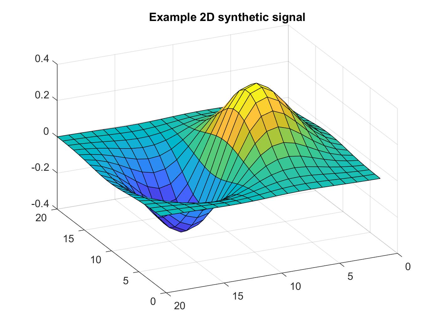
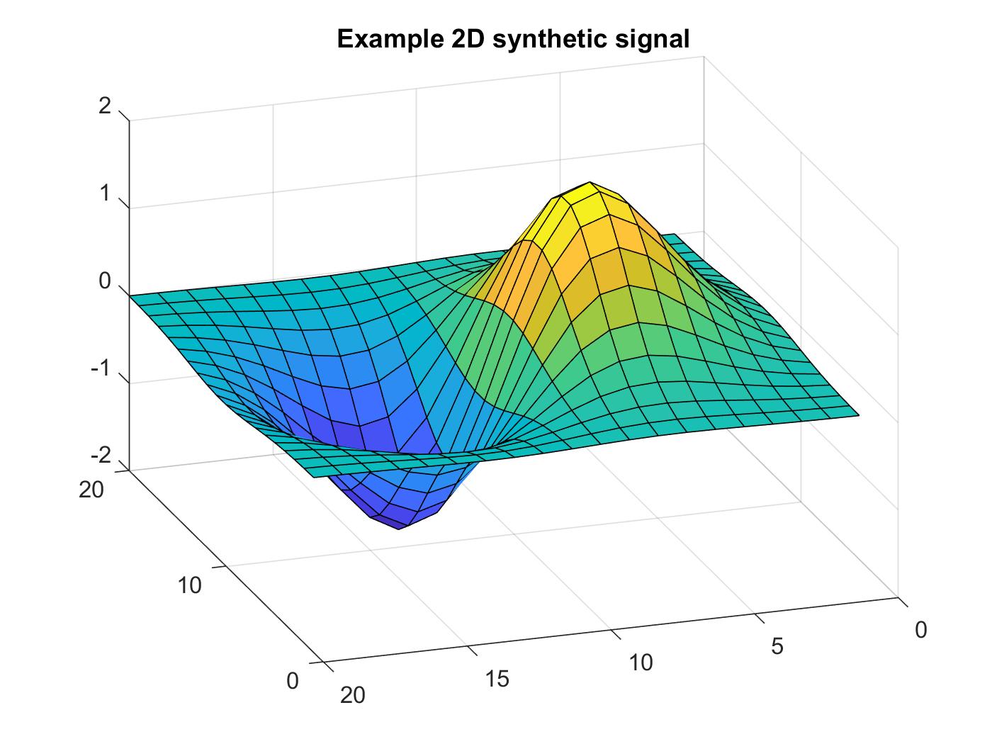
We consider a more challenging synthetic two dimensional signal processing problem. As in the previous section, we take as the exponent of the cost function in both settings. Consider the following class of functions, defined on a grid on :
and
Furthermore, we introduce a perturbation to functions in , by first sampling an integer each with equal probability and then setting for randomly chosen coordinates on the grid, with each coordinate having equal probability of being chosen.
We note that these signals take positive and negative values and thus to apply to this problem we perform normalisation. We add a constant to each (random) function and then ensure that mass still integrates to unity. This ad-hoc normalisation procedure introduces signal compression into the problem causing important features to become suppressed. The distance can be applied without normalisation or pre-processing.
We generate random functions from each class. We then apply both the and methods to the resulting dataset. We performed PCA and -means clustering, with , on the linear embedding to see if we can discriminate between the two classes. As in the previous section, we compare the resultant clustering with ground truth using the ARI. We repeat this process times to obtain a distribution of scores.
Figure 10 show that the embedding outperforms the embedding. The median ARI for the approach is and the median ARI for the approach is . The distance produced significantly better results (KS-test, ) and the PCA plots in Figure 10 demonstrate that the two classes overlap when using but separate when using .


B.3 Application to Cell Morphometry
In this section, we analyse the liver dataset of [6] containing normal and cancerous liver cells. [6] proposed a transportation based morphometry analysis and this facilitated high accuracy classification. Furthermore, the generative nature of optimal transport allowed them to visualise the modes of variation in the dataset, allowing for superior interpretation of the data. Each cell image is defined on a pixel grid with a single intensity channel. Thus both and are applicable.
For consistency we apply flow minimisation techniques to compute the transport maps in each setting [46]. To alleviate numerical issues, as in [46], we apply a Gaussian low-pass filter with standard deviation to smooth the data. We perform mass normalisation so that optimal transport can be applied and these signals are also used for , so that the spatial and intensity features are on the same scale. A linear embedding is obtained from the transport maps.
Once this linear embedding is obtained we use the 1 nearest neighbour (1NN) algorithm to predict normal or cancerous from the linear embedding of the signals. We assess performance with a -fold cross-validation framework; that is, an split between training and testing partitions.
| Raw Returns (RR) | Market-Excess Returns (MR) | |
|
1-day |
||
|
5-day |
||
|
5-day |
||
|
10-day |
Figure 11 shows that on this particular task the and frameworks have similar classification performance when differentiating between cancerous and normal cells. This is unsurprising as these images only have a single intensity channel. We also visualise, in a PCA plot, the embedding showing the variability across the dataset. Figure 11 panel (c) visualises the modes of variation in image space for the first principal components of the data.
B.4 Further Results on the Application to Financial Time Series
We show here additional numerical results for the financial time series applications. Figure 12 shows the PnL curves corresponding the full portfolio of stocks, attained by each of the methods, for the 1,3,5,10-day future horizons, for both the raw returns and market-excess returns. As similarly observed earlier for the top quintile portfolio shown in Figure 8, outperforms all other methods at the longer horizons 3,5,10, especially in the more realistic scenario of using market excess returns (corresponding to a hedged portfolio). Figure 13 shows the top eigenvectors of the distance matrix, which localize on known crises, especially those during 2007-2008 and 2020.
