Optimal convergence rates for elliptic homogenization problems in nondivergence-form: analysis and numerical illustrations

Timo Sprekeler Timo SprekelerUniversity of Oxford, Mathematical Institute, Woodstock Road, Oxford OX2 6GG, UK. Email address: sprekeler@maths.ox.ac.uk and Hung V. Tran Hung V. TranDepartment of Mathematics, University of Wisconsin Madison, Van Vleck hall, 480 Lincoln drive, Madison, WI 53706, USA Email address: hung@math.wisc.edu

Date: August 11, 2026

Abstract.

We study optimal convergence rates in the periodic homogenization of linear elliptic equations of the form $-A(x/\varepsilon):D^{2}u^{\varepsilon}=f$ subject to a homogeneous Dirichlet boundary condition. We show that the optimal rate for the convergence of $u^{\varepsilon}$ to the solution of the corresponding homogenized problem in the $W^{1,p}$ -norm is $\mathcal{O}(\varepsilon)$ . We further obtain optimal gradient and Hessian bounds with correction terms taken into account in the $L^{p}$ -norm. We then provide an explicit $c$ -bad diffusion matrix and use it to perform various numerical experiments, which demonstrate the optimality of the obtained rates.

Key words and phrases:

Homogenization, nondivergence-form elliptic PDE, optimal convergence rates

2010 Mathematics Subject Classification

35B27, 35B40, 35J25

1. Introduction

In this work, we study optimal rates in the periodic homogenization of elliptic equations in nondivergence-form. We consider the linear prototype equation subject to a homogeneous Dirichlet boundary condition, posed on a bounded smooth domain $\Omega\subset\mathbb{R}^{n}$ , i.e., problems of the form

(1.1)

\displaystyle\left\{\begin{aligned} -A\left(\frac{\cdot}{\varepsilon}\right):D^{2}u^{\varepsilon}&=f&&\text{in }\Omega,\\ u^{\varepsilon}&=0&&\text{on }\partial\Omega,\end{aligned}\right.

with a parameter $\varepsilon>0$ (considered to be small), a right-hand side

\displaystyle f\in W^{3,q}(\Omega)\quad\text{for some }q>n,

and a symmetric, $\mathbb{Z}^{n}$ -periodic, uniformly elliptic coefficient function

\displaystyle A\in C^{0,\alpha}(\mathbbm{T}^{n};\mathcal{S}^{n}_{+})\quad\text{for some }\alpha\in(0,1].

Here, $\mathbbm{T}^{n}:=\mathbb{R}^{n}/\mathbb{Z}^{n}$ denotes the flat $n$ -dimensional torus and $\mathcal{S}^{n}_{+}\subset\mathbb{R}^{n\times n}$ the set of symmetric positive definite $n\times n$ matrices. Throughout this work, we denote the unit cell in $\mathbb{R}^{n}$ by

\displaystyle Y:=[0,1]^{n}\subset\mathbb{R}^{n}.

In the theory of periodic homogenization, it is well-known (see e.g., Bensoussan, Lions, Papanicolaou [6], Jikov, Kozlov, Oleinik [26]) that as the parameter $\varepsilon$ tends to zero, the corresponding sequence of solutions $(u^{\varepsilon})_{\varepsilon>0}$ to (1.1) converges uniformly on $\bar{\Omega}$ to the solution $u$ of the homogenized problem

(1.2)

\displaystyle\left\{\begin{aligned} -\bar{A}:D^{2}u&=f&&\text{in }\Omega,\\ u&=0&&\text{on }\partial\Omega.\end{aligned}\right.

Here, the effective coefficient $\bar{A}\in\mathcal{S}^{n}_{+}$ is a constant positive definite matrix, and can be obtained through integration against an invariant measure, that is

\displaystyle\bar{A}:=\int_{Y}Ar

with the invariant measure $r:\mathbb{R}^{n}\rightarrow\mathbb{R}$ being the solution to the periodic problem

\displaystyle-D^{2}:(Ar)=0\quad\text{in }Y,\qquad r\text{ is }Y\text{-periodic},\qquad r>0,\qquad\int_{Y}r=1,

see e.g., Avellaneda, Lin [4], Engquist, Souganidis [13]. The effective coefficient $\bar{A}$ can be equivalently characterized via corrector functions: For $i,j\in\{1,\dots,n\}$ , the $(i,j)$ -th entry $\bar{a}_{ij}$ of $\bar{A}$ is the unique value such that the periodic cell problem

(1.3)

\displaystyle-A:D^{2}v^{ij}=a_{ij}-\bar{a}_{ij}\quad\text{in }Y,\qquad v^{ij}\text{ is }Y\text{-periodic},\qquad\int_{Y}v^{ij}=0

admits a unique solution $v^{ij}:\mathbb{R}^{n}\rightarrow\mathbb{R}$ , called a corrector function.

We are interested in optimal rates for the convergence of the solution $u^{\varepsilon}$ of (1.1) to the solution $u$ of the homogenized problem (1.2) in appropriate function spaces. Optimal rates in $L^{\infty}(\Omega)$ have recently been obtained in Guo, Tran, Yu [22]. With $c_{j}^{kl}\in\mathbb{R}$ , $j,k,l\in\{1,\dots,n\}$ , defined by

(1.4)

\displaystyle c_{j}^{kl}=c_{j}^{kl}(A):=\int_{Y}Ae_{j}\cdot\nabla v^{kl}\,r,

the function $h$ defined by

(1.5)

\displaystyle h:=\sum_{j,k,l=1}^{n}c_{j}^{kl}\partial^{3}_{jkl}u,

and the solution $z$ to the problem

(1.6)

\displaystyle\left\{\begin{aligned} -\bar{A}:D^{2}z&=-h&&\text{in }\Omega,\\ z&=0&&\text{on }\partial\Omega,\end{aligned}\right.

the main result in [22] states the following:

Theorem 1.1 (Theorem 1.2 in [22]).

Assume that $A\in C^{2}(\mathbbm{T}^{n};\mathcal{S}^{n}_{+})$ and $f\in C^{3}(\bar{\Omega})$ . Let $u^{\varepsilon}$ , $u$ and $z$ be the solutions to (1.1), (1.2) and (1.6) respectively. Then we have

\displaystyle\|u^{\varepsilon}-u+2\varepsilon z\|_{L^{\infty}(\Omega)}=\mathcal{O}(\varepsilon^{2}).

In particular, with $h$ given by (1.5), the following assertions hold:

(i)

If $h\equiv 0$ , then $\|u^{\varepsilon}-u\|_{L^{\infty}(\Omega)}=\mathcal{O}(\varepsilon^{2})$ and this rate of convergence is optimal.
(ii)

If $h\not\equiv 0$ , then $\|u^{\varepsilon}-u\|_{L^{\infty}(\Omega)}=\mathcal{O}(\varepsilon)$ and this rate of convergence is optimal.

Remark 1.1.

There is a typo in [22], which uses the opposite sign for the $\mathcal{O}(\varepsilon)$ -term.

Let us recall the $\mathcal{O}$ notation, which we are going to use throughout this paper: For a function $e:(0,\infty)\ni\varepsilon\mapsto e(\varepsilon)\in[0,\infty)$ and an exponent $\gamma\geq 0$ , we write

\displaystyle e(\varepsilon)=\mathcal{O}(\varepsilon^{\gamma})\quad\Longleftrightarrow\quad\exists\,C,\varepsilon_{0}>0:\;e(\varepsilon)\leq C\varepsilon^{\gamma}\quad\forall\varepsilon\in(0,\varepsilon_{0}).

As a consequence of Theorem 1.1, we can classify coefficients $A\in C^{2}(\mathbbm{T}^{n};\mathcal{S}^{n}_{+})$ into those that give optimal rate of convergence $\mathcal{O}(\varepsilon^{2})$ , called the $c$ -good coefficients, and those that give optimal rate of convergence $\mathcal{O}(\varepsilon)$ , called the $c$ -bad coefficients.

Corollary 1.1 ( $c$ -good and $c$ -bad matrices).

Let $A\in C^{2}(\mathbbm{T}^{n};\mathcal{S}^{n}_{+})$ . Then, with $\{c_{j}^{kl}\}_{1\leq j,k,l\leq n}$ given by (1.4), the following assertions hold:

(i)

If $c_{j}^{kl}(A)=0$ for all $j,k,l\in\{1,\dots,n\}$ , then the situation (i) of Theorem 1.1 occurs for any choice of $f$ . We then say $A$ is $c$ -good.
(ii)

If $c_{j}^{kl}(A)\neq 0$ for some $j,k,l\in\{1,\dots,n\}$ , then there exists $f$ such that the situation (ii) of Theorem 1.1 occurs. We then say $A$ is $c$ -bad.

It has further been shown that the set of $c$ -bad matrices is open and dense in $C^{2}(\mathbbm{T}^{n};\mathcal{S}^{n}_{+})$ for dimensions $n\geq 2$ (see Theorem 1.4 in [22]). Therefore, we have generically that the optimal rate is $\mathcal{O}(\varepsilon)$ in $L^{\infty}(\Omega)$ . Related results on convergence rates and error estimates in the periodic homogenization of elliptic equations in divergence-form have been derived by various authors; see e.g., [20, 27, 29, 31, 35] and the references therein.

The objective of this work are the optimal rates in higher-order norms. This question has not been studied yet and it seems that the only available result in higher-order norms is the following $W^{2,p}$ corrector estimate from Capdeboscq, Sprekeler, Süli [8]:

Theorem 1.2 (Theorem 2.8 in [8]).

Assume that $A\in C^{0,\alpha}(\mathbbm{T}^{n};\mathcal{S}^{n}_{+})$ for some $\alpha\in(0,1]$ and $f\in W^{2,p}(\Omega)$ for some $p\in(1,\infty)$ . Further, assume that the solution $u$ to (1.2) satisfies $u\in W^{4,p}(\Omega)\cap W^{2,\infty}(\Omega)$ . Then, with $u^{\varepsilon}$ given by (1.1) and $V=(v^{ij})_{1\leq i,j\leq n}$ given by (1.3), we have

\displaystyle\left\|u^{\varepsilon}-u-\varepsilon^{2}\,V\left(\frac{\cdot}{\varepsilon}\right):D^{2}u\right\|_{W^{2,p}(\Omega)}=\mathcal{O}(\varepsilon^{\frac{1}{p}}).

Note that the standing assumption in [8] is $A\in W^{1,q}(Y)\cap C^{0,\alpha}(\mathbbm{T}^{n};\mathcal{S}^{n}_{+})$ for some $q>n$ , which is useful for the numerical homogenization but not essential for the result of Theorem 1.2. We observe that we cannot expect strong convergence of $u^{\varepsilon}$ to the homogenized solution $u$ in $W^{2,p}(\Omega)$ and that it is necessary to add corrector terms. The optimality of the rate of convergence $\mathcal{O}(\varepsilon^{\frac{1}{p}})$ in Theorem 1.2 has not been discussed yet, which is a gap of knowledge we want to fill. The main contribution of this work is to derive optimal $W^{1,p}(\Omega)$ estimates for $p\in(1,\infty)$ and to provide numerical illustrations.

For the numerical homogenization of linear equations in nondivergence-form, we refer the reader to Capdeboscq, Sprekeler, Süli [8], Froese, Oberman [16], and the references therein. Let us note that the divergence-form case was the focus of active research over the past decades; see e.g., the works [1, 10, 11, 12, 25] by various authors on heterogeneous multiscale methods and multiscale finite element methods.

For some results on fully nonlinear equations of nondivergence-structure, we refer to Camilli, Marchi [7], Kim, Lee [28] for convergence rates and to Gallistl, Sprekeler, Süli [17], Finlay, Oberman [15] for numerical homogenization of Hamilton–Jacobi–Bellman equations.

1.1. Main results

The main result is the following theorem on optimal rates for the convergence of $u^{\varepsilon}$ to the homogenized solution $u$ in $W^{1,p}(\Omega)$ :

Theorem 1.3 ( $W^{1,p}$ estimate and optimal rate).

Assume that $A\in C^{0,\alpha}(\mathbbm{T}^{n};\mathcal{S}^{n}_{+})$ for some $\alpha\in(0,1]$ and $f\in W^{3,q}(\Omega)$ for some $q>n$ . Let $u^{\varepsilon}$ , $u$ and $z$ be the solutions to (1.1), (1.2) and (1.6) respectively. Further, let $V=(v^{ij})_{1\leq i,j\leq n}$ be the matrix of corrector functions given by (1.3). Then, for all $p\in(1,\infty)$ , we have that

\displaystyle\left\|u^{\varepsilon}-u+2\varepsilon z-\varepsilon^{2}\,V\left(\frac{\cdot}{\varepsilon}\right):D^{2}u\right\|_{W^{1,p}(\Omega)}=\mathcal{O}(\varepsilon^{1+\frac{1}{p}}).

In particular, for all $p\in(1,\infty)$ , the sequence $(u^{\varepsilon})_{\varepsilon>0}$ converges to the homogenized solution $u$ strongly in $W^{1,p}(\Omega)$ with the rate

\displaystyle\left\|u^{\varepsilon}-u\right\|_{W^{1,p}(\Omega)}=\mathcal{O}(\varepsilon),

and this rate of convergence $\mathcal{O}(\varepsilon)$ is optimal in general.

Remark 1.2 ( $L^{\infty}$ estimate, gradient estimate and Hessian estimate).

In the situation of Theorem 1.3, the following assertions hold.

(i)

$L^{\infty}$ bound: An inspection of the proof, see (2.14) and (2.6), yields that

(1.7) $\displaystyle\|u^{\varepsilon}-u+2\varepsilon z\|_{L^{\infty}(\Omega)}=\mathcal{O}(\varepsilon^{2}).$

Hence, we recover the result on optimal $L^{\infty}$ rates from Theorem 1.1 under these weaker assumptions on the coefficient $A$ and the right-hand side $f$ .

(ii)

Gradient bound: For all $p\in(1,\infty)$ , we have

(1.8)

\displaystyle\left\|\nabla u^{\varepsilon}-\nabla u+2\varepsilon\nabla z-\varepsilon\sum_{i,j=1}^{n}\nabla v^{ij}\left(\frac{\cdot}{\varepsilon}\right)\partial^{2}_{ij}u\right\|_{L^{p}(\Omega)}=\mathcal{O}(\varepsilon^{1+\frac{1}{p}}).

(iii)

Hessian bound: In view of Theorem 1.2, for all $p\in(1,\infty)$ , there holds

(1.9)

\displaystyle\left\|D^{2}u^{\varepsilon}-D^{2}u-\sum_{i,j=1}^{n}D^{2}v^{ij}\left(\frac{\cdot}{\varepsilon}\right)\partial^{2}_{ij}u\right\|_{L^{p}(\Omega)}=\mathcal{O}(\varepsilon^{\frac{1}{p}}).

An essential role in the proof plays the boundary corrector $\theta^{\varepsilon}$ , which is defined to be the solution to the following problem with oscillations in the boundary data:

(1.10)

\displaystyle\left\{\begin{aligned} -A\left(\frac{\cdot}{\varepsilon}\right):D^{2}\theta^{\varepsilon}&=0&&\text{in }\Omega,\\ \theta^{\varepsilon}&=-V\left(\frac{\cdot}{\varepsilon}\right):D^{2}u&&\text{on }\partial\Omega.\end{aligned}\right.

We then have the following result on the asymptotic behavior of the boundary corrector under the reduced regularity $f\in W^{2,q}(\Omega)$ for some $q>n$ :

Lemma 1.1 (Boundary corrector $W^{1,p}$ bound).

Assume that $A\in C^{0,\alpha}(\mathbbm{T}^{n};\mathcal{S}^{n}_{+})$ for some $\alpha\in(0,1]$ and $f\in W^{2,q}(\Omega)$ for some $q>n$ . Further, let $\theta^{\varepsilon}$ be the solution to the problem (1.10). Then, for all $p\in(1,\infty)$ , we have that

(1.11)

\displaystyle\varepsilon\left\|\theta^{\varepsilon}\right\|_{W^{1,p}(\Omega)}=\mathcal{O}(\varepsilon^{\frac{1}{p}}).

Remark 1.3 (Boundary corrector $W^{2,p}$ bound [8]).

In the situation of Theorem 1.2, there holds

(1.12)

\displaystyle\varepsilon^{2}\left\|\theta^{\varepsilon}\right\|_{W^{2,p}(\Omega)}=\mathcal{O}(\varepsilon^{\frac{1}{p}}).

Let us remark that the estimate (1.11) for $p=2$ has been shown in [2, 32] in the context of divergence-form homogenization by energy estimates. It is worth noting here that we only obtain $W^{1,p}$ and $W^{2,p}$ bounds for the boundary corrector $\theta^{\varepsilon}$ , and we do not study qualitative and quantitative homogenization of (1.10) (for the latter see e.g., [3, 14, 18]).

Another important ingredient in the proof of Theorem 1.3 is the proof of the $\mathcal{O}(\varepsilon)$ rate for the convergence to the homogenized solution in $W^{1,p}(\Omega)$ under the reduced regularity $f\in W^{2,q}(\Omega)$ for some $q>n$ :

Lemma 1.2 ( $W^{1,p}$ convergence rate $\mathcal{O}(\varepsilon)$ ).

Assume that $A\in C^{0,\alpha}(\mathbbm{T}^{n};\mathcal{S}^{n}_{+})$ for some $\alpha\in(0,1]$ and $f\in W^{2,q}(\Omega)$ for some $q>n$ . Let $u^{\varepsilon}$ and $u$ be the solutions to (1.1) and (1.2) respectively. Then, for any $p\in(1,\infty)$ , we have

\displaystyle\|u^{\varepsilon}-u\|_{W^{1,p}(\Omega)}=\mathcal{O}(\varepsilon).

Finally, we demonstrate through numerical experiments that the obtained rates in the previously stated results cannot be improved in general.

Remark 1.4 (Optimality of rates).

The rate $\mathcal{O}(\varepsilon^{2})$ in the $L^{\infty}(\Omega)$ estimate (1.7), the rate $\mathcal{O}(\varepsilon^{1+\frac{1}{p}})$ in the gradient estimate (1.8) and the rate $\mathcal{O}(\varepsilon^{\frac{1}{p}})$ in the Hessian estimate (1.9) are optimal in general. Consequently, also the rates in the boundary corrector estimates (1.11) and (1.12) are optimal in general.

For the numerical illustrations we use an explicit $c$ -bad matrix (recall Corollary 1.1 for the definition of $c$ -bad) and consider a homogenization problem of the form (1.1) with $z\not\equiv 0$ . This is the first direct proof of the existence of a $c$ -bad matrix.

Theorem 1.4 (Explicit $c$ -bad matrix).

The matrix-valued function $A:\mathbb{R}^{2}\rightarrow\mathbb{R}^{2\times 2}$ given by

\displaystyle A(y_{1},y_{2}):=\frac{1}{r(y_{1},y_{2})}\begin{pmatrix}1-\frac{1}{2}\sin(2\pi y_{1})\sin(2\pi y_{2})&0\\ 0&1+\frac{1}{2}\sin(2\pi y_{1})\sin(2\pi y_{2})\end{pmatrix}

with $r:\mathbb{R}^{2}\rightarrow\mathbb{R}$ defined by

\displaystyle r(y_{1},y_{2}):=1+\frac{1}{4}(\cos(2\pi y_{1})-2\sin(2\pi y_{1}))\sin(2\pi y_{2})

is $c$ -bad. More precisely, there holds $c_{1}^{11}=c_{1}^{22}=-\frac{1}{128\pi}$ and $c_{j}^{kl}=0$ otherwise.

We briefly explain the organization of the paper:

1.2. Structure of the paper

In Section 2, we prove the main result, i.e., Theorem 1.3. We start by recalling some uniform estimates from the theory of homogenization in Section 2.1. Thereafter, we prove Lemmata 1.1 and 1.2 in Sections 2.2 and 2.3 respectively, and finally the main theorem in Section 2.4.

In Section 3, we provide numerical illustrations of the convergence rates from Remark 1.2. We start by proving Theorem 1.4 in Section 3.1, providing an explicit $c$ -bad matrix which we use for the numerical experiments. We illustrate the $L^{\infty}$ bound from Remark 1.2 (i) in Section 3.2, the gradient bound from Remark 1.2 (ii) in Section 3.3 and the Hessian bound from Remark 1.2 (iii) in Section 3.4. Numerical illustrations comparing $c$ -bad and $c$ -good problems are provided in Section 3.5.

Finally in Section 4, we discuss some extensions to nonsmooth domains and give some concluding remarks.

2. Proofs of the main results

2.1. Uniform estimates

Uniform estimates are essential in the theory of homogenization and form the basis for the proofs of the main results. The crucial uniform estimate for the proofs is the uniform $C^{1,\alpha}$ estimate from [4] for nondivergence-form homogenization problems.

Lemma 2.1 (Theorem 1 in [4]).

Let $\Omega\subset\mathbb{R}^{n}$ be a bounded $C^{1,\gamma}$ domain. Assume that $A\in C^{0,\alpha}(\mathbbm{T}^{n};\mathcal{S}^{n}_{+})$ for some $\alpha\in(0,1]$ and $f\in L^{q}(\Omega)$ for some $q>n$ . For $\varepsilon>0$ , let $u^{\varepsilon}$ be the solution to the problem (1.1). Then there exists $\nu\in(0,1]$ such that there holds

\displaystyle\|u^{\varepsilon}\|_{C^{1,\nu}(\Omega)}\leq C\|f\|_{L^{q}(\Omega)}

with a constant $C>0$ independent of $\varepsilon$ .

For the proof of Lemma 1.1 it turns out to be useful to transform the problem (1.10) into divergence-form and use the uniform $W^{1,p}$ estimate from [5] for divergence-form homogenization problems.

Lemma 2.2 (Theorem C in [5]).

Let $\Omega\subset\mathbb{R}^{n}$ be a bounded $C^{2,\gamma}$ domain. Assume that $A^{\mathrm{div}}\in C^{0,\alpha}(\mathbbm{T}^{n};\mathbb{R}^{n\times n})$ for some $\alpha\in(0,1]$ is a uniformly elliptic coefficient, $F\in L^{p}(\Omega)$ and $g\in W^{1,p}(\Omega)$ for some $p\in(1,\infty)$ . For $\varepsilon\in(0,1]$ , let $\rho^{\varepsilon}\in W^{1,p}(\Omega)$ be the solution to the problem

\displaystyle\left\{\begin{aligned} -\nabla\cdot\left(A^{\mathrm{div}}\left(\frac{\cdot}{\varepsilon}\right)\nabla\rho^{\varepsilon}\right)&=-\nabla\cdot F&&\text{in }\Omega,\\ \rho^{\varepsilon}&=g&&\text{on }\partial\Omega.\end{aligned}\right.

Then we have the estimate

\displaystyle\|\rho^{\varepsilon}\|_{W^{1,p}(\Omega)}\leq C\left(\|F\|_{L^{p}(\Omega)}+\|g\|_{W^{1,p}(\Omega)}\right)

with a constant $C>0$ independent of $\varepsilon$ .

With the uniform estimates at hand, we can prove the main results. We start with the proof of Lemma 1.1.

2.2. Proof of Lemma 1.1

The main ingredient for the proof of Theorem 1.3 is the asymptotic behavior of the boundary corrector, i.e., the solution $\theta^{\varepsilon}$ to the problem (1.10). We start by proving Lemma 1.1 and it turns out to be useful to transform the problem (1.10) into the divergence-form problem

\displaystyle\left\{\begin{aligned} -\nabla\cdot\left(A^{\mathrm{div}}\left(\frac{\cdot}{\varepsilon}\right)\nabla\theta^{\varepsilon}\right)&=0&&\text{in }\Omega,\\ \theta^{\varepsilon}&=-V\left(\frac{\cdot}{\varepsilon}\right):D^{2}u&&\text{on }\partial\Omega,\end{aligned}\right.

with a coefficient $A^{\mathrm{div}}\in C^{0,\alpha}(\mathbbm{T}^{n};\mathbb{R}^{n\times n})$ for some $\alpha\in(0,1]$ that is uniformly elliptic. Indeed, this is a well-known reduction procedure and can be achieved by multiplication of the equation (1.10) with the invariant measure and addition of a suitable skew-symmetric matrix; see [4].

Proof of Lemma 1.1.

Firstly note that, as $f\in W^{2,q}(\Omega)$ for some $q>n$ , we have $u\in W^{4,q}(\Omega)$ for some $q>n$ and hence also $u\in W^{3,\infty}(\Omega)$ . We further note that, as $A\in C^{0,\alpha}(\mathbb{R}^{n})$ for some $\alpha\in(0,1]$ , we have $V\in C^{2,\alpha}(\mathbb{R}^{n})$ by elliptic regularity theory [19]. We need to show that

(2.1)

\displaystyle\varepsilon\|\theta^{\varepsilon}\|_{W^{1,p}(\Omega)}=\mathcal{O}(\varepsilon^{\frac{1}{p}})

for any $p\in(1,\infty)$ . To this end, we let $\eta\in C_{c}^{\infty}(\mathbb{R}^{n})$ be a cut-off function with the properties $0\leq\eta\leq 1$ ,

\displaystyle\begin{aligned} \eta&\equiv 1&&\text{in}&\left\{x\in\Omega:\mathrm{dist}(x,\partial\Omega)<\frac{\varepsilon}{2}\right\},\\ \eta&\equiv 0&&\text{in}&\left\{x\in\Omega:\mathrm{dist}(x,\partial\Omega)\geq\varepsilon\right\},\end{aligned}

and $\lvert\nabla\eta\rvert=\mathcal{O}(\varepsilon^{-1})$ . Note that this implies that

(2.2)

\displaystyle\left\|\eta\right\|_{L^{p}(\Omega)}+\varepsilon\left\|\nabla\eta\right\|_{L^{p}(\Omega)}=\mathcal{O}(\varepsilon^{\frac{1}{p}})

for any $p\in(1,\infty)$ . We then define the function

\displaystyle\tilde{\theta}^{\varepsilon}:=\theta^{\varepsilon}+\eta\,V\left(\frac{\cdot}{\varepsilon}\right):D^{2}u

and note that it is the solution to the problem

\displaystyle\left\{\begin{aligned} -\nabla\cdot\left(A^{\mathrm{div}}\left(\frac{\cdot}{\varepsilon}\right)\nabla\tilde{\theta}^{\varepsilon}\right)&=-\nabla\cdot F^{\varepsilon}_{1}&&\text{in }\Omega,\\ \tilde{\theta}^{\varepsilon}&=0&&\text{on }\partial\Omega,\end{aligned}\right.

with $F^{\varepsilon}_{1}$ given by

\displaystyle F^{\varepsilon}_{1}:=A^{\mathrm{div}}\left(\frac{\cdot}{\varepsilon}\right)\nabla\left[\eta\,V\left(\frac{\cdot}{\varepsilon}\right):D^{2}u\right].

Using the uniform $W^{1,p}$ estimate from Lemma 2.2, we find that for $\varepsilon\in(0,1]$ and any $p\in(1,\infty)$ , we have

\displaystyle\|\tilde{\theta}^{\varepsilon}\|_{W^{1,p}(\Omega)}\leq C\|F^{\varepsilon}_{1}\|_{L^{p}(\Omega)}\leq C\left\|\eta\,V\left(\frac{\cdot}{\varepsilon}\right):D^{2}u\right\|_{W^{1,p}(\Omega)}.

Therefore, by the triangle inequality, we obtain the estimate

(2.3)

\displaystyle\|\theta^{\varepsilon}\|_{W^{1,p}(\Omega)}\leq C\left\|\eta\,V\left(\frac{\cdot}{\varepsilon}\right):D^{2}u\right\|_{W^{1,p}(\Omega)}.

As we have the bound

\displaystyle\left\|V\left(\frac{\cdot}{\varepsilon}\right):D^{2}u\right\|_{L^{\infty}(\Omega)}+\varepsilon\left\|\nabla\left[V\left(\frac{\cdot}{\varepsilon}\right):D^{2}u\right]\right\|_{L^{\infty}(\Omega)}=\mathcal{O}(1),

and the asymptotic behavior of the cut-off (2.2), we deduce from (2.3) that there holds

\displaystyle\varepsilon\|\theta^{\varepsilon}\|_{W^{1,p}(\Omega)}

\displaystyle\leq C\varepsilon\left(\left\|\nabla\eta\right\|_{L^{p}(\Omega)}+\left(\varepsilon^{-1}+1\right)\left\|\eta\right\|_{L^{p}(\Omega)}\right)=\mathcal{O}(\varepsilon^{\frac{1}{p}}),

which is precisely the claimed bound (2.1). ∎

2.3. Proof of Lemma 1.2

The second ingredient in the proof of Theorem 1.3 is the proof of the $\mathcal{O}(\varepsilon)$ rate for the convergence of $u^{\varepsilon}$ to $u$ under the reduced regularity assumption $f\in W^{2,q}(\Omega)$ for some $q>n$ .

Proof of Lemma 1.2.

We need to show that for any $p\in(1,\infty)$ , there holds

(2.4)

\displaystyle\|u^{\varepsilon}-u\|_{W^{1,p}(\Omega)}=\mathcal{O}(\varepsilon).

With the corrector matrix $V=(v^{ij})_{1\leq i,j\leq n}$ given by (1.3) and the boundary corrector $\theta^{\varepsilon}$ given by (1.10), we let

(2.5)

\displaystyle\phi^{\varepsilon}:=\varepsilon^{2}\left[V\left(\frac{\cdot}{\varepsilon}\right):D^{2}u+\theta^{\varepsilon}\right].

Then we have that the function $u^{\varepsilon}-u-\phi^{\varepsilon}$ satisfies the problem

\displaystyle\left\{\begin{aligned} -A\left(\frac{\cdot}{\varepsilon}\right):D^{2}(u^{\varepsilon}-u-\phi^{\varepsilon})&=\varepsilon F^{\varepsilon}_{2}&&\text{in }\Omega,\\ u^{\varepsilon}-u-\phi^{\varepsilon}&=0&&\text{on }\partial\Omega,\end{aligned}\right.

with $F^{\varepsilon}_{2}$ given by

\displaystyle F^{\varepsilon}_{2}:=\sum_{i,j,k,l=1}^{n}a_{ij}\left(\frac{\cdot}{\varepsilon}\right)\left[2\partial_{i}v^{kl}\left(\frac{\cdot}{\varepsilon}\right)\partial^{3}_{jkl}u+\varepsilon v^{kl}\left(\frac{\cdot}{\varepsilon}\right)\partial^{4}_{ijkl}u\right].

As $f\in W^{2,q}(\Omega)$ for some $q>n$ , we have $u\in W^{4,q}(\Omega)$ and hence $F^{\varepsilon}_{2}$ is uniformly bounded in $L^{q}(\Omega)$ . By the uniform estimate from Lemma 2.1, we have that

\displaystyle\|u^{\varepsilon}-u-\phi^{\varepsilon}\|_{W^{1,\infty}(\Omega)}\leq C\varepsilon\|F^{\varepsilon}_{2}\|_{L^{q}(\Omega)}=\mathcal{O}(\varepsilon).

Finally, by the triangle inequality and Lemma 1.1, we can conclude that

\displaystyle\|u^{\varepsilon}-u\|_{W^{1,p}(\Omega)}\leq\|u^{\varepsilon}-u-\phi^{\varepsilon}\|_{W^{1,p}(\Omega)}+\|\phi^{\varepsilon}\|_{W^{1,p}(\Omega)}=\mathcal{O}(\varepsilon),

which is precisely the claimed convergence rate (2.4). ∎

2.4. Proof of Theorem 1.3

For the proof of the theorem, let us introduce the function $z^{\varepsilon}$ to be the solution to the problem

\displaystyle\left\{\begin{aligned} -A\left(\frac{\cdot}{\varepsilon}\right):D^{2}z^{\varepsilon}&=-h&&\text{in }\Omega,\\ z^{\varepsilon}&=0&&\text{on }\partial\Omega,\end{aligned}\right.

with the function $h$ defined by (1.5). Observe that the function $z$ given by (1.6) is precisely the homogenized solution corresponding to $(z^{\varepsilon})_{\varepsilon>0}$ . We note that as $f\in W^{3,q}(\Omega)$ for some $q>n$ , we have $u\in W^{5,q}(\Omega)$ and hence $h\in W^{2,q}(\Omega)$ . Therefore, we can apply Lemma 1.2 to find that for any $p\in(1,\infty)$ , there holds

(2.6)

\displaystyle\|z^{\varepsilon}-z\|_{W^{1,p}(\Omega)}=\mathcal{O}(\varepsilon).

We further introduce the functions $\chi^{jkl}$ , $j,k,l\in\{1,\dots,n\}$ to be the solutions to the periodic problems

(2.7)

\displaystyle-A:D^{2}\chi^{jkl}=Ae_{j}\cdot\nabla v^{kl}-c_{j}^{kl}\quad\text{in }Y,\quad\chi^{jkl}\text{ is }Y\text{-periodic},\quad\int_{Y}\chi^{jkl}=0.

Note that the functions $\chi^{jkl}$ are well-defined as by definition (1.4) of $c_{j}^{kl}$ , the right-hand side integrated against the invariant measure equals zero, i.e., there holds

\displaystyle\int_{Y}\left(Ae_{j}\cdot\nabla v^{kl}-c_{j}^{kl}\right)r=0.

We also introduce a corresponding boundary corrector $\theta_{\chi}^{\varepsilon}$ to be the solution to the following problem:

(2.8)

\displaystyle\left\{\begin{aligned} -A\left(\frac{\cdot}{\varepsilon}\right):D^{2}\theta_{\chi}^{\varepsilon}&=0&&\text{in }\Omega,\\ \theta_{\chi}^{\varepsilon}&=-\sum_{j,k,l=1}^{n}\chi^{jkl}\left(\frac{\cdot}{\varepsilon}\right)\partial^{3}_{jkl}u&&\text{on }\partial\Omega.\end{aligned}\right.

As we have done for the boundary corrector $\theta^{\varepsilon}$ , we can transform the problem (2.8) into the divergence-form problem

\displaystyle\left\{\begin{aligned} -\nabla\cdot\left(A^{\mathrm{div}}\left(\frac{\cdot}{\varepsilon}\right)\nabla\theta^{\varepsilon}_{\chi}\right)&=0&&\text{in }\Omega,\\ \theta^{\varepsilon}_{\chi}&=-\sum_{j,k,l=1}^{n}\chi^{jkl}\left(\frac{\cdot}{\varepsilon}\right)\partial^{3}_{jkl}u&&\text{on }\partial\Omega,\end{aligned}\right.

with a coefficient $A^{\mathrm{div}}\in C^{0,\alpha}(\mathbbm{T}^{n};\mathbb{R}^{n\times n})$ for some $\alpha\in(0,1]$ that is uniformly elliptic. Let us note that since $u\in W^{5,q}(\Omega)$ for some $q>n$ and $\chi^{jkl}\in C^{2,\beta}(\mathbb{R}^{n})$ for some $\beta\in(0,1]$ by elliptic regularity theory [19], we can apply Lemma 2.2 to find the bound

(2.9)

\displaystyle\varepsilon\|\theta_{\chi}^{\varepsilon}\|_{W^{1,p}(\Omega)}\leq C\varepsilon\sum_{j,k,l=1}^{n}\left\|\chi^{jkl}\left(\frac{\cdot}{\varepsilon}\right)\partial^{3}_{jkl}u\right\|_{W^{1,\infty}(\Omega)}=\mathcal{O}(1)

for any $p\in(1,\infty)$ . Finally, we introduce the function $w^{\varepsilon}$ to be the solution to the problem

(2.10)

\displaystyle\left\{\begin{aligned} -A\left(\frac{\cdot}{\varepsilon}\right):D^{2}w^{\varepsilon}&=\sum_{i,j,k,l=1}^{n}a_{ij}\left(\frac{\cdot}{\varepsilon}\right)\partial_{i}v^{kl}\left(\frac{\cdot}{\varepsilon}\right)\partial^{3}_{jkl}u&&\text{in }\Omega,\\ w^{\varepsilon}&=0&&\text{on }\partial\Omega.\end{aligned}\right.

Now we are in a position to prove the main result.

Proof of Theorem 1.3.

Let $\phi^{\varepsilon}$ be given by (2.5) and $w^{\varepsilon}$ be the solution to (2.10). Then we have that the function $u^{\varepsilon}-u-\phi^{\varepsilon}-2\varepsilon w^{\varepsilon}$ satisfies the problem

\displaystyle\left\{\begin{aligned} -A\left(\frac{\cdot}{\varepsilon}\right):D^{2}(u^{\varepsilon}-u-\phi^{\varepsilon}-2\varepsilon w^{\varepsilon})&=\varepsilon^{2}F^{\varepsilon}_{3}&&\text{in }\Omega,\\ u^{\varepsilon}-u-\phi^{\varepsilon}-2\varepsilon w^{\varepsilon}&=0&&\text{on }\partial\Omega,\end{aligned}\right.

with $F^{\varepsilon}_{3}$ given by

\displaystyle F^{\varepsilon}_{3}:=\sum_{i,j,k,l=1}^{n}a_{ij}\left(\frac{\cdot}{\varepsilon}\right)v^{kl}\left(\frac{\cdot}{\varepsilon}\right)\partial^{4}_{ijkl}u.

As $u\in W^{5,q}(\Omega)$ for $q>n$ , we have that $F^{\varepsilon}_{3}$ is uniformly bounded in $L^{q}(\Omega)$ and hence, by the uniform estimate from Lemma 2.1, we find

(2.11)

\displaystyle\|u^{\varepsilon}-u-\phi^{\varepsilon}-2\varepsilon w^{\varepsilon}\|_{W^{1,\infty}(\Omega)}\leq C\varepsilon^{2}\|F^{\varepsilon}_{3}\|_{L^{q}(\Omega)}=\mathcal{O}(\varepsilon^{2}).

Now, let us define the function

(2.12)

\displaystyle\psi^{\varepsilon}:=\varepsilon^{2}\left[\sum_{j,k,l=1}^{n}\chi^{jkl}\left(\frac{\cdot}{\varepsilon}\right)\partial^{3}_{jkl}u+\theta^{\varepsilon}_{\chi}\right]

with $\chi^{jkl}$ given by (2.7) and $\theta^{\varepsilon}_{\chi}$ given by (2.8). Then we have that the function $w^{\varepsilon}+z^{\varepsilon}-\psi^{\varepsilon}$ satisfies the problem

\displaystyle\left\{\begin{aligned} -A\left(\frac{\cdot}{\varepsilon}\right):D^{2}(w^{\varepsilon}+z^{\varepsilon}-\psi^{\varepsilon})&=\varepsilon F^{\varepsilon}_{4}&&\text{in }\Omega,\\ w^{\varepsilon}+z^{\varepsilon}-\psi^{\varepsilon}&=0&&\text{on }\partial\Omega,\end{aligned}\right.

with $F^{\varepsilon}_{4}$ given by

\displaystyle F^{\varepsilon}_{4}:=\sum_{d,i,j,k,l=1}^{n}a_{ij}\left(\frac{\cdot}{\varepsilon}\right)\left[2\,\partial_{i}\chi^{dkl}\left(\frac{\cdot}{\varepsilon}\right)\partial^{4}_{djkl}u+\varepsilon\chi^{dkl}\left(\frac{\cdot}{\varepsilon}\right)\partial^{5}_{dijkl}u\right].

As $u\in W^{5,q}(\Omega)$ for some $q>n$ , we have that $F^{\varepsilon}_{4}$ is uniformly bounded in $L^{q}(\Omega)$ and hence, by the uniform estimate from Lemma 2.1, we find

(2.13)

\displaystyle\|w^{\varepsilon}+z^{\varepsilon}-\psi^{\varepsilon}\|_{W^{1,\infty}(\Omega)}\leq C\varepsilon\|F^{\varepsilon}_{4}\|_{L^{q}(\Omega)}=\mathcal{O}(\varepsilon).

Combining the bounds (2.11) and (2.13), we obtain

\displaystyle\|u^{\varepsilon}-u+2\varepsilon z^{\varepsilon}-\phi^{\varepsilon}-2\varepsilon\psi^{\varepsilon}\|_{W^{1,\infty}(\Omega)}=\mathcal{O}(\varepsilon^{2}),

and therefore, using the definitions of $\phi^{\varepsilon}$ and $\psi^{\varepsilon}$ from (2.5) and (2.12), we have that

(2.14)

\displaystyle\left\|u^{\varepsilon}-u+2\varepsilon z^{\varepsilon}-\varepsilon^{2}V\left(\frac{\cdot}{\varepsilon}\right):D^{2}u-\varepsilon^{2}\theta^{\varepsilon}-2\varepsilon^{3}\theta^{\varepsilon}_{\chi}\right\|_{W^{1,\infty}(\Omega)}=\mathcal{O}(\varepsilon^{2}).

Finally, using the rate of convergence of $z^{\varepsilon}$ to $z$ given by (2.6), and Lemma 1.1 and the estimate (2.9) to bound the boundary correctors, we conclude that

\displaystyle\left\|u^{\varepsilon}-u+2\varepsilon z-\varepsilon^{2}V\left(\frac{\cdot}{\varepsilon}\right):D^{2}u\right\|_{W^{1,p}(\Omega)}=\mathcal{O}(\varepsilon^{1+\frac{1}{p}})

for any $p\in(1,\infty)$ . ∎

3. Numerical experiments

3.1. An explicit $c$ -bad matrix

In this section, we prove that the matrix-valued function $A:\mathbb{R}^{2}\rightarrow\mathbb{R}^{2\times 2}$ given by

(3.1)

\displaystyle A(y):=\frac{1}{r(y)}\begin{pmatrix}1-\frac{1}{2}\sin(2\pi y_{1})\sin(2\pi y_{2})&0\\ 0&1+\frac{1}{2}\sin(2\pi y_{1})\sin(2\pi y_{2})\end{pmatrix}

with $r:\mathbb{R}^{2}\rightarrow\mathbb{R}$ defined by

(3.2)

\displaystyle r(y):=1+\frac{1}{4}(\cos(2\pi y_{1})-2\sin(2\pi y_{1}))\sin(2\pi y_{2})

is $c$ -bad (recall the notion of $c$ -bad from Corollary 1.1). We observe the following:

Remark 3.1.

The function $r:\mathbb{R}^{2}\rightarrow\mathbb{R}$ given by (3.2) is the invariant measure of $A:\mathbb{R}^{2}\rightarrow\mathbb{R}^{2\times 2}$ given by (3.1). Further note that the problem (1.1) can then be transformed into the divergence-form problem

(3.3)

\displaystyle\left\{\begin{aligned} -\nabla\cdot\left(A^{\mathrm{div}}\left(\frac{\cdot}{\varepsilon}\right)\nabla u^{\varepsilon}\right)&=r\left(\frac{\cdot}{\varepsilon}\right)f&&\text{in }\Omega,\\ u^{\varepsilon}&=0&&\text{on }\partial\Omega,\end{aligned}\right.

with the matrix-valued function $A^{\mathrm{div}}:\mathbb{R}^{n}\rightarrow\mathbb{R}^{n\times n}$ given by

\displaystyle A^{\mathrm{div}}(y):=\begin{pmatrix}1-\frac{1}{2}\sin(2\pi y_{1})\sin(2\pi y_{2})&\frac{1}{2}\cos(2\pi y_{1})\cos(2\pi y_{2})\\ -\frac{1}{2}\cos(2\pi y_{1})\cos(2\pi y_{2})&1+\frac{1}{2}\sin(2\pi y_{1})\sin(2\pi y_{2})\end{pmatrix}.

We can check that $A$ is $c$ -bad by explicitly computing the matrix of corrector functions $V=(v^{ij})_{1\leq i,j\leq 2}$ given by (1.3) and computing the values $\{c_{j}^{kl}\}_{1\leq j,k,l\leq 2}$ given by (1.4).

Proof of Theorem 1.4.

The effective coefficient $\bar{A}\in\mathcal{S}^{2}_{+}$ is given by

(3.4)

\displaystyle\bar{A}=\int_{Y}Ar=\begin{pmatrix}1&0\\ 0&1\end{pmatrix}

and it is a straightforward calculation to check that the matrix of corrector functions $V=(v^{ij})_{1\leq 1,j\leq 2}:\mathbb{R}^{2}\rightarrow\mathbb{R}^{2\times 2}$ is given by

\displaystyle V(y)=-\frac{\sin(2\pi y_{2})}{32\pi^{2}}\begin{pmatrix}\cos(2\pi y_{1})&0\\ 0&\cos(2\pi y_{1})-4\sin(2\pi y_{1})\end{pmatrix}.

Computation of the values $c_{j}^{kl}$ for $j,k,l\in\{1,2\}$ given by (1.4) yields that

\displaystyle c_{1}^{11}

\displaystyle=\int_{Y}ra_{11}\partial_{1}v^{11}=-\frac{1}{128\pi}=\int_{Y}ra_{11}\partial_{1}v^{22}=c_{1}^{22}

for the values of $c_{1}^{11},c_{1}^{22}$ , and that

\displaystyle c_{2}^{11}

\displaystyle=\int_{Y}ra_{22}\partial_{2}v^{11}=0=\int_{Y}ra_{22}\partial_{2}v^{22}=c_{2}^{22}

for the values of $c_{2}^{11},c_{2}^{22}$ . Clearly we have that $c_{j}^{kl}=0$ for any $(j,k,l)\in\{1,2\}^{3}$ with $k\neq l$ . ∎

Let us note that the effective coefficient (3.4) is the identity matrix and hence, the homogenized problem for this $c$ -bad matrix is the Poisson problem

(3.5)

\displaystyle\left\{\begin{aligned} -\Delta u&=f&&\text{in }\Omega,\\ u&=0&&\text{on }\partial\Omega.\end{aligned}\right.

Further, we have that the function $z$ defined by (1.6) is given as the solution to the Poisson problem

(3.6)

\displaystyle\left\{\begin{aligned} -\Delta z&=-\frac{\partial_{1}f}{128\pi}&&\text{in }\Omega,\\ z&=0&&\text{on }\partial\Omega.\end{aligned}\right.

Finally, let us note that the factor $\frac{1}{r}$ in the definition of the $c$ -bad matrix (3.1) is crucial for $c$ -badness. Indeed, removing this factor we obtain a $c$ -good matrix:

Remark 3.2.

The matrix-valued function $A:\mathbb{R}^{2}\rightarrow\mathbb{R}^{2\times 2}$ given by

\displaystyle A(y):=\begin{pmatrix}1-\frac{1}{2}\sin(2\pi y_{1})\sin(2\pi y_{2})&0\\ 0&1+\frac{1}{2}\sin(2\pi y_{1})\sin(2\pi y_{2})\end{pmatrix}

is $c$ -good.

Proof.

The invariant measure is the constant function $r\equiv 1$ and hence, the effective coefficient $\bar{A}\in\mathcal{S}^{2}_{+}$ is given by

\displaystyle\bar{A}=\int_{Y}A=\begin{pmatrix}1&0\\ 0&1\end{pmatrix}.

It is a straightforward calculation to check that the matrix of corrector functions $V=(v^{ij})_{1\leq 1,j\leq 2}:\mathbb{R}^{2}\rightarrow\mathbb{R}^{2\times 2}$ is given by

\displaystyle V(y)=-\frac{\sin(2\pi y_{1})\sin(2\pi y_{2})}{16\pi^{2}}\begin{pmatrix}1&0\\ 0&-1\end{pmatrix}.

Computation of the values $c_{j}^{kl}$ given by (1.4) yields $c_{j}^{kl}=0$ for all $j,k,l\in\{1,2\}$ . ∎

Note that the effective problem for this $c$ -good matrix is again the Poisson problem (3.5), i.e., the homogenized solution coincides with the one from the $c$ -bad problem.

3.2. Numerical illustration of the $L^{\infty}(\Omega)$ rates

We consider the problem (1.1) with the c-bad coefficient matrix $A$ from Theorem 1.4, the domain $\Omega:=(0,1)^{2}$ and the right-hand side

\displaystyle f:\bar{\Omega}\rightarrow\mathbb{R},\quad f(x_{1},x_{2}):=8\pi^{2}\sin(2\pi x_{1})\sin(2\pi x_{2}).

Then, the solution to the homogenized problem (3.5) is given by

\displaystyle u:\bar{\Omega}\rightarrow\mathbb{R},\quad u(x_{1},x_{2})=\sin(2\pi x_{1})\sin(2\pi x_{2}),

and the solution $z$ to the problem (3.6) is given by

\displaystyle z:\bar{\Omega}\rightarrow\mathbb{R},\quad z(x)=\frac{1}{64}\left(\frac{\cosh(2\pi x_{1}-\pi)}{\cosh(\pi)}-\cos(2\pi x_{1})\right)\sin(2\pi x_{2}).

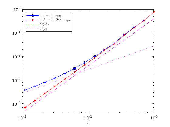
Figure 1 illustrates the estimate (1.7) from Remark 1.2, i.e., for several values of $\varepsilon$ , we plot

(3.7)

\displaystyle E_{0,\infty}^{\varepsilon}:=\|u^{\varepsilon}-u+2\varepsilon z\|_{L^{\infty}(\Omega)}

We approximate the solution $u^{\varepsilon}$ to (1.1) with $\mathbbm{P}_{1}$ finite elements on a fine mesh, based on the natural variational formulation of the divergence-form problem (3.3). We observe the rate $E_{0,\infty}^{\varepsilon}=\mathcal{O}(\varepsilon^{2})$ as $\varepsilon$ tends to zero, as expected from Remark 1.2.

Refer to caption — Figure 1. blue: Plot of $\|u^{\varepsilon}-u\|_{L^{\infty}(\Omega)}$ , red: Plot of $E_{0,\infty}^{\varepsilon}$ (see (3.7)). We observe $\|u^{\varepsilon}-u\|_{L^{\infty}(\Omega)}=\mathcal{O}(\varepsilon)$ and $E_{0,\infty}^{\varepsilon}=\mathcal{O}(\varepsilon^{2})$ as expected from Remark 1.2.

3.3. Numerical illustration of the $W^{1,p}(\Omega)$ rates

We consider the problem (1.1) with the c-bad coefficient matrix $A$ from Theorem 1.4, the domain $\Omega:=(0,1)^{2}$ and the right-hand side

(3.8)

\displaystyle f:\bar{\Omega}\rightarrow\mathbb{R},\quad f(x_{1},x_{2}):=x_{1}(1-x_{1})+x_{2}(1-x_{2}).

Then, the solution of the homogenized problem (3.5) is given by

(3.9)

\displaystyle u:\bar{\Omega}\rightarrow\mathbb{R},\quad u(x_{1},x_{2})=\frac{1}{2}x_{1}(1-x_{1})x_{2}(1-x_{2}).

Figure 2 illustrates the estimate (1.8) from Remark 1.2, i.e., for several values of $\varepsilon$ , we plot

(3.10)

\displaystyle E_{1,p}^{\varepsilon}:=\left\|\nabla u^{\varepsilon}-\nabla u+2\varepsilon\nabla z-\varepsilon\sum_{i,j=1}^{n}\nabla v^{ij}\left(\frac{\cdot}{\varepsilon}\right)\partial^{2}_{ij}u\right\|_{L^{p}(\Omega)}

for the values $p=2,3,4,5$ . We approximate the solution $u^{\varepsilon}$ to (1.1) and the solution $z$ to (3.6) with $\mathbbm{P}_{2}$ finite elements on a fine mesh, based on the natural variational formulation of the divergence-form problems (3.3) and (3.6). We observe the rate $E_{1,p}^{\varepsilon}=\mathcal{O}(\varepsilon^{1+\frac{1}{p}})$ as $\varepsilon$ tends to zero, as expected from Remark 1.2.

3.4. Numerical illustration of the $W^{2,p}(\Omega)$ rates

We consider the problem (1.1) with the c-bad coefficient matrix $A$ from Theorem 1.4, the domain $\Omega:=(0,1)^{2}$ and $f$ given by (3.8). As before, the homogenized solution is given by (3.9). Figure 3 illustrates the estimate (1.9) from Remark 1.2, i.e., for several values of $\varepsilon$ , we plot

(3.11)

\displaystyle E_{2,p}^{\varepsilon}:=\left\|D^{2}u^{\varepsilon}-D^{2}u-\sum_{i,j=1}^{n}D^{2}v^{ij}\left(\frac{\cdot}{\varepsilon}\right)\partial^{2}_{ij}u\right\|_{L^{p}(\Omega)}

for the values $p=2,3,4,5$ . We approximate the solution $u^{\varepsilon}$ to (1.1) with an $H^{2}$ conforming finite element method on a fine mesh, using the HCT element in FreeFem++ [23]. We multiply the equation (1.1) by the invariant measure and use the variational formulation from the framework of linear nondivergence-form equations with Cordes coefficients (see [34]): The solution $u^{\varepsilon}$ to (1.1) is the unique function in $H:=H^{2}(\Omega)\cap H^{1}_{0}(\Omega)$ such that there holds

\displaystyle\int_{\Omega}\frac{\mathrm{tr}\left(\left[rA\right]\left(\frac{\cdot}{\varepsilon}\right)\right)}{\left\lvert\left[rA\right]\left(\frac{\cdot}{\varepsilon}\right)\right\rvert^{2}}\left(-\left[rA\right]\left(\frac{\cdot}{\varepsilon}\right):D^{2}u^{\varepsilon}\right)\Delta v=\int_{\Omega}\frac{\mathrm{tr}\left(\left[rA\right]\left(\frac{\cdot}{\varepsilon}\right)\right)}{\left\lvert\left[rA\right]\left(\frac{\cdot}{\varepsilon}\right)\right\rvert^{2}}\,r\left(\frac{\cdot}{\varepsilon}\right)f\,\Delta v

for any $v\in H$ . We observe the rate $E_{2,p}^{\varepsilon}=\mathcal{O}(\varepsilon^{\frac{1}{p}})$ as $\varepsilon$ tends to zero, as expected from Remark 1.2.

3.5. Comparison of $c$ -bad and $c$ -good problems

We refer to the problem (1.1) with the $c$ -bad coefficient matrix from Theorem 1.4 as the $c$ -bad problem and to the problem (1.1) with the $c$ -good coefficient matrix from Remark 3.2 as the $c$ -good problem. We perform experiments for these two problems with two different choices of right-hand sides, one with known homogenized solution $u$ and one with unknown homogenized solution $u$ . All experiments are performed on the domain $\Omega:=(0,1)^{2}$ .

Let us recall that the homogenized problems corresponding to the $c$ -bad and the $c$ -good problem coincide and that the homogenized solution $u$ is the solution to the Poisson problem (3.5).

3.5.1. $c$ -bad and $c$ -good problems with known (common) homogenized function $u$

We consider the right-hand side $f$ given by (3.8). Then, the solution $u$ of the homogenized problem is known and given by (3.9).

Figure 4 illustrates the $L^{\infty}$ convergence rate $\mathcal{O}(\varepsilon)$ for the $c$ -bad problem and the convergence rate $\mathcal{O}(\varepsilon^{2})$ for the $c$ -good problem. We also illustrate the corrected $L^{\infty}$ bound $E_{0,\infty}^{\varepsilon}=\mathcal{O}(\varepsilon^{2})$ for the $c$ -bad problem. We approximate the solution $u^{\varepsilon}$ to (1.1) and the solution $z$ to (3.6) with $\mathbbm{P}_{2}$ finite elements on a fine mesh, based on the natural variational formulation of the divergence-form problems (3.3) (note $r\equiv 1$ for the $c$ -good problem) and (3.6).

3.5.2. $c$ -bad and $c$ -good problems with unknown (common) homogenized function $u$

We consider the right-hand side $f$ given by

(3.12)

\displaystyle f:\bar{\Omega}\rightarrow\mathbb{R},\quad f(x):=x_{1}^{3}(1-x_{1})^{3}\sin(2\pi(x_{1}-2x_{2})).

Let us note that we do not know the homogenized solution $u$ exactly, we have however that $u\in H^{6}(\Omega)\cap H^{1}_{0}(\Omega)$ as the right-hand side $f\in H^{4}(\Omega)$ satisfies the compatibility conditions $f=0$ and $\partial_{1}^{2}f-\partial_{2}^{2}f=0$ at the corners of the square $(0,1)^{2}=\Omega$ ; see [24].

Figure 5 illustrates the $L^{\infty}$ convergence rate $\mathcal{O}(\varepsilon)$ for the $c$ -bad problem and the convergence rate $\mathcal{O}(\varepsilon^{2})$ for the $c$ -good problem. We also illustrate the corrected $L^{\infty}$ bound $E_{0,\infty}^{\varepsilon}=\mathcal{O}(\varepsilon^{2})$ for the $c$ -bad problem. We approximate the functions $u^{\varepsilon}$ , $u$ and $z$ with $\mathbbm{P}_{2}$ finite elements as before.

4. Extensions and concluding remarks

4.1. Nonsmooth domains

The smoothness assumption on the domain $\Omega$ is used to deduce regularity of $u$ from the regularity assumption on $f$ , and it ensures that the uniform estimates from Section 2.1 hold. We briefly discuss extensions to nonsmooth domains.

4.1.1. $C^{2,\gamma}$ domains

We note that the uniform estimates from Section 2.1 still hold for bounded $C^{2,\gamma}$ domains. Therefore, the result of Theorem 1.3 remains valid with the additional assumption $u\in W^{5,q}(\Omega)$ for some $q>n$ , which has previously been deduced from the regularity of the right-hand side $f$ .

4.1.2. Convex domains

We would like to briefly discuss the case of convex domains. Let $\Omega\subset\mathbb{R}^{n}$ be a bounded convex domain in dimension $n\geq 2$ and assume that the homogenized solution is of regularity $u\in W^{5,q}(\Omega)$ for some $q>n$ . Let us further assume that the coefficient is of regularity $A\in C^{0,\alpha}(\mathbbm{T}^{n};\mathcal{S}^{n}_{+})$ for some $\alpha\in(0,1]$ and satisfies the Cordes condition (which dates back to [9]), i.e., that there exists a constant $\delta\in(0,1]$ such that there holds

(4.1)

\displaystyle\frac{\lvert A\rvert^{2}}{(\mathrm{tr}A)^{2}}\leq\frac{1}{n-1+\delta}\quad\text{in }\mathbb{R}^{n}.

Let us note that the Cordes condition (4.1) is a consequence of uniform ellipticity in two dimensions, i.e., (4.1) holds for any $A\in C^{0,\alpha}(\mathbbm{T}^{2};\mathcal{S}^{2}_{+})$ . Let us also note that Theorem 1.2 holds in this situation for $p=2$ ; see [8].

In the situation described above, there exists a unique solution $u^{\varepsilon}\in H^{2}(\Omega)\cap H^{1}_{0}(\Omega)$ to (1.1) and we have a uniform $H^{2}$ estimate [8, Theorem 2.5]. Therefore, by the Sobolev embedding, we have the uniform $W^{1,p}$ estimate

\displaystyle\|u^{\varepsilon}\|_{W^{1,p}(\Omega)}\leq C\|u^{\varepsilon}\|_{H^{2}(\Omega)}\leq C\|f\|_{L^{2}(\Omega)}

for any $p<2^{*}$ with constants independent of $\varepsilon$ . Here, we write $2^{*}:=\frac{2n}{n-2}$ to denote the critical Sobolev exponent (with the convention that $2^{*}:=\infty$ if $n=2$ ). This uniform estimate replaces the need for the uniform $C^{1,\alpha}$ estimate from Lemma 2.1.

Finally, in order to estimate the boundary corrector, we transformed the problem (1.10) into divergence-form and used that for problems of the form

\displaystyle\left\{\begin{aligned} -\nabla\cdot\left(A^{\mathrm{div}}\left(\frac{\cdot}{\varepsilon}\right)\nabla\rho^{\varepsilon}\right)&=-\nabla\cdot F&&\text{in }\Omega,\\ \rho^{\varepsilon}&=g&&\text{on }\partial\Omega,\end{aligned}\right.

we have (Lemma 2.2) the uniform $W^{1,p}$ estimate

(4.2)

\displaystyle\|\rho^{\varepsilon}\|_{W^{1,p}(\Omega)}\leq C\left(\|F\|_{L^{p}(\Omega)}+\|g\|_{W^{1,p}(\Omega)}\right)

with a constant $C>0$ independent of $\varepsilon$ , assuming that $A^{\mathrm{div}}\in C^{0,\alpha}(\mathbbm{T}^{n};\mathbb{R}^{n\times n})$ for some $\alpha\in(0,1]$ is uniformly elliptic and that $\Omega$ is sufficiently smooth.

Now as $\Omega$ is merely assumed to be convex, we still have (4.2) for $p=2$ by standard arguments and hence, we find that the result of Theorem 1.3 remains true for $p=2$ under the assumptions made in this section. Uniform $W^{1,p}$ estimates for divergence-form problems for a wider range of values $p$ require a more sophisticated approach. With a symmetry assumption on $A^{\mathrm{div}}$ , uniform $W^{1,p}$ estimates for divergence-form problems on Lipschitz domains (recall that bounded convex domains are Lipschitz [21]) have been obtained in [33] for values of $p$ in a certain range around $p=2$ .

4.2. Interpolation

Let us revisit Remark 1.2 and note that the gradient bound (1.8) follows from the $L^{\infty}$ bound (1.7) and the Hessian bound (1.9) via the Gagliardo–Nirenberg interpolation inequality [30] applied to the function

\displaystyle\varphi^{\varepsilon}:=u^{\varepsilon}-u+2\varepsilon z-\varepsilon^{2}\,V\left(\frac{\cdot}{\varepsilon}\right):D^{2}u.

Indeed, let us assume that $\|\varphi^{\varepsilon}\|_{L^{\infty}(\Omega)}=\mathcal{O}(\varepsilon^{2})$ and $\|D^{2}\varphi^{\varepsilon}\|_{L^{p}(\Omega)}=\mathcal{O}(\varepsilon^{\frac{1}{p}})$ for any $p\in(1,\infty)$ . Then the Gagliardo–Nirenberg inequality yields

\displaystyle\|\nabla\varphi^{\varepsilon}\|_{L^{p}(\Omega)}\leq C\left(\|D^{2}\varphi^{\varepsilon}\|_{L^{\frac{p}{2}}(\Omega)}^{\frac{1}{2}}\|\varphi^{\varepsilon}\|_{L^{\infty}(\Omega)}^{\frac{1}{2}}+\|\varphi^{\varepsilon}\|_{L^{\infty}(\Omega)}\right)=\mathcal{O}(\varepsilon^{1+\frac{1}{p}})

for any $p\in(2,\infty)$ . This shows once again that the optimality of the bounds (1.7)–(1.9) is natural. We conclude this paper with a review of the main results.

4.3. Conclusion

In this paper we derived optimal rates of convergence in the periodic homogenization of linear elliptic equations in nondivergence-form. As a result of a $W^{1,p}$ corrector estimate, we obtained that the optimal rate of convergence of $u^{\varepsilon}$ to the homogenized solution in the $W^{1,p}$ -norm is $\mathcal{O}(\varepsilon)$ and also recovered that the optimal convergence rate in the $L^{\infty}$ -norm is $\mathcal{O}(\varepsilon)$ . Moreover, we obtained optimal estimates for the gradient and the Hessian of the solution with correction terms taken into account in $L^{p}$ -norm.

In the final part of the paper, we provided an example of an explicit $c$ -bad matrix and presented several numerical experiments matching the theoretical results and illustrating the optimality of the obtained rates.

Acknowledgements

The authors thank Professor Nam Le (Indiana University Bloomington) for the suggestion of adding Section 4.2. TS is supported by the UK Engineering and Physical Sciences Research Council [EP/L015811/1]. HT is supported in part by NSF grant DMS-1664424 and NSF CAREER grant DMS-1843320.

References

[1] A. Abdulle, W. E, B. Engquist, and E. Vanden-Eijnden. The heterogeneous multiscale method. Acta Numer., 21:1–87, 2012.
[2] G. Allaire and M. Amar. Boundary layer tails in periodic homogenization. ESAIM Control Optim. Calc. Var., 4:209–243, 1999.
[3] S. Armstrong, T. Kuusi, J.-C. Mourrat, and C. Prange. Quantitative analysis of boundary layers in periodic homogenization. Arch. Ration. Mech. Anal., 226(2):695–741, 2017.
[4] M. Avellaneda and F.-H. Lin. Compactness methods in the theory of homogenization. II. Equations in nondivergence form. Comm. Pure Appl. Math., 42(2):139–172, 1989.
[5] M. Avellaneda and F.-H. Lin. $L^{p}$ bounds on singular integrals in homogenization. Comm. Pure Appl. Math., 44(8-9):897–910, 1991.
[6] A. Bensoussan, J.-L. Lions, and G. Papanicolaou. Asymptotic analysis for periodic structures. AMS Chelsea Publishing, Providence, RI, 2011. Corrected reprint of the 1978 original.
[7] F. Camilli and C. Marchi. Rates of convergence in periodic homogenization of fully nonlinear uniformly elliptic PDEs. Nonlinearity, 22(6):1481–1498, 2009.
[8] Y. Capdeboscq, T. Sprekeler, and E. Süli. Finite element approximation of elliptic homogenization problems in nondivergence-form. ESAIM Math. Model. Numer. Anal., 54(4):1221–1257, 2020.
[9] H.O. Cordes. Über die erste Randwertaufgabe bei quasilinearen Differentialgleichungen zweiter Ordnung in mehr als zwei Variablen. Math. Ann., 131:278–312, 1956.
[10] W. E and B. Engquist. The heterogeneous multiscale methods. Commun. Math. Sci., 1(1):87–132, 2003.
[11] Y. Efendiev and T.Y. Hou. Multiscale finite element methods, volume 4 of Surveys and Tutorials in the Applied Mathematical Sciences. Springer, New York, 2009. Theory and applications.
[12] Y.R. Efendiev and X.-H. Wu. Multiscale finite element for problems with highly oscillatory coefficients. Numer. Math., 90(3):459–486, 2002.
[13] B. Engquist and P.E. Souganidis. Asymptotic and numerical homogenization. Acta Numer., 17:147–190, 2008.
[14] W.M. Feldman and I.C. Kim. Continuity and discontinuity of the boundary layer tail. Ann. Sci. Éc. Norm. Supér. (4), 50(4):1017–1064, 2017.
[15] C. Finlay and A.M. Oberman. Approximate homogenization of convex nonlinear elliptic PDEs. Commun. Math. Sci., 16(7):1895–1906, 2018.
[16] B.D. Froese and A.M. Oberman. Numerical averaging of non-divergence structure elliptic operators. Commun. Math. Sci., 7(4):785–804, 2009.
[17] D. Gallistl, T. Sprekeler, and E. Süli. Mixed finite element approximation of periodic Hamilton–Jacobi–Bellman problems with application to numerical homogenization, arXiv:2010.01647 [math.NA].
[18] D. Gérard-Varet and N. Masmoudi. Homogenization and boundary layers. Acta Math., 209(1):133–178, 2012.
[19] D. Gilbarg and N.S. Trudinger. Elliptic partial differential equations of second order. Classics in Mathematics. Springer-Verlag, Berlin, 2001. Reprint of the 1998 edition.
[20] G. Griso. Interior error estimate for periodic homogenization. Anal. Appl. (Singap.), 4(1):61–79, 2006.
[21] P. Grisvard. Elliptic problems in nonsmooth domains, volume 69 of Classics in Applied Mathematics. Society for Industrial and Applied Mathematics (SIAM), Philadelphia, PA, 2011. Reprint of the 1985 original.
[22] X. Guo, H.V. Tran, and Y. Yu. Remarks on optimal rates of convergence in periodic homogenization of linear elliptic equations in non-divergence form. SN Partial Differ. Equ. Appl., 1(15), 2020.
[23] F. Hecht. New development in freefem++. J. Numer. Math., 20(3-4):251–265, 2012.
[24] T. Hell and A. Ostermann. Compatibility conditions for Dirichlet and Neumann problems of Poisson’s equation on a rectangle. J. Math. Anal. Appl., 420(2):1005–1023, 2014.
[25] T.Y. Hou and X.-H. Wu. A multiscale finite element method for elliptic problems in composite materials and porous media. J. Comput. Phys., 134(1):169–189, 1997.
[26] V.V. Jikov, S.M. Kozlov, and O.A. Oleĭnik. Homogenization of differential operators and integral functionals. Springer-Verlag, Berlin, 1994. Translated from the Russian.
[27] C.E. Kenig, F. Lin, and Z. Shen. Convergence rates in $L^{2}$ for elliptic homogenization problems. Arch. Ration. Mech. Anal., 203(3):1009–1036, 2012.
[28] S. Kim and K.-A. Lee. Higher order convergence rates in theory of homogenization: equations of non-divergence form. Arch. Ration. Mech. Anal., 219(3):1273–1304, 2016.
[29] S. Moskow and M. Vogelius. First-order corrections to the homogenised eigenvalues of a periodic composite medium. A convergence proof. Proc. Roy. Soc. Edinburgh Sect. A, 127(6):1263–1299, 1997.
[30] L. Nirenberg. On elliptic partial differential equations. Ann. Scuola Norm. Sup. Pisa Cl. Sci. (3), 13:115–162, 1959.
[31] D. Onofrei and B. Vernescu. Error estimates for periodic homogenization with non-smooth coefficients. Asymptot. Anal., 54(1-2):103–123, 2007.
[32] D. Onofrei and B. Vernescu. Asymptotic analysis of second-order boundary layer correctors. Appl. Anal., 91(6):1097–1110, 2012.
[33] Z. Shen. $W^{1,p}$ estimates for elliptic homogenization problems in nonsmooth domains. Indiana Univ. Math. J., 57(5):2283–2298, 2008.
[34] I. Smears and E. Süli. Discontinuous Galerkin finite element approximation of nondivergence form elliptic equations with Cordès coefficients. SIAM J. Numer. Anal., 51(4):2088–2106, 2013.
[35] T.A. Suslina. Homogenization of the Dirichlet problem for elliptic systems: $L_{2}$ -operator error estimates. Mathematika, 59(2):463–476, 2013.