ContactNets: Learning Discontinuous Contact Dynamics with Smooth, Implicit Representations
Abstract
Common methods for learning robot dynamics assume motion is continuous, causing unrealistic model predictions for systems undergoing discontinuous impact and stiction behavior. In this work, we resolve this conflict with a smooth, implicit encoding of the structure inherent to contact-induced discontinuities. Our method, ContactNets, learns parameterizations of inter-body signed distance and contact-frame Jacobians, a representation that is compatible with many simulation, control, and planning environments for robotics. We furthermore circumvent the need to differentiate through stiff or non-smooth dynamics with a novel loss function inspired by the principles of complementarity and maximum dissipation. Our method can predict realistic impact, non-penetration, and stiction when trained on 60 seconds of real-world data.
1 Introduction
To effectively perform a wide variety of manipulation tasks, intelligent robots must understand not only how they can affect the motion of objects in their environment, but also how objects in their environment interact with one another. While recent accomplishments in planning [1, 2] and control [3], suggest that a model of the robot-environment system’s dynamics is a highly useful formalism for capturing this behavior, producing an accurate model from data is a challenging task for manipulation systems due to the complex behaviors induced by frictional contact.
Many methods for learning a dynamical system attempt to fit a universal function approximator to the system’s equations of motion [4, 5, 6, 7] or inverse dynamics [8], yet often the underlying inductive biases conflict with the the nature of frictional contact. Two ubiquitous representations, fully-connected deep neural networks (DNNs) and Gaussian processes regression with squared-exponential kernels [5, 6, 7], are biased towards similar interpretations of Occam’s razor: the best parameterization (i.e. simplest explanation) is the smoothest interpolator [9] or an infinitely-differentiable regressor [10] of the data. However, physics-based analysis predicts discontinuity [11], non-uniqueness [12], and/or extreme curvature [13] within the equations of motion for systems undergoing frictional contact, and furthermore areas of state-input space crucial to locomotion and manipulation (e.g. footfalls and grasping) are precisely where these irregularities arise. This conflict manifests as poor model predictions even in simple scenarios, as illustrated in Figure 1.


Some works attempt to capture discontinuity with multi-modality [14]. However, unstructured multi-modality is computationally intractable for multi-contact behaviors as the number of modes is extremely large, even in toy systems [15]. DNNs can alternatively be conditioned to generate contact-like behaviors by embedding a differentiable physics simulator directly into their structure [16, 17, 18]. However, differentiating through simulation is numerically challenging if discontinuity is approximated with high-curvature [19], and results from these methods have been limited to simulation and quasi-static real-world interaction with highly-compliant objects. Embedding tactile and force/torque sensors into the robot and/or environment can be effective for learning robot-objects interaction [20, 14], though using such methods to learn object-object interactions would necessitate embedding countless sensors in the robot’s environment.
We present a novel approach to the problem of learning frictional contact behaviors, ContactNets, which eliminates these pervasive difficulties and leads to a well-conditioned problem that is amenable to data-efficient learning. The main contribution of this paper is a reparameterization of the learning problem that effectively uses the inductive bias of DNNs for frictional contact without requiring any contact or force sensing. Inspired by both frictional contact mechanics [21, 22, 13, 11] and implicit representations in deep learning [23], we implicitly parameterize and learn discontinuous contact behaviors as continuous inter-body signed distance functions and contact-frame Jacobians. This representation is equivalent to the parameterization of contact internal to simulators for robotics (e.g. [24, 11, 21, 22, 13]), permitting generation of realistic discontinuous behaviors with efficient numerical optimization. At training time, we circumvent the numerical challenges of differentiating through discontinuous simulators with a novel loss function inspired by the principles of complementarity and maximum dissipation. We evaluate our method on a real-world, dynamic, 3D frictional contact scenario and compare its performance to an unstructured baseline.
2 Background
A robotic manipulator interacting with rigid objects and environment can be modeled with inputs (e.g. motor torques) and states , where represents the robot’s configuration and object poses and represents velocities. The discrete-time dynamics of this system can be formulated as a generalization of Newton’s second law emerging from Lagrangian mechanics:
| (1) |
represents inertial quantities, and is the net generalized impulse over the timestep11 1 We use the letter to denote behaviors emergent from contact forces for notational clarity, but note that is the net impulse over the timestep, i.e. .. Configurations are updated via integration of the velocity22 2 For 3D systems, and often use different coordinates (e.g. quaternions and angular velocities) which obey , where is a Jacobian. (2) and (4) become and ., e.g.
| (2) |
For a system experiencing up to contact interactions, can be decomposed as
| (3) |
aggregates smooth, non-contact impulses which emerge from potential (e.g. gravitational), gyroscopic, and input impulses; and for each , is the net impulse due to the th contact. Here, is the configuration-dependent contact Jacobian which maps generalized velocities into Euclidean velocities in the th contact frame normal () and tangential () directions. are the contact-frame normal impulses , which resist interpenetration; and frictional impulses , which resist sliding motion between the contacting surfaces.
The underlying mathematics in simulators for rigid robots and environments (e.g. MuJoCo [13], Bullet [11], Drake [24], and others [21, 22]) stray very little from the structure in (1)–(3), and are primarily differentiated in their methodology for calculating the contact impulses . However, many models approximate the same two essential characterizations of contact behavior:
- •
Normal complementarity: The signed distance function captures contact geometry as inter-body distances. Because bodies cannot interpenetrate and normal forces only push bodies apart when they touch, for each contact ,
(4) - •
3 Related work
A large body of research ([1, 2, 14, 26, 15, 17, 18, 20] and others) in learning and robotics has recognized many challenges in identifying and controlling frictional contact behaviors. Even smooth contact-induced motion is complex due to partial observability, multi-modality, and stochasticity. Several recent works focus on objects sliding on flat surfaces via pushing; Zhou et al. 2016 learn a set-valued representation of frictional forces via convex optimization and Bauza and Rodriguez 2017 learn a pusher-slider system’s dynamics via Gaussian processes regression. Fazeli et al. 2017 learn the mapping from pre-impact velocity to post-impact velocity of a planar object falling onto a flat surface, and show superior performance to mechanics-based models. Ajay et al. 2018 as well as [7] utilize residual physics, in which the gap between a physics simulator and real system’s motion is learned. While these methods produce rich descriptions of frictional contact, they all critically assume a priori knowledge of what contacts are active. In this work we instead focus on the separate challenge of learning where and when discontinuous and non-smooth behaviors including impact and stick-slip transitions occur.
Many methods tackle this problem by inserting a mechanics-based or learned physics model with analytical gradients in an end-to-end optimization framework, such as a DNN. de Avila Belbute-Peres et al. 2018, for instance, develop a piecewise-continuous, mechanics-based simulator, and differentiate through continuous motion assuming known, fixed, discontinuous impacts. Ignoring the discontinuities can adversely affect the prediction loss landscape (see Figure 1(c)), and makes learning contact geometries impossible as no gradients are propagated back to inter-body distance. Other methods represent all contact behaviors as a learned, fully differentiable DNN. Battaglia et al. 2016 structure multi-object simulation as pairwise interactions, but even a single object experiencing impact is difficult to model as a DNN (See Sections 5–6), and their method is not tested on real-world data. Li et al. 2019 extend this method to real-world deformable body manipulation, but the extreme compliance and quasi-static motion present in their setting does not exhibit the discontinuities that are fundamental to essential robotics tasks. Other works model discontinuity as multi-modality; Fazeli et al. 2019 for instance learn a hierarchical model that does not embed strong physics-based priors, yet is capable of segmenting a handful of distinct contact modes when pushing Jenga blocks out of a tower. However, such methods typically scale in complexity with the number of smooth modes, which grows combinatorially with the number of objects in the environment. Calandra et al. 2015 instead leverage the continuity of the state-update equations (1), (3) in the contact forces , and learn the mapping from current state and sensed contact forces to next state. This approach requires full observation of , which makes multi-step prediction impossible and furthermore requires sensors to be embedded in the environment for multi-object manipulation.
Fazeli et al. 2017 is perhaps the closest in spirit to our method, in which a nonlinear optimization problem (NLP) is developed to identify a handful of parameters for planar systems with contact, and furthermore establishes a complementarity-based loss similar to ours. However, computation of the NLP grows intractably with the number of contacts and datapoints. Our bilevel optimization instead uses efficient convex optimization in the inner loop, and scalable, gradient-based unconstrained optimization in the outer loop, enabling identification of complex geometries from a large dataset.
4 Approach

We now present ContactNets, our approach to learning a model explicitly capable of predicting discontinuous contact impulses. We consider systems containing rigid robots and environments, so that the model class (1)–(3) readily applies. For such systems, identification of the contact-free dynamics, parameterized by inertial quantities and non-contact impulses , has been studied by roboticists for decades, and many algorithms exist for learning accurate models (e.g. in [29, 30]). Therefore, we additionally assume that and are known (either from a hand-designed or learned model), and focus on learning to predict the contact impulses, as in Calandra et al. 2015.
An overview of our approach is given in Figure 2, which depicts how ContactNets models are trained and tested. All contact behaviors in (1)–(3) are determined solely by the inter-body distance , contact Jacobian , and friction coefficient . Furthermore, while contact dynamics can be complex, discontinuous, and multimodal, and are often modeled as simple, smooth functions. Therefore, at training time we learn functional approximations of these quantities using only state transitions . This process does not require any tactile or force/torque sensor information, which crucially does not require instrumenting each object with contact sensing hardware, an impractical requirement outside of a tightly-controlled research environment. This is in contrast to other methods (e.g. [20, 14]) which learn a mapping from the outputs of contact force sensing hardware to directly. At test time, we can predict the net impulse using the same mathematics from well-established simulation techniques, including MuJoCo [13], Bullet [11], Drake [24], and others [21, 22]. Furthermore, for generating intelligent behaviors, the learned parameterization is compatible with several dynamic planning algorithms [1, 2] and controllers [3] that have specifically been designed to handle the challenges of frictional contact.
4.1 Model parameterization
We construct an approximation of inter-body distances with parameters , and we calculate using back-propagation. can embed strong geometric priors (e.g. a polytope contacting flat ground), enabling learning of a handful of features from sparse training data. Alternatively, essentially arbitrary object and robot geometries can be represented if is a DNN. For some systems (e.g. a polytope or strictly convex shape contacting flat ground), the tangential contact Jacobian is also the gradient of some function of configuration , so we create another function approximator and calculate .
In order to make our formulation tractable and well-posed, we also assume the following:
- •
Configuration-dependent Coulomb friction: To simplify the maximal dissipation constraint (5), we assume that, given a particular contact location, friction behaves according to Coulomb’s model–i.e. for some configuration-dependent friction coefficient , (6) and (7) hold. Due to scale invariance in the net force calculation, we equivalently assume and learn the lumped term .
- •
Discrete-time contact activation: The complementarity condition (4) ideally holds for all times, but the dataset only contains a discrete-time sampling of the state. We therefore make the approximating assumption that if the th contact is active at all during a time-step, then it is still active at the end of the step (a standard approach in simulation [22]). That is,
(8) (8) holds approximately for inelastic impacts or high sampling frequencies.
While the contact forces in real systems do not behave exactly according to these assumptions, models in this class are accurate enough to produce agile and accurate motion in locomotion and manipulation tasks (e.g. Fallon et al. 2015).
4.2 Loss formulation
To train our models, we need a loss function that captures how well they explain a particular transition . We observe that, even in the absense of sensing for the individual contact impulses , knowledge of the contact-free dynamics enables a ground-truth observation of the net contact impulse from the data:
| (9) |
A key insight, taking inspiration from multi-contact simulation [22] and planning [2], is to hypothesize a candidate set of contact impulses . Given such a , it is straightforward to capture how well the model explains by a) determining how realistic is, quantifying violation of complementarity and maximum dissipation, and b) calculating how closely the force matches . We establish the following costs on :
- •
Prediction quality: should explain the observed contact forces :
(10) While (10) is similar in spirit to loss on the output of a simulator, its mathematical behavior is fundamentally different due to its dependence on the unknown .
- •
Contact activation: Forces should only be applied when contact is established ():
(11) - •
- •
Maximal dissipation: Friction forces must be chosen such that power loss is maximized. We penalize violation of (6), scaled by :
(15)
Finally, we choose a positive loss that is equal to if a single, feasible set of contact forces causes each of the costs to be :
| (16) | ||||
| (17) |
Each of the individual costs (10), (11), (14), (15) are convex piecewise-quadratic in . Therefore, with appropriately chosen slack variables, we can pose (16) as a tractable, feasible, and convex program, allowing for its gradient to be efficiently computed through sensitivity analysis [32].
This structure is unexpected because the converse problem of predicting the transition via simulation is often formulated as a non-convex problem due to the complementarity constraint (8), as both the signed distance and forces must be solved for simultaneously [22]. It is because the transition is already observed and only is unknown that this difficulty is circumvented.
5 Experimental procedure


In order to evaluate our formulation’s ability to learn the dynamics of a real system undergoing frictional contact, we conduct experiments on the setup shown in Figure 4; the associated source code33 3 https://github.com/DAIRLab/contact-nets is available online. A acrylic cube is tossed onto a wooden surface, which produces nearly instantaneous (i.e., sub-timestep) impact behaviors. Cube corners are covered with a thin layer of gelatinous, low-friction material to produce more regular contact behavior. Each side of the cube features four unique AprilTags tracked by three PointGrey cameras using TagSLAM [33]. Object configurations are represented as consisting of the world-frame center of mass position and rotation matrix , and velocities are represented as , where is the cube’s body-frame angular velocity. After post-processing the original tosses, the collected dataset contains unique, high-quality tosses, whose initial toss directions are then randomly rotated about the world axis.
5.1 Comparison and metrics
We compare the data efficiency of ContactNets versus an unstructured baseline for long-term prediction and physical realism. For different dataset sizes, we train the models until loss converges on validation data, then we evaluate the models on a separate test dataset. We evaluate long-term prediction via temporally-averaged absolute error over a model rollout; for a particular ground truth trajectory we construct a predicted trajectory using only the initial condition by recursing through the model’s dynamics, and compute our metrics as
| (18) |
where is the angle of the rotation between and . To evaluate physical realism, we additionally examine how much the rollout prediction penetrates the real surface on average:
| (19) |
5.2 Models
5.2.1 ContactNets Polytope (Ours)
This model fits a low dimensional representation of the cube, highlighting ContactNets’ ability to learn simple, discontinuous dynamics from sparse data. A common approximation of polytopes contacting a flat surface is that only the vertices make contact with the ground. For this model, contains the body-frame locations of the vertices of the cube and the surface normal. Each transforms the th vertex into the world frame and projects it onto the surface normal. A similar geometric construction is conducted for . Detailed equations can be found in Appendix A.2.
Parameters are optimized using the loss (16), and osqpth [32, 34] is used to compute its gradient. Forward rollouts are computed using a common contact simulation formulation (Stewart and Trinkle 1996). Some additional regularizers are added to prevent simulation artifacts due to the particular behaviors of [22], and are discussed in detail in Appendix A.3.
5.2.2 ContactNets Deep (Ours)
This model extends the polytopic model by adding a DNN to and , e.g.
| (20) |
enlarging the model class to include essentially arbitrary object and ground geometries. It is trained in the same fashion as ContactNets Polytope.
5.2.3 End-to-end
Here we consider a slight modification of a typical unstructured learned dynamics model . As ContactNets only learns to predict the contact impulse, rather than burden the unstructured model with the additional task of identifying continuous dynamics, we instead fit a DNN directly to the observed contact forces , calculated as in (9); this model is trained end-to-end on single-step prediction with loss:
| (21) |
Network architectures and training hyperparameters are discussed in detail in Appendix A.2.
6 Results


We compare the above models in Figure 5. For a range of data sizes, both ContactNets methods outperform the End-to-end baseline in positional and rotational accuracy, most strikingly for rotational error with ample training data. End-to-end rollouts struggle to capture hard face-to-ground contacts and typically drift rotationally; in contrast, ContactNets models are capable of capturing such interactions and are primarily limited by stochastic contact behavior and noisy data.
The penetration metric supports qualitative observerations that ContactNets rollouts appear more physically plausible. End-to-end models are incapable of producing discontinuous impulses to prevent penetration, and often continue moving after the groud-truth block motion is at rest. This leads to average penetrations of over block width which fail to improve significantly even with more tosses. ContactNets rollouts rarely have penetrations of more than block width, with ContactNets Polytope averaging at just under block width. Penetrative behaviors exacerbate DNNs’ poor ability to extrapolate beyond the training distribution; since these states are non-physical, the training data distribution will never include nearby states, leading learned models to perform poorly. Explicitly encoding complementarity into ContactNets eliminates this pathological behavior.
The superior performance of ContactNets Polytope compared to ContactNets Deep can be attributed to the polytopic geometry of the cube. Further experimentation with curved objects that feature rich, non-isotropic frictional behavior should highlight the more flexible parameterization provided by ContactNets Deep. We note that directly parameterizing and as DNNs without a polytopic component proved difficult to train due to the possibility of highly unphysical initializations (i.e., representing a “ceiling” above the block, instead of a ground below it). We hope to overcome these difficulties with future work incorporating additional initialization and regularization techniques.
7 Conclusion
Discontinuous and non-unique impact and stiction underpin essential robotics tasks—thus capturing these phenomena in learned models is crucial for their effective use in the real world. Our method, ContactNets, presents a novel approach to resolving fundamental problems in representing these behaviors with neural networks, and produces realistic dynamics from sparse training data.
The primary limitation of our model is the constrictive nature of its priors: namely that the analytical contact-free dynamics are exact, collisions are inelastic, and objects are rigid. In future work, we will extend the method to learn continuous forces, and examine models of elastic impact that are consistent with our parameterization, e.g. Anitescu and Potra 1997. Additionally, as real-time data of object poses is unavailable in some applications, natural extensions could involve embedding our formulation into dynamical models based on visual data. Recent advances in keypoint-based approaches [35] suggest a promising intermediate representation for inferring contact geometry from video. Further experimentation involving a manipulator interacting with several objects would allow us to evaluate our formulation’s ability to capture multi-body contact, and we will verify the quality of our learned models for executing robotic tasks by utilizing them in planning and control algorithms.
8 Acknowledgements
This work was supported by the National Science Foundation under Grant No. CMMI-1830218, an NSF Graduate Research Fellowship under Grant No. DGE-1845298, and a Google Faculty Research Award. We sincerely thank Bernd Pfrommer for assisting with TagSLAM and the camera set-up.
References
- Mordatch et al. [2012] I. Mordatch, Z. Popović, and E. Todorov. Contact-Invariant Optimization for Hand Manipulation. SCA ’12 Proceedings of the ACM SIGGRAPH/Eurographics Symposium on Computer Animation, pages 137–144, 2012. doi:10.2312/SCA/SCA12/137-144.
- Posa et al. [2013] M. Posa, C. Cantu, and R. Tedrake. A direct method for trajectory optimization of rigid bodies through contact. The International Journal of Robotics Research, 33(1):69–81, 2013.
- Aydinoglu et al. [2020] A. Aydinoglu, V. Preciado, and M. Posa. Contact-aware controller design for complementarity systems. In International Conference on Robotics and Automation (ICRA), 2020.
- Chua et al. [2018] K. Chua, R. Calandra, R. McAllister, and S. Levine. Deep reinforcement learning in a handful of trials using probabilistic dynamics models. In Advances in Neural Information Processing Systems 31, pages 4754–4765. Curran Associates, Inc., 2018.
- Deisenroth et al. [2011] M. Deisenroth, C. Rasmussen, and D. Fox. Learning to control a low-cost manipulator using data-efficient reinforcement learning. In Robotics: Science and Systems (RSS), 2011.
- Bauza and Rodriguez [2017] M. Bauza and A. Rodriguez. A probabilistic data-driven model for planar pushing. In IEEE International Conference on Robotics and Automation (ICRA), pages 3008–3015, 2017.
- Fazeli et al. [2017] N. Fazeli, S. Zapolsky, E. Drumwright, and A. Rodriguez. Learning data-efficient rigid-body contact models: Case study of planar impact. arXiv preprint arXiv:1710.05947, 2017.
- Meier et al. [2016] F. Meier, D. Kappler, N. Ratliff, and S. Schaal. Towards robust online inverse dynamics learning. In 2016 IEEE/RSJ International Conference on Intelligent Robots and Systems (IROS), pages 4034–4039. IEEE, 2016.
- Belkin et al. [2019] M. Belkin, D. Hsu, S. Ma, and S. Mandal. Reconciling modern machine-learning practice and the classical bias–variance trade-off. Proceedings of the National Academy of Sciences, 116(32):15849–15854, 2019. doi:10.1073/pnas.1903070116.
- Rasmussen and Williams [2005] C. E. Rasmussen and C. K. I. Williams. Gaussian Processes for Machine Learning (Adaptive Computation and Machine Learning series). The MIT Press, 2005. ISBN 9780262182539.
- Coumans [2015] E. Coumans. Bullet physics simulation. In ACM SIGGRAPH 2015 Courses, page 7. ACM, 2015.
- Halm and Posa [2019] M. Halm and M. Posa. Modeling and analysis of non-unique behaviors in multiple frictional impacts. In Robotics: Science and Systems (RSS), 2019.
- Todorov [2014] E. Todorov. Convex and analytically-invertible dynamics with contacts and constraints: Theory and implementation in mujoco. In 2014 IEEE International Conference on Robotics and Automation (ICRA), pages 6054–6061, May 2014. doi:10.1109/ICRA.2014.6907751.
- Fazeli et al. [2019] N. Fazeli, M. Oller, J. Wu, Z. Wu, J. B. Tenenbaum, and A. Rodriguez. See, feel, act: Hierarchical learning for complex manipulation skills with multisensory fusion. Science Robotics, 4(26), 2019. doi:10.1126/scirobotics.aav3123.
- Huang et al. [2020] E. Huang, X. Cheng, and M. T. Mason. Efficient contact mode enumeration in 3d. In International Workshop on the Algorithmic Foundations of Robotics (WAFR), 2020.
- Battaglia et al. [2016] P. Battaglia, R. Pascanu, M. Lai, D. Jimenez Rezende, and k. kavukcuoglu. Interaction networks for learning about objects, relations and physics. In Advances in Neural Information Processing Systems 29, pages 4502–4510. Curran Associates, Inc., 2016.
- de Avila Belbute-Peres et al. [2018] F. de Avila Belbute-Peres, K. Smith, K. Allen, J. Tenenbaum, and J. Z. Kolter. End-to-end differentiable physics for learning and control. In Advances in Neural Information Processing Systems 31, pages 7178–7189. Curran Associates, Inc., 2018.
- Li et al. [2019] Y. Li, J. Wu, R. Tedrake, J. B. Tenenbaum, and A. Torralba. Learning particle dynamics for manipulating rigid bodies, deformable objects, and fluids. In International Conference on Learning Representations, 2019.
- Kolev and Todorov [2015] S. Kolev and E. Todorov. Physically consistent state estimation and system identification for contacts. In 2015 IEEE-RAS 15th International Conference on Humanoid Robots (Humanoids), pages 1036–1043, Nov 2015. doi:10.1109/HUMANOIDS.2015.7363481.
- Calandra et al. [2015] R. Calandra, S. Ivaldi, M. P. Deisenroth, E. Rueckert, and J. Peters. Learning inverse dynamics models with contacts. In 2015 IEEE International Conference on Robotics and Automation (ICRA), pages 3186–3191, 2015.
- Anitescu and Potra [1997] M. Anitescu and F. A. Potra. Formulating dynamic multi-rigid-body contact problems with friction as solvable linear complementarity problems. Nonlinear Dynamics, 14(3):231–247, 1997.
- Stewart and Trinkle [1996] D. Stewart and J. J. Trinkle. An implicit time-stepping scheme for rigid body dynamics with Coulomb friction. International Journal for Numerical Methods in Engineering, 39(15):2673–2691, 1996.
- Park et al. [2019] J. J. Park, P. Florence, J. Straub, R. Newcombe, and S. Lovegrove. Deepsdf: Learning continuous signed distance functions for shape representation. In Proceedings IEEE Conf. on Computer Vision and Pattern Recognition (CVPR), 2019.
- Tedrake and the Drake Development Team [2019] R. Tedrake and the Drake Development Team. Drake: Model-based design and verification for robotics, 2019. URL https://drake.mit.edu.
- Zhou et al. [2016] J. Zhou, R. Paolini, J. A. Bagnell, and M. T. Mason. A convex polynomial force-motion model for planar sliding: Identification and application. In 2016 IEEE International Conference on Robotics and Automation (ICRA), pages 372–377, 2016. doi:10.1109/ICRA.2016.7487155.
- Halm and Posa [2018] M. Halm and M. Posa. A Quasi-static Model and Simulation Approach for Pushing, Grasping, and Jamming. In Workshop on the Algorithmic Foundations of Robotics (WAFR), 2018.
- Ajay et al. [2018] A. Ajay, J. Wu, N. Fazeli, M. Bauza, L. P. Kaelbling, J. B. Tenenbaum, and A. Rodriguez. Augmenting physical simulators with stochastic neural networks: Case study of planar pushing and bouncing. In 2018 IEEE/RSJ International Conference on Intelligent Robots and Systems (IROS), pages 3066–3073, Oct 2018. doi:10.1109/IROS.2018.8593995.
- Fazeli et al. [2017] N. Fazeli, R. Kolbert, R. Tedrake, and A. Rodriguez. Parameter and contact force estimation of planar rigid-bodies undergoing frictional contact. The International Journal of Robotics Research, 36(13-14):1437–1454, 2017. doi:10.1177/0278364917698749.
- Khosla and Kanade [1985] P. K. Khosla and T. Kanade. Parameter identification of robot dynamics. In 1985 24th IEEE Conference on Decision and Control, pages 1754–1760, Dec 1985.
- Traversaro et al. [2013] S. Traversaro, A. Del Prete, R. Muradore, L. Natale, and F. Nori. Inertial parameter identification including friction and motor dynamics. In 2013 13th IEEE-RAS International Conference on Humanoid Robots (Humanoids), pages 68–73, 2013.
- Fallon et al. [2015] M. Fallon, S. Kuindersma, S. Karumanchi, M. Antone, T. Schneider, H. Dai, C. P. D’Arpino, R. Deits, M. DiCicco, D. Fourie, T. Koolen, P. Marion, M. Posa, A. Valenzuela, K. T. Yu, J. Shah, K. Iagnemma, R. Tedrake, and S. Teller. An architecture for online affordance-based perception and whole-body planning. Journal of Field Robotics, 32(2):229–254, 2015.
- Amos and Kolter [2017] B. Amos and J. Z. Kolter. Optnet: Differentiable optimization as a layer in neural networks. In Proceedings of the 34th International Conference on Machine Learning - Volume 70, ICML’17, page 136–145. JMLR.org, 2017.
- Pfrommer and Daniilidis [2019] B. Pfrommer and K. Daniilidis. Tagslam: Robust slam with fiducial markers. arXiv preprint arXiv:1910.00679, 2019.
- Stellato et al. [2017] B. Stellato, G. Banjac, P. Goulart, A. Bemporad, and S. Boyd. OSQP: An operator splitting solver for quadratic programs. ArXiv e-prints, Nov. 2017. URL http://adsabs.harvard.edu/abs/2017arXiv171108013S. Provided by the SAO/NASA Astrophysics Data System.
- Manuelli et al. [2019] L. Manuelli, W. Gao, P. Florence, and R. Tedrake. kpam: Keypoint affordances for category-level robotic manipulation. arXiv preprint arXiv:1903.06684, 2019.
Appendix A Appendix
A.1 1D Toy Example
Here, we describe the toy example first shown in Figure 1, which is reproduced for reference.
A.1.1 System Dynamics
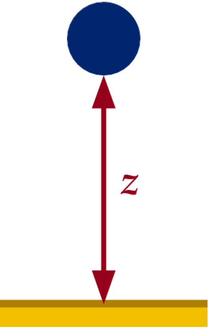
In (1(a)), we display a simple, 1D system with contact: a point mass which makes inelastic impact with the ground at height . The system has state which has freefall motion
| (22) | ||||
| (23) |
For a ground height , the next state either obeys freefall motion, or impacts the ground and comes to rest:
| (24) |
In (1(b)), we fix the ground height to and the initial position to and plot in yellow for . Note the velocity discontinuity due to impact near .
A.1.2 Dynamics Learning
To illustrate the difficulty of fitting a DNN to discontinuity, we consider a simple, unstructured end-to-end dynamics learning setting for the system (24) where we fix and learn the mapping . Specifically, we generate training state transitions , by uniformly sampling points from the graph of in (1(b)), and perturbing each element of and with Gaussian white noise with variance . The data is shown in (1(b)) as yellow dots.
We train a fully connected DNN to predict . The DNN has hidden layers of width and activations, and is trained using Adam with PyTorch default parameters using loss
| (25) |
Training is terminated when the loss converges on a separate, identically distributed validation set. The fully trained network’s output is plotted in blue in (1(b)). The trained DNN is unable to capture the velocity discontinuity well, and predicts significant ground penetration. While stopping early on validation loss prevents the model from overfitting to the noisy training data, the result of this regularization merely produces a smooth regressor, and does not recover important qualitative features of the true system. By a similar notion, any naive regularization that encourages smoothness (e.g. weight decay) will generate similar learned models. Furthermore, an unregularized training process is likely to produce an interpolator of the data, which would exacerbate ground penetration and generate erratic behavior near the discontinuity.
Next, we consider a simple application of ContactNets to the 1D system. Without tangential motion along the surface, there are no frictional behaviors in the system; we therefore forego learning related quantities. We consider the simple case of learning an approximation of the ground height . As in Section 4, we construct the inter-body signed distance, , and contact impulse estimate . Finally, as there are no frictional behaviors in the system, we construct a simplified version of our mechanics-inspired loss (16):
| (26) |
The average of this loss over the data is plotted in (1(c)) in red for different . We learn by minimizing (26) using Adam with identical training hyperparameters and termination conditions as the DNN model. After recovering a good estimate for ground height, we can predict the next state as , shown in red in (1(b)). As we embed the key behaviors of contact directly into our model, we both quantitatively and qualitatively outperform the unstructured baseline model. Despite significant noise in the training and validation data, our method produces a ground height which closely approximates the true in the underlying system.
Given that we predict state transitions using , it might seem natural employ loss , shown in blue in (1(c)), during training. However, because is discontinuous in , the loss is not differentiable or even continuous, leading to numerical challenges. By contrast, our loss is smooth, allowing higher-order methods like Adam to perform well.
A.2 Learning setup

The optimal network structure for End-to-end was empirically determined by varying network width and depth, resulting in hidden layers with neurons and activations. Network inputs are normalized to have zero mean and unit variance. Training is executed using the PyTorch AdamW optimizer with a learning rate of and weight decay of .
The ContactNets models are parameterized as depicted in Figure 7. Object-frame geometry and surface orientation vectors are initialized randomly to their ground-truth values with significant added noise (standard deviation of of their original values). For ContactNets Deep, a separate network is summed in parallel, featuring two hidden layers of neurons with activation. Following the addition of regularizers as described in Appendix A.3 with coefficients , AdamW was used for optimization with a learning rate of and weight decay.
For the ContactNets methods, we require an additional procedure for computing from the parameterization of and a given configuration. This is accomplished by first forwards propagating an input through the network, keeping note of its value before each operation (activation, weight multiplication, etc.), and then backpropagating a Jacobian matrix using the chain rule. Coupling and is critical to ensuring that our learned model produces physically reasonable behavior. We similarly parameterize as the Jacobian of a learned function .
For all models the train-validation-test split is 50-30-20. Each model is trained until its loss fails to improve on the validation set for atleast epochs (smaller datasets were permitted additional epochs) and is subsequently evaluated on the test dataset in Figure 5.
A.3 Learning regularizers
The LCP-based, semi-implicit method of Stewart and Trinkle 1996 is used to simulate rollouts with the learned . To prevent unrealistic simulation artifacts, the following regularizers were added to the loss (16):
A.3.1 Normal–tangent perpendicularity
For each contact, we expect that contact-frame forces applied to the body due to normal and frictional contact forces to be orthogonal by definition; hence, we encourage the corresponding elements of the normal and tangential contact Jacobians and to be perpendicular by penalizing their normalized dot products:
Here, and denote the columns of and that relate to the center of mass position.
A.3.2 Position Jacobian unit norm
Regardless of object or table geometry, geometric analysis would imply that has unit norm. We therefore additionally penalize