Using Under-trained Deep Ensembles to Learn Under Extreme Label Noise
Abstract
Improper or erroneous labelling can pose a hindrance to reliable generalization for supervised learning. This can have negative consequences, especially for critical fields such as healthcare. We propose an effective new approach for learning under extreme label noise, based on under-trained deep ensembles. Each ensemble member is trained with a subset of the training data, to acquire a general overview of the decision boundary separation, without focusing on potentially erroneous details. The accumulated knowledge of the ensemble is combined to form new labels, that determine a better class separation than the original labels. A new model is trained with these labels to generalize reliably despite the label noise. We focus on a healthcare setting and extensively evaluate our approach on the task of sleep apnea detection. For comparison with related work, we additionally evaluate on the task of digit recognition. In our experiments, we observed performance improvement in accuracy from 6.7% up-to 49.3% for the task of digit classification and in kappa from 0.02 up-to 0.55 for the task of sleep apnea detection.
Introduction
Recent advances in Machine Learning (ML) and sensor technology have enabled the possibility of reliable personalized healthcare diagnosis at home. For supervised learning, proper labelling is needed for a classifier to generalize reliably. However, labels can contain errors due to human error, incomplete information, etc. This poses a significant hindrance to proper generalization, which can be very problematic in critical fields like healthcare since it can lead to inappropriate decision making with potentially life-threatening consequences. Furthermore, such errors are typically difficult and labor intensive to fix, since labelling in healthcare requires in most cases expert knowledge.
To address these issues we develop a new approach called Evaluation Probabilities-based Distillation (EPD) based on recent key insights for memorization and predictive uncertainty in Deep Learning (DL) models [1, 2]. EPD utilizes a DL-based ensemble to create new labels and perform Knowledge Distillation (KD) on a new DL model. A key characteristic of EPD is that it under-trains the members of the ensemble, i.e., for each member training stops prematurely, before the loss is properly minimized. As such, EPD utilizes an aggressive form of early stopping to achieve proper generalization, despite the label noise. The main intuition for this choice is straightforward: If a teacher (i.e., the labelling) is partially erroneous but on a high-level correct, under-training can help to avoid learning erroneous details of the teachers beliefs. Furthermore, training multiple models and using different subsets of the data, is used to make the new labelling more robust and reduce variance.
In contrast to the majority of related literature which focuses on computer vision tasks, we focus on sensor time-series data. Specifically, we evaluate EPD for the task of sleep apnea detection. Sleep apnea is a very common yet severely undiagnosed sleep related breathing disorder which affects a large portion of the population. Sleep Apnea events are defined as the cessation of airflow for at least 10 seconds or reduced airflow by at least 30% [3]. To provide a basis for comparison with other works we additionally evaluate on common digit classification tasks (i.e., MNIST and SVHN datasets). For both domains, we explore commonly used artificial label corruption configurations and more realistic settings to measure the success and practical applicability of EPD. The contributions presented in this paper can be summarized as follows: (1) We present a novel DL based method for learning under extreme noise conditions, (2) We showcase state-of-the-art performance across multiple tasks and datasets, and (3) Through a variety of experiments we evaluate the practical feasibility of the proposed approach, and empirically show that it constitutes a viable strategy for all investigated cases 11 1 We include relevant proof-of-concept code at: https://github.com/konkoniknik/Noisy-Labels-EPD .
Method
In this section we discuss previous ideas that inspired EPD, highlight its novel aspects and describe in detail the proposed method. Finally, we discuss the derivation process, and the design choices of EPD.
Inspirations and Characteristics
EPD is inspired by three previous contributions. First, the insight that DNNs learn real patterns first and then noise [2]. This is a consistent characteristic that potentially happens due to the more complex decision boundaries that stochastic label noise tends to create. We exploit this characteristic, by under-training the members of the ensemble, to filter out corrupt labels, through weak representation in the evaluation probabilities (EP, see next section). An obvious issue with this approach is that potential exceptions, that otherwise would have been learned by fine tuning can be easily missed by the under-trained classifiers. This leads us to the second basic inspiration, i.e, to use of ensembles of classifiers as filters to clean noisy datasets from corrupted labels [4]. We use a large committee of under-trained deep neural networks, called base models, trained on different subsets of the training data, and form the EP as out-of-bag predictions of these models. We do this to give classifiers the opportunity to train with subsets that focus on different characteristics of the data. The goal is to enable different base models learn specialized patterns. If this happens successfully, then we expect that the correct class that corresponds to these patterns would be represented in the EP. In contrast to Brodley et al., we utilize random subsampling instead of cross-validation as we (1) want to have many different data combinations for the different models to train with, and (2) need many iterations per datapoint to form consistent EP. Additionally, we label with the EP all classes of each datapoint, instead of tagging a datapoint as correct or incorrect and then removing the incorrect datapoints. This gives us more information for the decisions of the ensemble. Third, we adopt the idea from [5], to focus on states of the model in order to overcome label inconsistencies. However, instead of using the current state of the model (i.e., including an entropy term in our loss), we utilize many under-trained previous states of our model.
Based on the above, with EPD, we draw from the insights of these works in a novel manner and form a new labelling and a new weighing schema to enable a new classifier reliably train despite extreme label noise.
Method Description
We train multiple classifiers . Each classifier is trained (under-trained) on a random subset of a dataset where are datapoints and labels. is of size , and all of size with . We label the remaining data of , i.e., , with . This process is similar to an out-of-bag estimate, but we perform subsampling instead of bootstrap to train . We repeat with all classifiers.
For each datapoint and for each class, we divide the number of classifiers that chose the class by the number of classifiers that labeled . Due to the random sub-sampling process, each datapoint is labelled by a subset of the classifiers in the ensemble. Thus, we end-up with EP for from the subset of the ensemble that labeled . By definition summing up all these class probabilities equals to 1. Algorithm 1 summarizes the creation of the EP.

Then we utilize the EP. We train a new classifier with the EP - or with a convex combination between the EP and the true labels-, as soft labels via knowledge distillation [6]. Additionally, for the training of , we define the weight of based on the maximum evaluation probability of to rescale the samples based on the certainty of the ensemble (Figure 1).
Methodological Derivation: Training with
EPD is designed to refine the ensemble filter from [4]. Assuming a dataset , the empirical risk has normally the following form:
| (1) |
with , and , is a surrogate of the 0-1 loss and the parameter vector of a classifier . However, after a filter like the ensemble from [4] has been applied, the empirical risk is re-weighted with the following weighting scheme: The datapoints that fail the filter gain a priority of 0 and the ones that pass the filter gain equal priority. Formally, we define the filter as a function where is the input space, 0 corresponds to failure and 1 to success. Thus, we can partition into two subsets, i.e., comprising datapoints that have failed () and those that have succeded () as such: and . Now the empirical risk takes the following form:
| (2) |
with and . Because we utilize an ensemble of deep models that perform conditional density estimation, an approximation of the conditional distribution for the training data is formed through the EP. Thus, we want to utilize the proposed method not only as filter but also to correct labels for which the ensemble exhibits a high probability that they are wrong. This probability is reflected in the EP. As such, we can generalize to identify whether a certain condition is satisfied. Then for the data that satisfy this condition, we can correct the label. We define:
| (3) |
where corresponds to the EP vector for datapoint , and corresponds the element of for class . is a simple filter which filters data based on the confidence of the EP. We base our final empirical risk design on this filter. If is 0, then is filtered-out. If is 1 then is not filtered-out. If is 2 then is not filtered-out and we change the class of to . In Eq. 3, we use since is defined only discretely for the datapoints of . In this case, we use as condition to change the label a threshold () for the maximum . This means that for , we change to , if the maximum exceeds . Similarily, if the maximum does not exceed , we do not include the sample in the training data of . We define three non-intersecting sets , and , with . Now, the empirical risk becomes:
| (4) |
with , and . With this extension we can allow corrections of labels as a pre-training step if certain conditions are being met. However, we identify two issues with this design: (1) it could be difficult to properly tune parameters and , and (2) it does not map directly the confidence of the ensemble for a class of a datapoint onto the labelling and the weights of the weighting schema. Based on these requirements the following two modifications can be made: First, the maximum probability of the of can be used as a weight of in the weighting schema of the empirical risk. Second, a convex combination of the true label and the EP can be used instead of training directly with the true labels. In our case, the maximum probability can again be used as the convex combination coefficient. With these two modifications, the threshold parameters are removed, and the confidence of the ensemble is directly captured. Furthermore, the characteristics of are preserved but with more focus on the EP than the real labels, which is desirable in an extreme noise setting. The final empirical risk takes the form:
| (5) |
with , and . Thus, the original label will be mostly used and the sample will be de-prioritized during training, if the ensemble is not confident for a sample. If the ensemble is highly confident for a sample, the opposite will happen and regardless of label, the EP will dominate. Since the EP become more prominent and based on our empirical investigation, we simplify this form and use directly EP as labels (i.e., in Eq. 5, ). With this last change the use of the chosen weighting schema becomes less essential for the de-prioritization of erroneous labels. Instead, it acts as a scaling factor during training for the samples which the ensemble is more confident of (i.e., less entropy).
Data and Experiment Description
To evaluate EPD, we use the following principle throughout our experiments: we mainly use datasets with very high generalization performance which we call clean datasets. Then we corrupt the clean training datasets, evaluate on the clean test sets, and expect labels in the test set as the ground truth. This section describes the datasets and experiments using randomized label corruption as it is common in related literature, and experiments using "realistic" corruption to better reflect noisy labels in real world applications.
Data
In contrast to the main body of related literature, we focus on medical time series data. We use data from Polysomnography (PSG) in sleep laboratory for OSA diagnosis. This data comprises a wide range of physiological signals, including the electrocardiogram (ECG), electroencephalogram (EEG), oxygen saturation (Sp02), heart rate, blood pressure and respiration from the abdomen (RespA), chest (RespC) and nose (NAF) etc. Since we want to capture a realistic application of EPD for a common medical condition, and explore its applicability in various domains, we focus on respiratory sensor data. We mainly use the Apnea-ECG [7, 8], () which is an open PSG dataset from Physionet, containing RespA, RespC, NAF, SpO2 and ECG sensor data. has been used in the Computers in Cardiology challenge and contains high quality data. In 8 recordings contain data from all sensors. Each recording has a duration of 7-10 hours. Labels are given for every one-minute window of breathing, and identify which minutes are apneic and which are not. We aim to capture the behavior of EPD for data gathered from all different sensor devices that focus on respiratory signals. Thus, we evaluate on signals gathered with the use of a respiratory belt on the abdomen of the patient (RespA:), with the use of a nasal thermistor from the nose (NAF:), and with the use of a pulse oxymeter that measures oxygen saturation in the blood (Sp02:). We choose RespA over RespC as the belt sensor due to its better behavior in our preliminary evaluation. Furthermore, the lower quality MIT-BIH [9], () dataset is used to corrupt . Finally, we use two well-established datasets from digit classification, i.e., MNIST [10], () and SVHN [11],() to provide a basis for comparison with related literature and to investigate the generalizability of EPD on different tasks. We discuss the datasets in more detail the Technical Appendix.
Experiment Description
The goal of the experiments is to quantify the impact that EPD has on classification performance. Since a noisy baseline makes evaluation non-trivial due to the lack of reliable ground-truth, it is common practice to use a noise-free dataset and add randomized noise to corrupt the training labels. While this can guarantee correct evaluation results, it is a strategy which in many cases is unrealistic. Therefore, we perform two types of experiments.

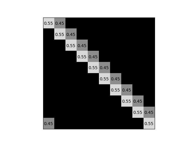
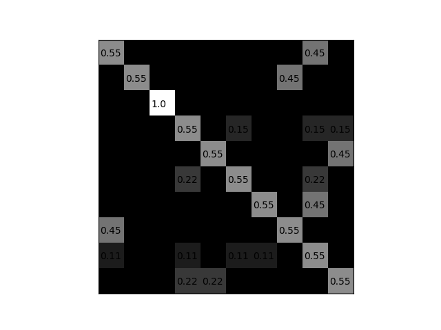
For the first experiment type, we use the clean datasets (i.e., , and ) and corrupt them using artificial randomized noise sources. Then we train with the corrupted training data, and evaluate on the clean test data, to get an indication of how well EPD can generalize despite the noise. To corrupt the datasets we use of a noise transition matrix to change the class of a sample to another class with the probability mapped in the respective element of the matrix. We experiment with the two types of transition matrices commonly used in literature, i.e., pair and symmetry (shown in Figures 2(a) and 2(b)). For the second experiment type, we perform different experiments where we corrupt the datasets in more realistic and task-specific ways than in the previous case. For the digit classification task, we create a noise transition matrix based on common human Alphanumeric misidentification patterns indicated by relevant medical literature [12]. We show the noise transition matrix for this task in Figure 2(c). Then, for the apnea dataset we: (1) introduce realistic label noise and a domain shift by adding data into the training data and (2) investigate whether the proposed approach can be used to enhance the labelling of apnea data of a non-expert.
Evaluation
In this section we describe the preprocessing steps we performed, the decisions we made regarding general and method-specific hyper-parameter values, and the experiments to evaluate the proposed approach. As baseline, we use in all experiments the results gained with the model, trained with equal weights per datapoint and with the true labels (i.e., no KD) regardless of noise level.
Preprocessing, Metrics and Hyper-Parameters
In all experiments, we execute the same preprocessing steps for the datasets. We rescale the pixel values of all samples of the digit datasets and from 0-255 to 0-1. Additionally, for we restructure the data in similar form to (from to ). Furthermore, both digit datasets have a predefined test sets which we will use.
In both sleep apnea datasets the data is standardized per physiological signal, downsampled to 1Hz, shuffled randomly and divided into train and test sets. We perform the last step since no predefined test sets exist in the respiratory datasets. The percentage of data used as test set changes depending on the experiment. Furthermore, the labels in are given every 30 seconds and in every 60 seconds. Therefore, we adapt the labelling in to 60 seconds with the following rule: if both 30 second labels are non-apneic then the 60 seconds label is non-apneic, elsewise it is apneic.
We evaluate the classification performance on the clean test set. For the Digit Classification experiments we use Accuracy as performance metric. For Apnea Detection, which is a two class problem, we use the Kappa statistic [13], since Kappa takes into account random agreement. This makes it a suitable choice for the task of apnea detection. Additionally, for all results the standard error of the mean is presented.
In all experiments we use convolutional neural networks with a batch size of 128, and a learning rate of 0.001. For brevity, we include the architectures used in the Technical Appendix. For the evaluation we follow the conventions from [14], i.e., in all experiments the baseline model and are trained for 200 epochs, and the generalization performance is calculated from the average performance of the last 10 epochs.
Furthermore, base models are used for EPD, 1/3 of the training dataset is used as evaluation dataset, and 2/3 for the actual training. In most experiments, the base models are trained for 4 epochs. The choice of the amount of epochs to train the base models is not trivial since the use of a noisy validation set to choose the best performing epoch does not guarantee good generalization performance on the clean test set. Empirical investigation showed that a more reliable metric is the minimum mean entropy of the EP. Furthermore, this metric is in-line with the under-training principle. The minimum EP entropy is reached in most configurations early during training, and close to the epoch where the maximum generalization performance is reached on the clean test set. We discuss in more detail the reasoning followed to choose the values of these hyper-parameters in the Technical Appendix.
Randomized Corruption
We use the Pair and Symmetry noise transition configurations and investigate the performance of EPD in comparison to the baseline, for various noise levels.
Digit Classification
Table 1 shows the results for the and datasets under the Pair and Symmetry label corruption configurations. As expected EPD outperforms Baseline training in all cases by a wide margin. Notice that the pair noise configuration is harder than the symmetry since each class can only change to the one other class. As a result this class will be overly represented in place of the original class, making the training inherently harder, especially as the corruption probability approaches 50%.
| Method | Pair-0.40 | Pair-0.45 | Sym.-0.20 | Sym.-0.50 | Sym.-0.63 |
|---|---|---|---|---|---|
| S:Baseline | 0.5870.001 | 0.5230.002 | 0.8350.001 | 0.5930.002 | 0.4290.002 |
| S:EPD | 0.8490.002 | 0.7360.005 | 0.9050.001 | 0.8770.001 | 0.850.001 |
| M:Baseline | 0.6210.002 | 0.5610.002 | 0.9140.001 | 0.6390.002 | 0.4730.001 |
| M:EPD | 0.9790.001 | 0.950.002 | 0.9810.001 | 0.9730.001 | 0.9660.001 |
Figure 3 shows several performance characteristics for the two datasets. In Figure 3,(a),(b) we notice for , for the different corruption configurations and noise levels that with decreasing true class representation, the performance of the baseline decreases steadily. In contrast, EPD manages to perform well even in cases of extreme noise, (e.g., the cases of Symmetry-0.76 or Pair-0.48). In the second row, (Figure 3, (d)) we show the model’s performance throughout training for the baseline in comparison to EPD for . The initial performance of Baseline is high, but it quickly drops, as expected. Contrary to that, , which is trained with EPD is mostly not affected from the label noise. We include additional similar graphs for other noise configurations in the Technical Appendix.


Though EPD is inherently a simple method, we achieve state-of-the-art results compared to other well-established methods like [14] () or [15] (S). We expect that the success of EPD depends on: (a) the ability of the base classifiers to prioritize learning clean samples during learning, i.e., under-training is successful, (b) on the ability of the ensemble to compensate from erroneous beliefs on certain datapoints.
Sleep Apnea Detection
For the sleep apnea detection experiments, we investigate the proposed approach with three signals from the dataset (i.e., Resp A, NAF and Sp02). Similarly as before we corrupt the labels with random noise based on the noise transition matrix. However, in this case, we only have two classes, i.e., apneic and non-apneic minutes. Thus, we practically investigate the Pair noise type.
Table 2 shows the comparative results between Baseline training and EPD across the three respiratory sensors. In all cases, we notice a steep drop in performance for the Baseline with increasing noise. The performance drop is substantially smaller for EPD. Note that the widest margins in performance difference between Baseline and EPD is for the NAF signal. Figure 3 (c) shows the performance (kappa) for the NAF signal, throughout training for noise level of 45 percent (Pair-45, average of 3 runs). We observe similar characteristics as before. The Baseline has a steep drop early-on in the training process. This is not the case for EPD, which is only initially affected by the noise level, and not throughout the whole training process.
Significance for Condition Detection: From the results we notice that the performance for all signals is significantly affected from the noisy labelling, especially for larger noise levels.This means that a "careless" annotator would affect negatively the correct identification for this medical condition. However, the use of the proposed method is highly likely to allow an expert have a much wider error margin during labelling. Depending on the goal, this margin can be translated as the relaxation of the constraints placed upon the quality of the annotator’s expertise.
| Noise | Pair-0.20 | Pair-0.35 | Pair-0.45 |
|---|---|---|---|
| NAF:Baseline | 0.5810.004 | 0.2940.005 | 0.1030.008 |
| NAF:EPD | 0.8880.003 | 0.8290.005 | 0.5840.020 |
| RespA:Baseline | 0.5680.007 | 0.2670.007 | 0.0980.010 |
| RespA:EPD | 0.8510.003 | 0.8130.007 | 0.5470.020 |
| Sp02:Baseline | 0.6600.007 | 0.4250.006 | 0.1790.013 |
| Sp02:EPD | 0.8280.004 | 0.8110.003 | 0.6440.025 |
Realistic Corruption
In this section we evaluate EPD on realistic sources of noise.
Digit Classification: Alphanumeric Misidentification Patterns
In medical literature [12], common alphanumeric misidentification patterns are identified. We use these patterns to create a noise transition matrix (Figure 2 (c)) to corrupt the true labels in a realistic manner. We use noise level of 0.45, since it is a representative level of an extremely noisy setting. Furthermore, for some classes we are not able to exceed noise level of 0.5 without the noise overtaking the true class. We assign this probability mass equally to the classes that can potentially be swapped in place of the true class. For example, in the case of digit 3, which label can be changed to 5,8 or 9, we assign equal probability of 0.15 to these three swaps. We call this type of corruption Alphanumeric-0.45. We execute the experiment for and datasets. We repeat the experiments 10 times.
For the average accuracy of Baseline is: 0.6330.002, and with EPD: 0.9490.001. For : Baseline: 0.6120.001, EPD: 0.7760.002. As expected, EPD significantly outperforms Baseline in both datasets.
Apnea Detection: Corrupting Clean Dataset with Noisy Dataset
We combine part of and to create a joint training dataset. is noisier than in terms of data and labelling. Thus, we corrupt the clean training datapoints of with the noisier datapoints. We use a test set comprised only with datapoints from (we use 75% of ). We use the NAF signal as it is the most common signal of . We investigate different percentages of inclusion of the remaining 25% of in the new joint training dataset (i.e., we include 100% of and either 25%,12.5%,5%,1.25%,or 0% of ). Less inclusion of data in the Joint training dataset corresponds to "noisier" labels in the training data. We repeat the experiment 20 times.


In all cases, EPD is superior to Baseline training, as expected (Figure 4 (a)). As smaller percentages of are included in the Joint training data, we expect drop in performance due to the noisy labelling and the domain shift imposed in the input space. Thus, we expect both cases to drop in performance as we include smaller parts of . Indeed, we observe such a behavior from Figure 4 (a). Notice also that the difference between Baseline and EPD increases as the percentage of decreases. In Figure 4 (b), we show the test performance during training, for inclusion of 0%. We notice a similar behavior as in the previous sections.
Apnea Detection: Non-Expert Labelling
A non-expert labelled a small subset of (corresponding to 5% of the whole data), for the three sensors we utilize in this work i.e.,Resp A, NAF, and Sp02. To do this, a "hint" of 10 randomly sampled datapoints was presented to the non-expert together with their true labels, to help the non-expert learn patterns per-class. Then, the non-expert proceeded to the actual labelling of a random part of (5% of ). We utilize this dataset and train a model with these data and labels. We evaluate the generalization performance of the model with the other 95% of dataset. We repeat this procedure for all three sensors. In this experiment, the majority of conventions and configurations are as the ones described above. However, since we have a very small training dataset, we need to keep per base classifier as much of the data as possible for training. For this reason we use 1/10 of the training data as evaluation datasets instead of 1/3. Furthermore, to partially compensate for this and create reliable EP, we use more base models () than in the default configuration. Finally, based on the EP-entropy criterion (see Technical Appendix) used to determine how much to train the base classifiers, we notice that 4 epochs are insufficient for such a small dataset. Thus, we train for 20 epochs the base models. Again, we compare the baseline to EPD. Given the non-expert labels, we repeat the experiment (i.e., training and evaluating on the noise-free test set) 10 times.
The agreement of the non-expert labelling with the true labels (i.e., the expert’s labelling) for the three sensors is (Accuracy): Resp A: 0.855, NAF: 0.94, Sp02: 0.745. The generalization performance on the test set (Kappa) is: Resp A: Baseline: 0.730 0.003, EPD: 0.7880.001; NAF: Baseline: 0.8380.004, EPD: 0.8600.004; Sp02: Baseline: 0.5880.008, EPD: 0.7430.005. In all cases EPD outperforms the baseline. The results are statistically significant based on the one-tailed t-test for all sensors. A clear correlation between the performance difference of Baseline and EPD on the one hand, and the agreement between labellings on the other hand can be observed.
Discussion
From the above experiments, we identify that EPD offers a reliable approach for training under conditions of extreme label noise, even in realistic settings as long as proper parametrization conditions are being met. The results of our experiments are promising, and showcase the versatility of EPD even when the strict definition of noise is laxed.
An important empirical observation is that, as expected, EPD cannot provide a reliable training regime in cases where the noise levels are so high that they form a bias towards a wrong class, i.e., where, for certain regions of the feature space a consistent wrong class belief is formed by an erroneous labelling strategy. In such cases, where the majority of labels leans on one wrong class in such a way that it can be wrongfully learned, the under-training could potentially have a negative effect in the learning of the correct decision boundaries. However, these cases correspond to principle mistakes of the labelling strategy, and not in occasional mistakes that constitute noise in the labels. Examples of such cases in the medical domain could be that of an untrained annotator which has misunderstood basic identifiers of a condition, and makes repeatedly the same errors, or a rule-based software that is not properly tuned for a particular individual. We hypothesize that for such cases a noise correction learning framework would not be the better choice, and different bias correction strategies would need to be implemented to help a new model to generalize correctly. However, for the problem EPD is designed to tackle it yields promising and reliable empirical results in a variety of tasks and domains.
Related work
There exist a large body of literature addressing corrupt labels, which is well captured in [16]. From this body of work, we present only works that have key similarities to our own. We separate this section based on two types of works: (1) works that use multi-network frameworks or KD (2) works that use data weighing strategies.
Many works utilize KD or multi-network configurations to achieve better training under label noise. Examples include [5, 17], which utilize the current state of the model and update the prediction labels with the current model prediction . Other approaches that utilize a student teacher configuration include [18, 19]. [19], propose the use of KD from an auxiliary model trained on a small clean dataset to guide the training of a model trained on a larger noisy dataset using a convex combination of the noisy labels and the output of the auxiliary model. We experimented with a convex combination of the true label and EP. However, our experiments show that the results with the convex combination were inferior to those with only EP. [20] train two networks which are only updated when they disagree for a given instance. [1] propose the use of ensembles of DNNs to quantify predictive uncertainty. The insights obtained from this work are used together with MC-dropout [21] by [22] to detect noisy labels. They propose the use of uncertainty estimates to identify a good epoch for relabelling a percentage of the lowest confidence data. Contrary to this work, we base our decision of how much to train on the entropy of the EP. Furthermore, another key difference between EPD and the above approach is that in EPD the EP are formed as out-of-bag estimates from the different base classifiers of the ensemble. As such, they represent a form of pseudo-generalization. None of the base classifiers contributing to the EP for a datapoint has made any association about its label beforehand. Finally, [23] create out-of-fold logits based on the predictions of base classifiers with the use of a base-ensemble of heterogeneous classifiers and LBGM [24]. Despite the similarities with this approach, we utilize under-training as a way to more efficiently identify noisy labels and exploit the out-of-fold predictions (EP) as a form of curriculum for the training process. Furthermore, we use the EP to identify the proper amount of training for the ensemble’s base models.
Regarding data re-weighing strategies, [25] observe that training accuracy is evolving differently for noisy and clean samples. Based on this observation they propose alternating between selecting a subset of the training samples that has the smallest loss, and training with this sample. Other similar approaches include [26, 27, 28].[28] identify incorrect labels with the use of a DNN. Labels that differ from the predictions of the DNN (trained on the noisy dataset) are removed. The remaining data are sorted based on prediction confidence and labels below a certain confidence threshold are also removed. Then semi-supervised learning is applied to train with both data that contain and do not contain labels. A different approach partially based on data reweighing is co-teaching [14]. Han et al. utilize two networks, and each network learns with the subset of the extracted mini-batch, which contains the instances with the smallest loss of the other network. [29] expand upon co-teaching by applying the same procedure, but focusing on a subset of the data, which contains only points for which the two networks disagree. [30] introduce MentorNet, which learns a curriculum to weigh training samples’ priority during the training of a student network. A key difference between the above approaches and EPD stems from the fact that the weighting schema in EPD originates from the accumulative knowledge of a deep ensemble. However, in EPD the reweighing plays a secondary role due to the use of KD, and it is only used to de-prioritize uncertain samples.
Conclusions and Future Work
In this work we investigated a simple, yet effective approach for successful learning under extreme label noise. Contrary to related literature, EPD re-uses the cumulative knowledge of the ensemble back in the training data in such a way that it takes advantage of the generalization capabilities of independent parts of the ensemble and forms new labels for the training data. With the use of KD, a new model is trained with the new labels. As such, the ensemble is used only for the synthesis of the new labels, and only the new model needs to be used after the procedure is finished.
We empirically show the success of EPD in a variety of settings, configurations and noise levels, for two real world tasks. We observe that EPD can offer a general and reliable solution to the problem of learning under label noise. Our results serve as indicators of the applicability of EPD towards more reliable condition diagnosis. Labelling assistance can be another interesting application direction.
A natural next step is the identification of more consistent errors in regions of the feature space which are based on wrong beliefs of the annotator and not random mistakes. We hypothesize that an approach which incorporates elements from unsupervised learning could potentially be able to assist towards the identification of these wrongful biases. Based on this, we want to incorporate such elements to the EPD framework and provide a more general solution.
References
- [1] Balaji Lakshminarayanan, Alexander Pritzel, and Charles Blundell. Simple and scalable predictive uncertainty estimation using deep ensembles. In Advances in neural information processing systems, pages 6402–6413, 2017.
- [2] Devansh Arpit, Stanisław Jastrzębski, Nicolas Ballas, David Krueger, Emmanuel Bengio, Maxinder S Kanwal, Tegan Maharaj, Asja Fischer, Aaron Courville, Yoshua Bengio, et al. A closer look at memorization in deep networks. In Proceedings of the 34th International Conference on Machine Learning-Volume 70, pages 233–242. JMLR. org, 2017.
- [3] AASM. Aasm sleep apnea. https://www.medscape.com/answers/295807-53441/what-is-the-aasm-definition-of-apnea, 2020. [Online; accessed 10-10-2019].
- [4] Carla E Brodley and Mark A Friedl. Identifying mislabeled training data. Journal of artificial intelligence research, 11:131–167, 1999.
- [5] Scott Reed, Honglak Lee, Dragomir Anguelov, Christian Szegedy, Dumitru Erhan, and Andrew Rabinovich. Training deep neural networks on noisy labels with bootstrapping. arXiv preprint arXiv:1412.6596, 2014.
- [6] Geoffrey Hinton, Oriol Vinyals, and Jeff Dean. Distilling the knowledge in a neural network. arXiv preprint arXiv:1503.02531, 2015.
- [7] Ary L Goldberger, Luis AN Amaral, Leon Glass, Jeffrey M Hausdorff, Plamen Ch Ivanov, Roger G Mark, Joseph E Mietus, George B Moody, Chung-Kang Peng, and H Eugene Stanley. Physiobank, physiotoolkit, and physionet: components of a new research resource for complex physiologic signals. circulation, 101(23):e215–e220, 2000.
- [8] Thomas Penzel, George B Moody, Roger G Mark, Ary L Goldberger, and J Hermann Peter. The apnea-ecg database. In Computers in Cardiology 2000. Vol. 27 (Cat. 00CH37163), pages 255–258. IEEE, 2000.
- [9] Yuhei Ichimaru and GB Moody. Development of the polysomnographic database on cd-rom. Psychiatry and clinical neurosciences, 53(2):175–177, 1999.
- [10] Yann LeCun, Léon Bottou, Yoshua Bengio, and Patrick Haffner. Gradient-based learning applied to document recognition. Proceedings of the IEEE, 86(11):2278–2324, 1998.
- [11] Yuval Netzer, Tao Wang, Adam Coates, Alessandro Bissacco, Bo Wu, and Andrew Y Ng. Reading digits in natural images with unsupervised feature learning. 2011.
- [12] Matthew Grissinger. Misidentification of alphanumeric symbols plays a role in errors. https://www.ncbi.nlm.nih.gov/pmc/articles/PMC5614409/, 2017. [Online; accessed 2-June-2020].
- [13] Jacob Cohen. A coefficient of agreement for nominal scales. Educational and psychological measurement, 20(1):37–46, 1960.
- [14] Bo Han, Quanming Yao, Xingrui Yu, Gang Niu, Miao Xu, Weihua Hu, Ivor Tsang, and Masashi Sugiyama. Co-teaching: Robust training of deep neural networks with extremely noisy labels. In Advances in neural information processing systems, pages 8527–8537, 2018.
- [15] Kimin Lee, Sukmin Yun, Kibok Lee, Honglak Lee, Bo Li, and Jinwoo Shin. Robust inference via generative classifiers for handling noisy labels. arXiv preprint arXiv:1901.11300, 2019.
- [16] Davood Karimi, Haoran Dou, Simon K Warfield, and Ali Gholipour. Deep learning with noisy labels: exploring techniques and remedies in medical image analysis. arXiv preprint arXiv:1912.02911, 2019.
- [17] Yaoyao Zhong, Weihong Deng, Mei Wang, Jiani Hu, Jianteng Peng, Xunqiang Tao, and Yaohai Huang. Unequal-training for deep face recognition with long-tailed noisy data. In Proceedings of the IEEE Conference on Computer Vision and Pattern Recognition, pages 7812–7821, 2019.
- [18] Lequan Yu, Shujun Wang, Xiaomeng Li, Chi-Wing Fu, and Pheng-Ann Heng. Uncertainty-aware self-ensembling model for semi-supervised 3d left atrium segmentation. In International Conference on Medical Image Computing and Computer-Assisted Intervention, pages 605–613. Springer, 2019.
- [19] Yuncheng Li, Jianchao Yang, Yale Song, Liangliang Cao, Jiebo Luo, and Li-Jia Li. Learning from noisy labels with distillation. In Proceedings of the IEEE International Conference on Computer Vision, pages 1910–1918, 2017.
- [20] Eran Malach and Shai Shalev-Shwartz. Decoupling" when to update" from" how to update". In Advances in Neural Information Processing Systems, pages 960–970, 2017.
- [21] Yarin Gal. Uncertainty in deep learning. University of Cambridge, 1:3, 2016.
- [22] Jan M Köhler, Maximilian Autenrieth, and William H Beluch. Uncertainty based detection and relabeling of noisy image labels. In Proceedings of the IEEE Conference on Computer Vision and Pattern Recognition Workshops, pages 33–37, 2019.
- [23] Pavel Ostyakov, Elizaveta Logacheva, Roman Suvorov, Vladimir Aliev, Gleb Sterkin, Oleg Khomenko, and Sergey I Nikolenko. Label denoising with large ensembles of heterogeneous neural networks. In Proceedings of the European Conference on Computer Vision (ECCV), pages 0–0, 2018.
- [24] Guolin Ke, Qi Meng, Thomas Finley, Taifeng Wang, Wei Chen, Weidong Ma, Qiwei Ye, and Tie-Yan Liu. Lightgbm: A highly efficient gradient boosting decision tree. In Advances in neural information processing systems, pages 3146–3154, 2017.
- [25] Yanyao Shen and Sujay Sanghavi. Learning with bad training data via iterative trimmed loss minimization. arXiv preprint arXiv:1810.11874, 2018.
- [26] Cheng Xue, Qi Dou, Xueying Shi, Hao Chen, and Pheng-Ann Heng. Robust learning at noisy labeled medical images: applied to skin lesion classification. In 2019 IEEE 16th International Symposium on Biomedical Imaging (ISBI 2019), pages 1280–1283. IEEE, 2019.
- [27] Jun Shu, Qi Xie, Lixuan Yi, Qian Zhao, Sanping Zhou, Zongben Xu, and Deyu Meng. Tug the student to learn right: Progressive gradient correcting by meta-learner on corrupted labels. arXiv preprint arXiv:1902.07379, 2019.
- [28] Yifan Ding, Liqiang Wang, Deliang Fan, and Boqing Gong. A semi-supervised two-stage approach to learning from noisy labels. In 2018 IEEE Winter Conference on Applications of Computer Vision (WACV), pages 1215–1224. IEEE, 2018.
- [29] Xingrui Yu, Bo Han, Jiangchao Yao, Gang Niu, Ivor W Tsang, and Masashi Sugiyama. How does disagreement help generalization against label corruption? arXiv preprint arXiv:1901.04215, 2019.
- [30] Lu Jiang, Zhengyuan Zhou, Thomas Leung, Li-Jia Li, and Li Fei-Fei. Mentornet: Learning data-driven curriculum for very deep neural networks on corrupted labels. arXiv preprint arXiv:1712.05055, 2017.
- [31] Stein Kristiansen, Mari Sønsteby Hugaas, Vera Goebel, Thomas Plagemann, Konstantinos Nikolaidis, and Knut Liestøl. Data mining for patient friendly apnea detection. IEEE Access, 6:74598–74615, 2018.
Ethics Statement
In the context of sleep apnea detection, noisy or inconsistent labelling is a real problem. Even trained sleep experts disagree to a certain extent about apneic and non-apneic events. Inconsistent labelling can lead to wrong conclusions with respect to treatment. Thus, reliable classification for such tasks can have a positive impact on well-being and reduce costs in the health sector. The primary motivator for the approach presented in this work is such a healthcare-oriented setting. However, since the approach is general, it can also be used in other settings.
Appendix A Appendix A: Datasets
In this Appendix we describe in more detail the datasets used in our experiments:
- •
MNIST () [10] is a well-known dataset which contains 60000 2828 images of digits (handwritten black and white images of 0-9) as a training set. The test set is composed of 10000 images.
- •
SVHN ()[11] is a real-world image dataset. is obtained from house numbers in Google Street View images. It contains 73257 digits (32 32 colored images) for training, 26032 digits for testing, and 531131 less difficult samples that can be used as additional training data. We use only the original training dataset of 73257 digits.
- •
Apnea-ECG ()[7, 8] is an open PSG dataset from Physionet, containing RespA, RespC, NAF, SpO2 and ECG sensor data. has been used in the Computers in Cardiology challenge [8] and contains high quality data. From the 35 recordings in the dataset, 8 recordings (namely a01-4,b01,c01-3) contain data from all sensors. Each recording has a duration of 7-10 hours. The sampling frequency of all sensors is 100Hz, and labels are given for every one-minute window of breathing. The labels identify which minutes are apneic and which are not (i.e., if a person experiences an apneic event during this minute). In this work, we aim to capture the behavior of EPD for data gathered from all different sensor devices that focus on respiratory signals. Thus, we evaluate on respiratory signals gathered with the use of a respiratory belt on the abdomen of the patient (RespA:), with the use of a nasal thermistor from the nose (NAF:), and with the use of a pulse oxymeter that measures oxygen saturation in the blood of the patient (Sp02:).
- •
MIT-BIH () [9] is an open dataset containing recordings from 18 patients, with different respiratory sensor signals. In 15 recordings, the respiratory signal has been collected with NAF. Since this is the signal with the most recordings in , we use it for our experiments. Due to misalignment of the different signals and lack of labels for the apneic class in 4 recordings, we utilize 11 of the 15 recordings (slp60,slp41 and slp45 and slp67x are excluded). Related literature [31] suggests that the data/labelling quality of the dataset is low. This leads to low classification performance for compared to . This characteristic of is important for our experiments. The labels are given for every 30 seconds and the sampling frequency of all sensors is 250Hz.
| Architectures | |||
|---|---|---|---|
| MNIST | SVHN | Apnea | |
| Conv,(MP,BN) | |||
| Conv,(MP,BN) | |||
| Conv,(MP,BN) | |||
| FC,D,(BN) | |||
| FC,D,(BN) | |||
| out | |||
Appendix B Appendix B: EPD Hyper-Parameter Tuning
In this Appendix, we discuss the hyper-parameter tuning for EPD.
Epoch Choice for Base Classifiers
One of the most important parameters of EPD is the number of epochs used to train the base classifiers . We base our choice on the insights from [2], and we choose to under-train the networks, so that we avoid fitting on the noisy labels. We notice that the entropy of the EP is a relatively reliable empirical measure of the generalization capabilities of the ensemble, which directly impacts the generalization capabilities of . We hypothesize that the use of different evaluation datasets for the different base classifiers as well as the use of generalization for the specification of the EP have a beneficial effect towards appropriate calibration of the EP of the different samples. Based on this hypothesis we use the mean entropy of the EP as an estimate of the true correctness likelihood of the dataset. Thus, we choose the number of epochs with which we train the base classifiers based on the minimum mean EP entropy reached among a set of different potential values for . Figure (5(d)) presents the performance-to-EP-Entropy comparison for (Orange-Blue respectively). We notice a clear correlation between the two measures. Similar associations were made across the majority of the different noise configurations and datasets.


Number of Base Classifiers
The number of base classifiers is important for the performance of EPD. Empirically, the best results are reached when a minimum number for is satisfied. When surpasses this threshold no further improvement is observed. We include examples for the and datasets in Figures (5(a)), (5(c)) for the Pair-0.45 configuration, and the default parameterization. In both datasets, the performance stabilizes after a certain value of (50 models for and 100 models for ).
Size of Evaluation Dataset
For the creation of the , we need to separate the training dataset multiple times into a subset used for training the base models and a subset used for evaluation, for which predictions are being made. A critical question regards how large each of these subsets will be. Using too small training subset will result in low generalization capability. On the other hand, using too large training subset, for a fixed , would result in low precision in the creation of the . This could negatively impact training of . In Figure (5(c)) we include the generalization performance of trained with EPD on the NAF: dataset across different evaluation- dataset sizes. We show on the x-axis the percentage of the training dataset used for evaluation. In each of the cases, the rest of the training dataset is used for training the base models. The training dataset is reshuffled per-base model. The experiment is performed with the Pair-0.45 configuration.
We notice that the performance increases substatially for smaller sizes of evaluation datasets, i.e., more data for the actual training. However, after a certain point, the performance starts to drop. We see this in Figure (5(c)) for evaluation size of 4% We attribute this phenomenon to the poor formation of the due to the small percentage of evaluation dataset in conjunction with the small for this size. We can circumvent this by increasing at the expense of additional training time.
Appendix C Appendix C: Architectures
In this Appendix (Table 3) we include the architectures of the networks used in our experiments.
Appendix D Appendix D: Additional Results
In this Appendix, we include additional results from our experiments. Specifically, we include the performance across all epochs for the Pair-45 (Fig. (6(a))), Symmetry-37 (Fig. (6(b))), Symmetry-37 (Fig. (6(c)))and Pair-20 (Fig. (6(d))) configurations.


Appendix E Appendix E: Additional Implementation Details
All experiments were performed on nvidia geforce rtx 2080 ti graphics card. Python 3.6.9 and Tensorflow 1.14.0 were used.