Improved gradient descent-based chroma subsampling method for color images in VVC
Abstract
Prior to encoding color images for RGB full-color, Bayer color filter array (CFA), and digital time delay integration (DTDI) CFA images, performing chroma subsampling on their converted chroma images is necessary and important. In this paper, we propose an effective general gradient descent-based chroma subsampling method for the above three kinds of color images, achieving substantial quality and quality-bitrate tradeoff improvement of the reconstructed color images when compared with the related methods. First, a bilinear interpolation based 22 () color block-distortion function is proposed at the server side, and then in real domain, we prove that our general 22 color block-distortion function is a convex function. Furthermore, a general closed form is derived to determine the initially subsampled chroma pair for each 22 chroma block. Finally, an effective iterative method is developed to improve the initially subsampled -pair. Based on the Kodak and IMAX datasets, the comprehensive experimental results demonstrated that on the newly released versatile video coding (VVC) platform VTM-8.0, for the above three kinds of color images, our chroma subsampling method clearly outperforms the existing chroma subsampling methods.
Keywords Bayer color filter array (CFA) image chroma subsampling digital time delay integration (DTDI) CFA image block-distortion model versatile video coding (VVC) quality-bitrate tradeoff RGB full-color image
1 Introduction

In this study, we consider the chroma subsampling problem for the three kinds of color images, namely the RGB full-color image , the Bayer color filter array (CFA) image [1] which will be introduced in Subsection 1.1.2, and the digital time delay integration (DTDI) CFA image [2] which will be introduced in Subsection 1.1.3. For convenience, let the above three kinds of color images be denoted by the set CI = {, , }.
Before encoding the color image CI = {, , }, except , and should be demosaicked to RGB full-color images. To demosaick to a RGB full-color image, several demosaicking methods [3], [4], [5] can be used, and in our study, the demosaicking method proposed by Kiku et al. [4] is used. To demosaick to a RGB full-color image, based on Kiku et al.’s residual interpolation idea, we developed a demosaicking method whose execution code can be accessed from the website [6]. Furthermore, following BT.601 [7], the RGB full-color image is transformed into a YUV image by using the following RGB-to-YUV conversion formula:
| (1) |
in which and indicate the RGB pixel and the converted YUV pixel triple-values, respectively, at the location , , according to the zigzag order in each 22 RGB and YUV block-pair. It is noticeable that all discussion in this paper can be applied to the YCbCr color space because the color conversions, RGB-to-YCbCr and YCbCr-to-RGB, are also linear as the color conversions, RGB-to-YUV and YUV-to-RGB.
In the chroma subsampling model, which is framed by a dotted box at the server side in Fig. 1, for 4:2:0, it determines one subsampled -pair for each 22 UV block; for 4:2:2, it determines one subsampled -pair for each row of the 22 UV block. 4:2:0 has been widely used in Bluray discs (BDs) and digital versatile discs (DVDs) for storing movies, sports, and TV shows. Throughout this paper, our discussion focuses on 4:2:0, although it is also applicable to 4:2:2.
After encoding the subsampled YUV image, which consists of the whole luma image and the subsampled chroma image, the encoded bit-stream is transmitted to the decoder via the internet. At the client side, which is shown in the lower part of Fig. 1, the decoded subsampled UV image is thus upsampled. Furthermore, the upsampled YUV image is transformed to the reconstructed RGB full-color image by the following YUV-to-RGB conversion:
| (2) |
When the input image is or , by Eq. (2), the upsampled YUV images can be directly transformed into the reconstructed Bayer and DTDI CFA images, respectively.
1.1 Related Chroma Subsampling Work for Color Images
In this subsection, we introduce the related chroma subsampling work for , , and .
1.1.1 Related work for
For the input RGB full-color image , the five commonly used chroma subsampling methods are 4:2:0(A), 4:2:0(L), 4:2:0(R), 4:2:0(DIRECT), and 4:2:0(MPEG-B) [8], and for convenience, the five traditional methods are denoted by the set symbol CS. In addition, we introduce the two state-of-the-art chroma subsampling methods, namely the IDID (interpolation-dependent image downsampling) method [9] and the MCIM (major color and index map-based) method [10]. For each 22 UV block in the chroma image , the purpose of each existing chroma subsampling method is to determine the subsampled -pair of .
4:2:0(A) determines the subsampled -pair of by averaging the four U entries and the four entries of , separately. 4:2:0(L) and 4:2:0(R) determine the subsampled -pairs by averaging the two chroma entries in the left column and right column of , respectively. 4:2:0(DIRECT) determines the subsampled -pair by selecting the top-left -entry of . 4:2:0(MPEG-B) determines the subsampled -pair by performing the 13-tap filter with mask [2, 0, -4, -3, 5, 19, 26, 19, 5, -3, -4, 0, 2]/64 on the top-left location of .
Deploying the new edge-directed interpolation [11] based upsampling process into chroma subsampling, Zhang et al. [9] proposed an IDID method, and IDID outperforms the traditional chroma subsampling methods. Considering the two characteristics, few colors and flat background, in the computer-generated subimages in screen content images [12], Wang et al. [10] proposed a MCIM method to improve the IDID method.
1.1.2 Related work for
Instead of saving RGB triple-value for each pixel in , it saves only one color value, R, G, or B, for each pixel in for reducing hardware costs. As shown in Fig. 2, there are four Bayer CFA patterns which have been widely used in modern digital color cameras. To reduce the paper length, our discussion focuses on with the Bayer CFA pattern in Fig. 2(a), denoted by [], but our discussion is also applicable to the other three Bayer CFA patterns in Fig. 2(b)-(d).
From the YUV-to-RGB conversion in Eq. (2), Chen et al. [13] observed that the R value is dominated by the Y and V values, and the B value is dominated by the Y and U values. Therefore, the subsampled -pair of each is set to . Although their method benefits the quality of the R and B components in the reconstructed Bayer CFA image, it does not benefit the quality of the reconstructed G component.
To improve Chen et al.’s chroma subsampling method, at the server side, Lin et al. [14] proposed a 22 Bayer CFA block-distortion function under the COPY-based upsampling process where the four estimated -pairs of just copy the subsampled -pair of . Then, differentiating the Bayer CFA block-distortion function, a closed form was derived to determine the subsampled -pair of . For convenience, Lin et al.’s method is called the DI (differentiating) method.
To improve the DI method [14], Chung et al. [15] first proved that Lin et al.’s block-distortion function is a convex function, and then proposed a GD (gradient-descent) chroma subsampling method to achieve better quality of the reconstructed Bayer CFA images. The common weakness and limitation in DI and GD is that the COPY-based estimation way used to estimate the four -pairs of is too simple, limiting the quality performance of the reconstructed Bayer CFA images.
1.1.3 Related work for
The DTDI CFA pattern has been commonly used in industrial high-speed line scan cameras. As depicted in Fig. 3, there are two 22 DTDI patterns, where each pixel contains one G value and one R value (or B value). Fig. 3(a) illustrates the 22 DTDI CFA pattern [(, ), (, ), (, ), (, )]. Our introduction and discussion focus on the DTDI CFA pattern in Fig. 3(a), but our introduction and discussion are also applicable to Fig. 3(b).
From Eq. (2), Chung et al. [16] observed that the B color is dominated by the Y and U components, and the R color is dominated by the Y and V components. Therefore, for , the subsampled U component and the V component of are determined by performing 4:2:0(L) and 4:2:0(R) on , respectively, leading to better quality of the reconstructed DTDI CFA images relative to the traditional chroma subsampling methods. For convenience, their method is called the CD (color domination) method for .


1.2 Motivation
From the related work introduction for , , and , the first purpose of this paper is to propose an improved 22 () color block-distortion model. The second purpose of this paper is to propose an improved chroma subsampling method for , , and , achieving better quality and quality-bitrate tradeoff of the reconstructed RGB full-color, Bayer CFA, and DTDI CFA images relative to the existing traditional and state-of-the-art methods.
1.3 Contributions
The three contributions of this paper are clarified as follows.
In the first contribution, we propose an improved 22 () color block-distortion function at the server side. Furthermore, we prove that the proposed 22 color block-distortion function is a convex function.
In the second contribution, for each 22 UV block , we apply a convex function minimization technique to obtain the initially subsampled -pair of . Furthermore, based on the shape similarity between the convex function (corresponding to the proposed 22 color block-distortion function) in real domain and the convex function in integer domain, we propose an iterative chroma subsampling method to better improve the subsampled -pair of .
In the third contribution, based on the Kodak dataset [17] and the IMAX dataset [18], the comprehensive experimental results demonstrated that on the versatile video coding (VVC) platform VTM-8.0 [19], our improved chroma subsampling method achieves better quality, in terms of CPSNR (color peak signal-to-noise ratio), SSIM (structure similarity index) [20], and FSIM (feature similarity index) [21], and better quality-bitrate tradeoff relative to the five traditional methods in CS, IDID [9], and MCIM [10] for . For , our improved method achieves better quality and quality-bitrate tradeoff relative to 4:2:0(A), the DI method [14], and the GD method [15]. For , our improved method outperforms 4:2:0(A) and the CD method [16].
The rest of this paper is organized as follows. In Section 2, our improved 22 () color block-distortion model is presented, and then we prove that the proposed color block-distortion function is a convex function. In Section 3, our improved chroma subsampling method is presented. In Section IV, the experimental results are demonstrated to justify the significant quality and quality-bitrate tradeoff merits of our improved method. In Section 5, some discussions and concluding remarks are addressed.
2 OUR IMPROVED BLOCK-DISTORTION FUNCTION FOR 22 RGB FULL-COLOR, BAYER CFA, AND DTDI CFA BLOCKS
In the first subsection, at the server side, we describe how to estimate the four -pairs of each 22 UV block , and then the estimated four -pairs of are plugged in our improved 22 () color block-distortion function. In the second subsection, our improved 22 color block-distortion function is presented. In the third subsection, the convex property of our block-distortion function is proved.
2.1 Estimating the Four -pairs of Each 22 UV Block

Let the input color image be denoted by , where the symbol has been defined before. For each 22 UV block , let the subsampled -pair of be denoted by the parameter-pair which will be to be determined. Before defining our improved reconstructed 22 color block-distortion function at the server side, we need to estimate the four -pairs of , in which each estimated -pair is expressed as a linear function with the parameter-pair . To better estimate the four -pairs of , besides the parameter-pair , we also refer four known neighboring -pairs, and four future neighboring -pairs of .
For simplicity, we only describe how to estimate the four U entries of . As depicted in Fig. 4, let the top-left, top-right, bottom-left, and bottom-right estimated U entries of be denoted by , , , and , respectively; let the four known neighboring U entries be denoted by , , , and ; let the four future neighboring U entries be denoted by , , , and . Because our improved chroma subsampling method, which will be presented in Section 3, operates in row-major order, the four known neighboring U entries have already obtained, while the four future neighboring U entries can be obtained by performing one traditional chroma subsampling method ( CS), e.g. 4:2:0(A), on the four future 22 UV blocks.
Applying the bilinear interpolation on the parameter-pair and the eight neighboring reference U entries, we have the following result.
Proposition 1.
The four estimated U entries of , namely , , , and , are expressed as
| (3) |
for with
| (4) | ||||
Proof.
We move the detailed proof to A in order to make the paper more readable. ∎
2.2 Our Improved 2x2 Color Block-distortion Function for , , and
As defined before, it is known that the notation “” () denotes the considered image type. For example, when = “”, (= ) denotes the Bayer CFA image. For each 22 color block in , let , , denote the color set in the th pixel of the 22 color block. For example, when = “”, we have (, , , ) = ((, , ), (, , ), (, , ), (, , )) for each 22 RGB full-color block . When = “”, as depicted in Fig. 2(a), we have for each 22 Bayer CFA block . When = “”, as depicted in Fig. 3(a), we have (, , , ) = ((, ), (, ), (, ), (, )) for each 22 DTDI CFA block .
By Proposition 1, the four estimated -pairs of , namely for , can be obtained. Furthermore, for , in Eq. (2), we replace and by and , respectively, and then the four estimated color values, , can be obtained at the server side. For convenience, let the estimated 22 color block be denoted by and the 22 ground truth color block be denoted by which comes from . In what follows, as the 22 color block-distortion, we explain how to express the sum of squared errors between and in more detail.
We first consider = “, and then the 22 RGB full-color block-distortion between and is expressed as . For = “", the 22 Bayer CFA block-distortion is expressed as = . Similarly, when = “", the 22 DTDI CFA block-distortion is expressed as .
For easy exposition, we consider = “”. By Eq. (1), the 22 Bayer CFA block-distortion function can be expressed as a function of the two parameters and by the following derivation:
| (5) | ||||
where the values of and are defined by
| (6) | ||||
In the same way, in terms of and , the 22 RGB full-color and DTDI CFA block-distortion functions, and , can be followed. In general, our improved 22 () color block-distortion is expressed as
| (7) | ||||
2.3 Convex Property Proof for the 22 () Color Block-distortion Function
We now prove that our improved 22 () color block-distortion function in Eq. (7) is a convex function, and we have the following result.
Proposition 2.
Our improved 22 () color block-distortion function in Eq. (7) is a convex function.
Proof.
To make the paper more readable, we move the detailed proof to B. ∎
3 OUR IMPROVED CHROMA SUBSAMPLING METHOD FOR RGB FULL-COLOR, BAYER CFA, AND DTDI CFA IMAGES
In the first subsection, we apply the differentiation technique on our improved () color block-distortion function, which is a convex function as proved in Proposition 2, to obtain the closed form which will be used as the initially subsampled -pair of each 22 UV block . In the second subsection, according to the shape similarity between the convex function in real domain and that in integer domain, we propose an iterative procedure to better improve the initially subsampled -pair of in the integer domain [0, 255] [0, 255].
3.1 Deriving the Closed Form as the the Initially Subsampled -pair of
By taking the first derivative on Eq. (7) with respect to and , respectively, and then setting the two derivatives to zero, it yields
| (8) | |||
After solving the two equations in Eq. (8), the solution is denoted by which is expressed as the closed form in Eq. (9), and the solution is exactly the critical point of our improved () color block-distortion function in Eq. (7). Naturally, the closed form in Eq. (9) can be used as the initial chroma subsampling solution of since it can minimize our improved color block-distortion function in real domain.
| (9) | ||||
3.2 The Proposed Iterative Chroma Subsampling Method for () Color Images
Before presenting our iterative chroma subsampling method for , , and , we analyze the shape similarity between the convex block-distortion function in real domain and that in integer domain in which the subsampled -pair is practically considered in the integer domain [0, 255] [0, 255].
3.2.1 The Shape Similarity between the Convex Block-distortion Function in Real Domain and That in Integer Domain
We first take a real 22 RGB full-color block , as shown in Fig. 5(a), to describe the shape similarity between the convex RGB full-color block-distortion function (see Eq. (7)) in real domain and that in the integer domain [0, 255] [0, 255]. Then, we explain why the initially subsampled -pair of the converted UV block , which has been obtained by Eq. (9), has room to be better improved.
By Eq. (1), we transform , as shown in Fig. 5(a), to a 22 YUV block which is shown in Fig. 5(b). The eight neighboring -pairs referred by the current 22 UV block are shown in Fig. 5(c). In the real domain, Fig. 5(d) depicts the convex shape of the plot for the 22 block-distortion function of Fig. 5(a).
| 4:2:0(A) | 4:2:0(L) | 4:2:0(R) | 4:2:0(DIRECT) | 4:2:0(MPEG-B) | IDID [9] | Our method | |
| CPSNR (dB) | 41.8772 | 42.6655 | 41.8246 | 43.0554 | 42.6817 | 42.9531 | 43.8573 |
| [43.1160] | [43.2487] | [42.6493] | [42.9399] | [42.9230] | [42.6836] | ||
| CPSNR Gain (dB) | 1.9800 | 1.1918 | 2.0327 | 0.8019 | 1.1756 | 0.9042 | |
| [0.7413] | [0.6085] | [1.2080] | [0.9174] | [0.9343] | [1.1737] | ||
| SSIM | 0.9793 | 0.9812 | 0.9803 | 0.9817 | 0.9803 | 0.9815 | 0.9854 |
| [0.9831] | [0.9830] | [0.9824] | [0.9820] | [0.9814] | [0.9815] | ||
| SSIM Gain | 0.0061 | 0.0043 | 0.0051 | 0.0037 | 0.0051 | 0.0040 | |
| [0.0024] | [0.0025] | [0.0031] | [0.0035] | [0.0040] | [0.0040] | ||
| FSIM | 0.999742 | 0.999745 | 0.999727 | 0.999724 | 0.999723 | 0.999727 | 0.999857 |
| [0.999839] | [0.999790] | [0.999780] | [0.999728] | [0.999743] | [0.999705] | ||
| FSIM Gain | 0.000115 | 0.000112 | 0.000130 | 0.000133 | 0.000135 | 0.000130 | |
| [0.000018] | [0.000067] | [0.000077] | [0.000129] | [0.000114] | [0.000152] | ||
| Time (s) | 0.0015 | 0.0144 | 0.0008 | 0.0008 | 0.0027 | 6.1887 | 0.0355 |
| MCIM [10] | Our method | |
|---|---|---|
| CPSNR (dB) | 43.2527 | 43.8573 |
| [43.5009] | ||
| CPSNR Gain (dB) | 0.6046 | |
| [0.3564] | ||
| SSIM | 0.9821 | 0.9854 |
| [0.9832] | ||
| SSIM Gain | 0.0034 | |
| [0.0023] | ||
| FSIM | 0.999751 | 0.999857 |
| [0.999763 ] | ||
| FSIM Gain | 0.000106 | |
| [0.000094] | ||
| Time (s) | 0.0787 | 0.0355 |
| 4:2:0(A)-BILI | DI-COPY [14] | GD-BILI [15] | Our combination | |
|---|---|---|---|---|
| PSNR(dB) | 42.0728 | 45.4834 | 47.1694 | 48.4807 |
| PSNR Gain | 6.4080 | 2.9973 | 1.3114 | |
| SSIM(dB) | 0.9961 | 0.9981 | 0.9987 | 0.9989 |
| SSIM Gain | 0.0028 | 0.0009 | 0.0003 | |
| FSIM(dB) | 0.99851 | 0.99833 | 0.99922 | 0.99930 |
| FSIM Gain | 0.00079 | 0.00097 | 0.00007 | |
| Time (s) | 0.0013 | 0.0012 | 0.0255 | 0.0214 |


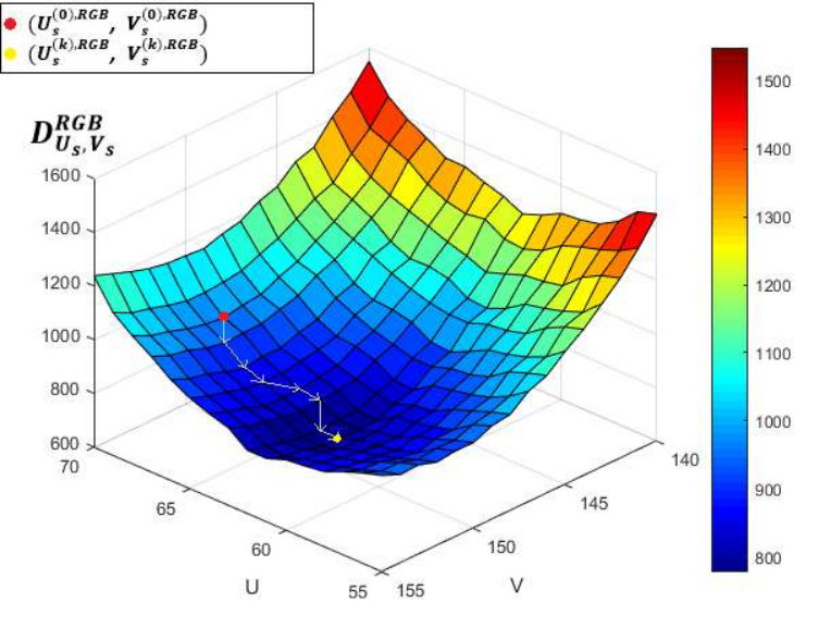
We now discuss the shape similarity between the convex block-distortion function in real domain and that in the integer domain [0, 255] [0, 255]. Under the integer domain [0, 255] [0, 255], the discretely convex-like grid plot of Fig. 5(d) is depicted in Fig. 6. In Fig. 6, the room to better improve the initial chroma subsampling solution in which the superscript “0” denotes the initial step, is indicated by the path from the red point to the yellow point in which the superscript “” denotes the th step of our iterative chroma subsampling method which will be presented in Subsection 3.2.2. Our iterative chroma subsampling method can result in less 22 RGB full-color block-distortion value, and can achieve better reconstructed RGB full-color images.
In fact, besides the 22 RGB full-color block , the shape similarity between the convex block-distortion function in real domain and that in integer domain [0, 255] [0, 255] and the room to better improve the initial chroma subsampling solution are also feasible to the 22 Bayer CFA block and the 22 DTDI CFA block .
3.2.2 Our Iterative Chroma Subsampling Procedure
As shown in Fig. 6, from the room to better improve the initial chroma subsampling solution (see the red point in Fig. 6), we now present our iterative chroma subsampling procedure to reduce the 22 () color block-distortion value for each 22 color block , resulting in better quality of the reconstructed color images. The numerical technique used in our iterative chroma subsampling procedure for the three kinds of color images is quite similar to the gradient-descent technique. For the input () color block , taking as the initial chroma subsampling solution, our iterative chroma subsampling procedure is shown below.
Step 2: Under the integer domain [0, 255] [0, 255], we calculate all the eight neighboring color block-distortion values of , namely for . Among the eight block-distortion values, we select the subsampled -pair with the minimal block-distortion value as the candidate subsampled -pair of , namely .
Step 3: If , we stop the procedure and report as the finally subsampled -pair; otherwise, we perform and go to Step 2.
The execution codes of our Improved chroma subsampling method for the input () color image can be accessed from the website [22].
4 Experimental Results
Under the VVC reference software platform VTM-8.0, based on the Kodak and IMAX datasets, the thorough experimental results demonstrated the quality and quality-bitrate tradeoff merits of our improved chroma subsampling method, in which the execution codes can be accessed from the website in [22], for , , and relative to the comparative methods. A comparison of the execution time of the considered methods is also made.
All the considered methods are implemented on a computer with an Intel Core i7-8700 CPU 3.2 GHz and 24 GB RAM. The operating system is the Microsoft Windows 10 64-bit operating system. The program development environment is Visual C++ 2019.
4.1 Quality Merit and Time Comparison
When setting QP to zero, the PSNR, CPSNR, SSIM [20] and FSIM [21] metrics are used to show the quality merit of the reconstructed images using our improved chroma subsampling method relative to the existing methods. In these experiments, the related results are computed by passing the compression process and decompression process.
4.1.1 For
The CPSNR metric of the reconstructed RGB full-color image is defined by
| (10) |
with in which the test image is of size WxH. and denote the C-color pixel-values at position in the th input RGB full-color image and the reconstructed analogue, respectively. denotes the number of testing images in the dataset. Here, is equal to 24 and 18 for the Kodak dataset and the IMAX dataset, respectively. We first calculate the CPSNR value of each dataset, and then calculate the average CPSNR value of the three related CPSNR values.
Based on the two datasets for , Table 1 indicates that our method has the highest CPSNR in boldface among the considered seven methods. The average CPSNR gains of our method are 1.9800 dB, 1.1918 dB, 2.0327 dB, 0.8019 dB, 1.1756 dB, and 0.9042 dB over 4:2:0(A), 4:2:0(L), 4:2:0(R), 4:2:0(DIRECT), 4:2:0(MPEG-B), and the IDID method [9], respectively, using the bilinear interpolation-based chroma upsampling process at the client side. Furthermore, using the bicubic interpolation-based chroma upsampling process at the client side, the average CPSNR values of the considered methods are listed in parentheses in Table 1, and our method still has the highest CPSNR in boldface. For each image, the average execution time requirement (in seconds) of each concerned method is tabulated in the last row of Table 1. Although our method takes more time than the five traditional methods in CS, our method has quality merit. When compared with IDID [9], our method takes much less time and has higher CPSNR.
Table 2 demonstrates the average CPSNR merit of our method relative to the MCIM method [10]. The average CPSNR gain of our method is 0.6046 dB over the MCIM method using the bilinear interpolation-based chroma upsampling process at the client side. In addition, using the bicubic interpolation-based chroma upsampling process, our method also still has higher CPSNR value, as listed in parenthesis in Table 2. When compared with MCIM, our method takes much less time.
SSIM is used to measure the product of the luminance, contrast, and structure similarity preserving effect between the original image and the reconstructed image. For , the SSIM value is measured by the mean of the three SSIM values for the R, G, and B color planes. FSIM is a good image quality assessment with high consistency with the subjective evaluation. FSIM first utilizes the primary feature “phase congruency (PC)” which is contrast invariant and the minor feature “gradient magnitude” to obtain the local quality map, and then FSIM utilizes PC as a weighting function to obtain a quality score.
4.1.2 For
Since the Kodak and IMAX datasets are obtained by scanning the films, each scanned RGB full-color image can be taken as a ground truth RGB full-color image. Therefore, the datasets used for are created from the two datasets. The PSNR, SSIM, and FSIM values are used to compare the quality of the reconstructed Bayer CFA images among the considered methods.Here, the reconstructed Bayer CFA images can be viewed as gray images when we measure their PSNR, SSIM, and FSIM values.
In Table 3, “BILI” denotes the bilinear interpolation-based chroma upsampling process used at the client side, and we consider the best combinations for the three comparative chroma subsampling methods, namely 4:2:0(A), the DI method [14], and the GD method [15]. Table 3 indicates that the PSNR gains of our combination, which denotes the combination “our method-BILI", over 4:2:0(A)-BILI, DI-COPY [14], and GD-BILI [15] are 6.4080 dB, 2.9973 dB, and 1.3114 dB, respectively. Table 3 also indicates that our combination has the highest SSIM and FSIM in boldface relative to the three comparative combinations.
4.1.3 For
The DTDI CFA images are collected from the two same datasets. At the client side, under the BILI based chroma upsampling process, to compare the quality performance among the three considered methods, namely 4:2:0(A), the CD method [16], and our method, the three quality metrics, CPSNR, SSIM, and FSIM, are used to measure the quality of the reconstructed DTDI images. Table 4 indicates that our method has the highest CPSNR, SSIM, and FSIM in boldface among the three considered methods, while the CD method is the fastest. In particular, the CPSNR gains of our method over 4:2:0(A) and the CD method are 2.1959 dB and 0.9459 dB, respectively.


4.2 Quality-bitrate Tradeoff Merit
When setting QP = 0, 4, 8, 12, 16, 20, 24, 28, 32, 36, 40, 44, 48, and 51, the quality-bitrate tradeoff merit of our method for , , and is depicted by the RD (rate-distortion) curves for the reconstructed RGB full-color, Bayer CFA, and DTDI CFA images, respectively. The bitrate of one compressed test set is defined by
| (11) |
where denotes the total number of bits required in compressing the test images.
For , the RD curves corresponding to the Kodak dataset and the IMAX dataset are shown in Fig. 7(a) and Fig. 7(b), respectively, in which the X-axis denotes the average bitrate required and the Y-axis denotes the average CPSNR value of the reconstructed RGB full-color images, indicating that under the same bitrate, our method has the highest CPSNR among the considered methods.
For and , the RD curves corresponding to the Kodak and IMAX datasets are depicted in Figs. 8(a)-(b) and Figs. 9(a)-(b), respectively, indicating that under the same bitrate, our method has the best quality relative to the existing methods.


| 4:2:0(A) | CD [16] | Our method | |
|---|---|---|---|
| CPSNR(dB) | 44.2594 | 45.5094 | 46.4553 |
| CPSNR Gain(dB) | 2.1959 | 0.9459 | |
| SSIM (dB) | 0.9939 | 0.9957 | 0.9966 |
| SSIM Gain (dB) | 0.0027 | 0.0009 | |
| FSIM (dB) | 0.99953 | 0.99945 | 0.99966 |
| FSIM Gain (dB) | 0.00013 | 0.00020 | |
| Execution Time(s) | 0.0013 | 0.0008 | 0.0291 |
5 Discussion and Concluding Remarks
We have presented our improved chroma subsampling method for , , and . First, we propose an improved 22 () color block-distortion function, and then we prove the convex property of our improved color block-distortion function. Next, using the differentiation technique in real domain, the closed form of the initially subsampled -pair of each 22 chroma block is derived. Furthemore, based on the shape similarity between the convex block-distortion function in real domain and that in the integer domain [0, 255] [0, 255], we propose a gradient descent-based iterative method to better improve the subsampled -pair of . Based on the Kodak and IMAX datasets, the comprehensive experimental results have justified the quality and quality-bitrate tradeoff merits of our improved chroma subsampling method for the above-mentioned three kinds of images relative to the existing traditional and state-of-the-art chroma subsampling methods. In fact, given a color image (), after performing our improved chroma subsampling method for , we can also apply the chroma subsampling-first luma modification method [23] to further improve the quality of the reconstructed color images.
There are two research issues to be studied in the future. In the first future work, besides the BILI-based chroma upsampling process used to estimate the four -pairs of , which are deployed into our improved 22 block-distortion function at the server side, we hope to extend our current BILI-based chroma upsampling approach to the other nonlinear upsampling process to better improve the quality of the reconstructed color images.
In the second future work, we hope to deploy our improved chroma subsampling method into the adaptive chroma subsampling-binding and luma-guided (ASBLG) chroma upsampling method [24] at the client side, achieving better quality of the reconstructed screen content images. However, because the subsampling position of our improved chroma subsampling method is exactly the same position as 4:2:0(A), it is very difficult to distinguish our improved method from 4:2:0(A) when using the winner-first voting strategy [24] at the client side to conclude the accurate correlation between the subsampled decoded luma image and decoded subsampled chroma image. We also put it into the future work.
Appendix A THE PROOF OF PROPOSITION 1.
Without loss of generality, we only derive Eq. (3) for the estimated U component of , namely . As depicted in Fig. 4, we assume that the coordinates of the three reference-known subsampled U components, namely , , and , are at the locations (1, 1), (0, 1), and (0, 0), respectively. Therefore, is located at (3/4, 1/4); the coordinate of the reference-unknown subsampled U component of , namely , is located at (1, 0). Applying the bilinear interpolation on the four reference U components to estimate , it yields
| (12) | ||||
Following the above derivation, we can also derive Eq. (3) for the other three estimated U components of , namely , , and . We complete the proof.
Appendix B THE PROOF OF PROPOSITION 2.
According to the quadratic convex function definition [25], if a quadratic function is positive definite, it is called a convex function. Therefore, we prove Proposition 2 by proving that our quadratic 22 () color block-distortion function in Eq. (7) is positive definite. If so, the quadratic function is called a convex function.
To prove the positive definite property of , alternately, we prove that the determinant of the Hessian matrix of , denoted by , is positive [25]. First, the Hessian matrix of is expressed by
| (13) |
with
| (14) | ||||
Furthermore, the determinant of is expressed as
| (15) | ||||
According to Eq. (15), we now prove that the value of , , is always positive for the considered three kinds of images. Considering = “”, by Eq. (15) and Eq. (6), it yields
| (16) | ||||
We have proved that the value of is positive. On the other hand, the block-distortion function is a convex function. Next, we consider = “DTDI”, by Eq. (15), it yields
| (17) | ||||
We have proved that , and it indicates that our block-distortion function is also a convex function. When = “”, by Eq. (15), it can be proved that , indicating the convex property of ; for reducing the paper length, we omit the detailed proof for it. We complete the proof.
Acknowledgments
This work was supported by the contracts MOST---E---MY and MOST---E---MY of Ministry of Science and Technology, Taiwan. The authors appreciate the proofreading help of Ms. C. Harrington to improve the manuscript.
References
- [1] Bryce E Bayer. Color imaging array, July 20 1976. US Patent 3,971,065.
- [2] Ernst Bodenstorfer, Johannes Fürtler, Jörg Brodersen, Konrad J Mayer, Christian Eckel, Klaus Gravogl, and Herbert Nachtnebel. High-speed line-scan camera with digital time delay integration. In Real-Time Image Processing 2007, volume 6496, page 64960I. International Society for Optics and Photonics, 2007.
- [3] Lei Zhang, Xiaolin Wu, Antoni Buades, and Xin Li. Color demosaicking by local directional interpolation and nonlocal adaptive thresholding. Journal of Electronic imaging, 20(2):023016, 2011.
- [4] Daisuke Kiku, Yusuke Monno, Masayuki Tanaka, and Masatoshi Okutomi. Residual interpolation for color image demosaicking. In 2013 IEEE International Conference on Image Processing, pages 2304–2308. IEEE, 2013.
- [5] Xin Li, Bahadir Gunturk, and Lei Zhang. Image demosaicing: A systematic survey. In Visual Communications and Image Processing 2008, volume 6822, page 68221J. International Society for Optics and Photonics, 2008.
- [6] DTDI Demosaicing Execution code, 2020.
- [7] RECOMMENDATION ITU-R BT et al. Studio encoding parameters of digital television for standard 4: 3 and wide-screen 16: 9 aspect ratios. 2011.
- [8] Justin Ridge and Marta Karczewicz. Joint Video Team (JVT) of ISO/IEC MPEG & ITU-T VCEG (ISO/IEC JTC1/SC29/WG11 and ITU-T SG16 Q. 6). 2007.
- [9] Yongbing Zhang, Debin Zhao, Jian Zhang, Ruiqin Xiong, and Wen Gao. Interpolation-dependent image downsampling. IEEE Transactions on Image Processing, 20(11):3291–3296, 2011.
- [10] Shiqi Wang, Ke Gu, Siwei Ma, and Wen Gao. Joint chroma downsampling and upsampling for screen content image. IEEE Transactions on Circuits and Systems for Video Technology, 26(9):1595–1609, 2015.
- [11] Xin Li and Michael T Orchard. New edge-directed interpolation. IEEE transactions on image processing, 10(10):1521–1527, 2001.
- [12] Yan Lu, Shipeng Li, and Huifeng Shen. Virtualized screen: A third element for cloud–mobile convergence. Ieee Multimedia, 18(2):4–11, 2011.
- [13] Hu Chen, Mingzhe Sun, and Eckehard Steinbach. Compression of Bayer-pattern video sequences using adjusted chroma subsampling. IEEE Transactions on Circuits and Systems for Video Technology, 19(12):1891–1896, 2009.
- [14] Chien-Hsiung Lin, Kuo-Liang Chung, and Chun-Wei Yu. Novel chroma subsampling strategy based on mathematical optimization for compressing mosaic videos with arbitrary RGB color filter arrays in H. 264/AVC and HEVC. IEEE Transactions on Circuits and Systems for Video Technology, 26(9):1722–1733, 2015.
- [15] Kuo-Liang Chung, Yu-Ling Lee, and Wei-Che Chien. Effective gradient descent-based chroma subsampling method for Bayer CFA images in HEVC. IEEE Transactions on Circuits and Systems for Video Technology, 29(11):3281–3290, 2018.
- [16] Kuo-Liang Chung, Wei-Jen Yang, Chyou-Hwa Chen, Hong-Yuan M Liao, and Sheng-Mao Zeng. Efficient chroma subsampling strategy for compressing digital time delay integration mosaic video sequences in H. 264/AVC. Journal of Electronic Imaging, 20(2):023011, 2011.
- [17] Kodak True Color Image Collection, 2014.
- [18] IMAX True Color Image Collection, 2014.
- [19] VTM-8.0, 2020.
- [20] Wang Zhou. Image quality assessment: from error measurement to structural similarity. IEEE transactions on image processing, 13:600–613, 2004.
- [21] Lin Zhang, Lei Zhang, Xuanqin Mou, and David Zhang. FSIM: A feature similarity index for image quality assessment. IEEE transactions on Image Processing, 20(8):2378–2386, 2011.
- [22] Our Method Execution code, 2020.
- [23] Kuo-Liang Chung, Tsu-Chun Hsu, and Chi-Chao Huang. Joint chroma subsampling and distortion-minimization-based luma modification for rgb color images with application. IEEE Transactions on Image Processing, 26(10):4626–4638, 2017.
- [24] Kuo-Liang Chung, Chi-Chao Huang, and Tsu-Chun Hsu. Adaptive chroma subsampling-binding and luma-guided chroma reconstruction method for screen content images. IEEE Transactions on Image Processing, 26(12):6034–6045, 2017.
- [25] Ken Binmore and Joan Davies. Calculus: concepts and methods. Cambridge University Press, 2001.
References
- [1] Bryce E Bayer. Color imaging array, July 20 1976. US Patent 3,971,065.
- [2] Ernst Bodenstorfer, Johannes Fürtler, Jörg Brodersen, Konrad J Mayer, Christian Eckel, Klaus Gravogl, and Herbert Nachtnebel. High-speed line-scan camera with digital time delay integration. In Real-Time Image Processing 2007, volume 6496, page 64960I. International Society for Optics and Photonics, 2007.
- [3] Lei Zhang, Xiaolin Wu, Antoni Buades, and Xin Li. Color demosaicking by local directional interpolation and nonlocal adaptive thresholding. Journal of Electronic imaging, 20(2):023016, 2011.
- [4] Daisuke Kiku, Yusuke Monno, Masayuki Tanaka, and Masatoshi Okutomi. Residual interpolation for color image demosaicking. In 2013 IEEE International Conference on Image Processing, pages 2304–2308. IEEE, 2013.
- [5] Xin Li, Bahadir Gunturk, and Lei Zhang. Image demosaicing: A systematic survey. In Visual Communications and Image Processing 2008, volume 6822, page 68221J. International Society for Optics and Photonics, 2008.
- [6] DTDI Demosaicing Execution code, 2020.
- [7] RECOMMENDATION ITU-R BT et al. Studio encoding parameters of digital television for standard 4: 3 and wide-screen 16: 9 aspect ratios. 2011.
- [8] Justin Ridge and Marta Karczewicz. Joint Video Team (JVT) of ISO/IEC MPEG & ITU-T VCEG (ISO/IEC JTC1/SC29/WG11 and ITU-T SG16 Q. 6). 2007.
- [9] Yongbing Zhang, Debin Zhao, Jian Zhang, Ruiqin Xiong, and Wen Gao. Interpolation-dependent image downsampling. IEEE Transactions on Image Processing, 20(11):3291–3296, 2011.
- [10] Shiqi Wang, Ke Gu, Siwei Ma, and Wen Gao. Joint chroma downsampling and upsampling for screen content image. IEEE Transactions on Circuits and Systems for Video Technology, 26(9):1595–1609, 2015.
- [11] Xin Li and Michael T Orchard. New edge-directed interpolation. IEEE transactions on image processing, 10(10):1521–1527, 2001.
- [12] Yan Lu, Shipeng Li, and Huifeng Shen. Virtualized screen: A third element for cloud–mobile convergence. Ieee Multimedia, 18(2):4–11, 2011.
- [13] Hu Chen, Mingzhe Sun, and Eckehard Steinbach. Compression of Bayer-pattern video sequences using adjusted chroma subsampling. IEEE Transactions on Circuits and Systems for Video Technology, 19(12):1891–1896, 2009.
- [14] Chien-Hsiung Lin, Kuo-Liang Chung, and Chun-Wei Yu. Novel chroma subsampling strategy based on mathematical optimization for compressing mosaic videos with arbitrary RGB color filter arrays in H. 264/AVC and HEVC. IEEE Transactions on Circuits and Systems for Video Technology, 26(9):1722–1733, 2015.
- [15] Kuo-Liang Chung, Yu-Ling Lee, and Wei-Che Chien. Effective gradient descent-based chroma subsampling method for Bayer CFA images in HEVC. IEEE Transactions on Circuits and Systems for Video Technology, 29(11):3281–3290, 2018.
- [16] Kuo-Liang Chung, Wei-Jen Yang, Chyou-Hwa Chen, Hong-Yuan M Liao, and Sheng-Mao Zeng. Efficient chroma subsampling strategy for compressing digital time delay integration mosaic video sequences in H. 264/AVC. Journal of Electronic Imaging, 20(2):023011, 2011.
- [17] Kodak True Color Image Collection, 2014.
- [18] IMAX True Color Image Collection, 2014.
- [19] VTM-8.0, 2020.
- [20] Wang Zhou. Image quality assessment: from error measurement to structural similarity. IEEE transactions on image processing, 13:600–613, 2004.
- [21] Lin Zhang, Lei Zhang, Xuanqin Mou, and David Zhang. FSIM: A feature similarity index for image quality assessment. IEEE transactions on Image Processing, 20(8):2378–2386, 2011.
- [22] Our Method Execution code, 2020.
- [23] Kuo-Liang Chung, Tsu-Chun Hsu, and Chi-Chao Huang. Joint chroma subsampling and distortion-minimization-based luma modification for rgb color images with application. IEEE Transactions on Image Processing, 26(10):4626–4638, 2017.
- [24] Kuo-Liang Chung, Chi-Chao Huang, and Tsu-Chun Hsu. Adaptive chroma subsampling-binding and luma-guided chroma reconstruction method for screen content images. IEEE Transactions on Image Processing, 26(12):6034–6045, 2017.
- [25] Ken Binmore and Joan Davies. Calculus: concepts and methods. Cambridge University Press, 2001.