跳到论文正文
W Papers独立论文阅读器 arXiv:2009.10833 论文正文 计算阅读时间 · 0%
引用这篇论文根据当前论文元数据生成,正式投稿前建议核对。


License: arXiv.org perpetual non-exclusive license
arXiv:2009.10833v1 [math.PR] 22 Sep 2020

The limiting spectral measure for an ensemble of generalized checkerboard matricesThanks: The authors were partially supported by NSF Grants DMS1947438 and DMS1561945, the University of Michigan, the University of Notre Dame, Pomona College and Williams College. We thank the authors of [BCDHMSTPY], especially Roger Van Peski, for some helpful conversations and Akihiro Takigawa for the help on programming.

Fangu Chen Email address: fangu@umich.edu Address: Department of Mathematics, University of Michigan, Ann Arbor, MI 48109 , Yuxin Lin Email address: ylin9@nd.edu Address: Department of Mathematics, University of Notre Dame, Notre Dame, IN 46556 , Steven J. Miller Email address: sjm1@williams.edu,Steven.Miller.MC.96@aya.yale.edu Address: Department of Mathematics and Statistics, Williams College, Williamstown, MA 01267 and Jiahui Yu Email address: jyad2018@mymail.pomona.edu Address: Department of Mathematics, Pomona College, Claremont, CA 91711
Date: August 11, 2026
Abstract.

Random matrix theory successfully models many systems, from the energy levels of heavy nuclei to zeros of LL-functions. While most ensembles studied have continuous spectral distribution, Burkhardt et al introduced the ensemble of kk-checkerboard matrices, a variation of Wigner matrices with entries in generalized checkerboard patterns fixed and constant. In this family, N−kN-k of the eigenvalues are of size O⁡(N)O(\sqrt{N}) and were called bulk while the rest are tightly contrained around a multiple of NN and were called blip.

We extend their work by allowing the fixed entries to take different constant values. We can construct ensembles with blip eigenvalues at any multiples of NN we want with any multiplicity (thus we can have the blips occur at sequences such as the primes or the Fibonaccis). The presence of multiple blips creates technical challenges to separate them and to look at only one blip at a time. We overcome this by choosing a suitable weight function which allows us to localize at each blip, and then exploiting cancellation to deal with the resulting combinatorics to determine the average moments of the ensemble; we then apply standard methods from probability to prove that almost surely the limiting distributions of the matrices converge to the average behavior as the matrix size tends to infinity. For blips with just one eigenvalue in the limit we have convergence to a Dirac delta spike, while if there are kk eigenvalues in a blip we again obtain hollow k×kk\times k GOE behavior.

Key words and phrases: 
Random Matrix Ensembles, Checkerboard Matrices, Limiting Spectral Measure, Gaussian Orthogonal Ensemble
2010 Mathematics Subject Classification
15B52 (primary), 15B57, 15B33 (secondary)

1. Introduction

1.1. Background

Initially introduced by Wishart [Wis] for some problems in statistics, random matrix theory has successfully modeled a large number of systems from energy levels of heavy nuclei to zeros of the Riemann zeta function; see for example the surveys [Bai, BFMT-B, Con, FM, KaSa, KeSn] and the textbooks [Fo, Meh, MT-B, Tao2]. A simple but important example is the ensemble of real symmetric matrices whose upper triangular entries are independent, identically distributed random variables from some fixed probability distribution with mean 00, variance 11 and finite higher moments. Wigner’s semi-circle law states that as the size of the matrix N→∞N\to\infty, the properly normalized spectral distribution of a matrix from the ensemble converges almost surely to a semi-circle (or semi-ellipse):

σR​(x)={2π​R2​R2−x2if ​|x|≤R,0if ​|x|>R.\sigma_{R}(x)=\begin{cases}\frac{2}{\pi R^{2}}\sqrt{R^{2}-x^{2}}&\text{{\rm if} }|x|\leq R,\\ 0&\text{{\rm if} }|x|>R.\end{cases} (1.1)

See [Wig1, Wig2, Wig3, Wig4, Wig5] for more details.

Besides the more well-known families such as the Gaussian Orthogonal, Unitary and Symplectic Ensembles, many other special ensembles have been studied; see for example [Bai, BasBo1, BasBo2, BanBo, BLMST, BCG, BHS1, BHS2, BM, BDJ, GKMN, HM, JMRR, JMP, Kar, KKMSX, LW, MMS, MNS, MSTW, McK, Me, Sch], where the additional structures on the entries of the matrices lead to different behaviors of the eigenvalues in the limit.

For most ensembles that people have studied, while it is possible to prove the convergence of the limiting spectral measure, in only a few (such as dd-regular graphs [McK], block circulant matrices [KKMSX] and palindromic Toeplitz matrices [MMS]) can the limiting distribution be written down in a nice, closed form expression.

This paper is a sequel to [BCDHMSTPY], where they introduce ensembles of checkerboard matrices which also have a nice, closed-form expression for its limiting distribution. The spectrum splits into two; most of the eigenvalues are in the bulk and are of size N\sqrt{N}, but a small number are of size NN. They studied the splitting behavior of the ensemble similar to that in [CDF1, CDF2], and used the combinatorial method in the style of [KKMSX, MMS]. The ensemble in [BCDHMSTPY] is defined as follows in the real symmetric case.

Definition 1.1.

Fix k∈ℕk\in\mathbb{N} and w∈ℝw\in\mathbb{R}. The N×NN\times N (k,w)(k,w)-checkerboard ensemble over ℝ\mathbb{R} is the ensemble of matrices M=(mi​j)M=(m_{ij}) given by

mi​j={ai​jif ​i≢jmodkwif ​i≡jmodk,m_{ij}\ =\ \begin{cases}a_{ij}&\text{{\rm if} }i\not\equiv j\bmod k\\ w&\text{{\rm if} }i\equiv j\bmod k,\end{cases} (1.2)

where ai​j=aj​ia_{ij}=a_{ji} are i.i.d. random variables with mean 0, variance 1, and finite higher moments, and the probability measure on the ensemble given by the natural product probability measure.

For this ensemble N−kN-k of the eigenvalues (called the bulk eigenvalues) are of order N\sqrt{N} and converge to a semi-circle, while kk of the eigenvalues (called the blip eigenvalues) are of order NN and converge to the spectral distribution of a k×kk\times k hollow Gaussian orthogonal ensemble.

Definition 1.2.

The k×kk\times k hollow Gaussian Orthogonal Ensemble is given by k×kk\times k matrices A=(ai​j)=ATA=(a_{ij})=A^{T} with

ai​j={𝒩ℝ​(0,1)if ​i≠j0if ​i=j.a_{ij}=\begin{cases}\mathcal{N}_{\mathbb{R}}(0,1)&\text{{\rm if} }i\neq j\\ 0&\text{{\rm if} }i=j.\end{cases} (1.3)

See [BCDHMSTPY] for a collection of histograms of eigenvalues of matrices from some k×kk\times k hollow GOE.

1.2. Generalized Checkerboard Ensembles

We generalize [BCDHMSTPY] by allowing the constant ww to take different values. While the Checkerboard ensembles in [BCDHMSTPY] only allow one blip for each ensmble, the generalized Checkerboard ensembles allow arbitrarily many blips for each ensemble. Moreover, we have control over the positions of these blips. That is, given a list of points, the generalized checkerboard ensemble allows the spectrum at those points in a “non-trivial” way. We can always “trivially” construct ensembles with prescribed locations and frequency by taking a diagonal union of block matrices. But then the blocks are independent from each other. The significance of the generalized checkerboard ensemble is that we can control the locations of normalized eigenvalues within an ensemble that doesn’t have independent diagonal blocks. It is a "mixed" matrix whose eigenvalues have a nice split limiting distribution.

Definition 1.3.

Fix k∈ℕk\in\mathbb{N} and a kk-tuple of real numbers W=(w1,…,wk)W=(w_{1},\dots,w_{k}), then the N×NN\times N (k,W)(k,W)-checkerboard ensemble is the ensemble of matrices AN=(mi​j)A_{N}=(m_{ij}) given by

mi​j={ai​j if ​i≢j(modk),wu if i≡j≡u(modk), with u∈{1,2,…,k},\displaystyle m_{ij}\;=\;\begin{cases}a_{ij}&\text{ if }i\not\equiv j\pmod{k},\\ w_{u}&\text{ if }i\equiv j\equiv u\pmod{k},\text{ with }u\in\{1,2,\dots,k\},\end{cases} (1.4)

where ai​j=aj​ia_{ij}=a_{ji} are independent and identically distributed random variables with mean 00, variance 11, and finite higher moments.

For example, when k=3k=3, W=(1,1,2)W=(1,1,2), a (3,W)(3,W) checkerboard looks like the following (we assume 3|N3|N):

X=(1a12a131a15a16…1a1​N−1a1​Na121a23a241a26…a2​N−21a2​Na13a232a34a352…a3​N−2a3​N−12⋱a1​Na2​N2a4​Na5​N2…aN−2​NaN−1​N2).X=\begin{pmatrix}1&a_{12}&a_{13}&1&a_{15}&a_{16}&\dots&1&a_{1N-1}&a_{1N}\\ a_{12}&1&a_{23}&a_{24}&1&a_{26}&\dots&a_{2N-2}&1&a_{2N}\\ a_{13}&a_{23}&2&a_{34}&a_{35}&2&\dots&a_{3N-2}&a_{3N-1}&2\\ \vdots&\vdots&\vdots&\vdots&\vdots&\vdots&\ddots&\vdots&\vdots&\vdots\\ a_{1N}&a_{2N}&2&a_{4N}&a_{5N}&2&\dots&a_{N-2N}&a_{N-1N}&2\\ \end{pmatrix}.

1.3. Results

What makes the checkerboard ensemble in [BCDHMSTPY] interesting is that the eigenvalues of a matrix from the ensemble almost surely fall into two separate regimes. With our generalization we can exploit the freedom to choose different constants to force the eigenvalues to fall into more regimes. To be more precise, using matrix perturbation theory we prove the following result.

Theorem 1.4.

Let {AN}N∈ℕ\{A_{N}\}_{N\in\mathbb{N}} be a sequence of (k,W)(k,W)-checkerboard matrices. Suppose that WW has xx non-zero entries and there are ss distinct ww’s, then almost surely as N→∞N\rightarrow\infty, the eigenvalues of ANA_{N} fall into s+1s+1 regimes: N−xN-x of the eigenvalues are O⁡(N1/2+ϵ)O(N^{1/2+\epsilon}) and if wi′w_{i}^{\prime} appears kik_{i} times, kik_{i} eigenvalues are of magnitude N​wi′/k+O⁡(N1/2+ϵ)Nw_{i}^{\prime}/k+O(N^{1/2+\epsilon}).

As in [BCDHMSTPY], we refer to the N−xN-x eigenvalues that are on the order of N\sqrt{N} as the eigenvalues in the bulk, while for each distinct wiw_{i}, the kik_{i} eigenvalues near N​wi/kNw_{i}/k are called the eigenvalues in the blips. We study the eigenvalue distribution of each regime.

For the remainder of this paper, 𝑨𝑵\boldsymbol{A_{N}} always refers to an N×NN\times N matrix.

Let νAN\nu_{A_{N}} be the empirical spectral measure of an N×NN\times N matrix ANA_{N}, where we have normalized the eigenvalues by dividing by N\sqrt{N}:

νAN​(x)=1N​∑λ​ an eigenvalue of ​ANδ⁡(x−λN).\nu_{A_{N}}(x)\ =\ \frac{1}{N}\sum_{\lambda\text{ \rm an eigenvalue of }A_{N}}\delta\left(x-\frac{\lambda}{\sqrt{N}}\right). (1.5)

For example, Figure 1 gives this normalized eigenvalue distribution of a collection of 500×500500\times 500 (6,W)(6,W)-checkerboard matrices with W=(1,−2,−2,3,3,3)W=(1,-2,-2,3,3,3).

Refer to caption
Figure 1. A histogram of the normalized eigenvalue distribution on a probability density scale for 500×500500\times 500 (6,W)(6,W)-checkerboard real matrices with W=(1,−2,−2,3,3,3)W=(1,-2,-2,3,3,3) after 500 trials.

As in [BCDHMSTPY], the blip eigenvalues of order NN prevent us from directly using the method of moments (for large mm, the contribution from these eigenvalues dwarfs that from the bulk). We use following result (see [Tao1]) to bypass the complications presented by the small number of blip eigenvalues.

Proposition 1.5.

([Tao1]) Let {𝒜N}N∈ℕ\{\mathcal{A}_{N}\}_{N\in\mathbb{N}} be a sequence of random Hermitian matrix ensembles such that {ν𝒜N,N}N∈ℕ\{\nu_{\mathcal{A}_{N},N}\}_{N\in\mathbb{N}} converges weakly almost surely to a limit ν\nu. Let {𝒜~N}N∈ℕ\{\tilde{\mathcal{A}}_{N}\}_{N\in\mathbb{N}} be another sequence of random matrix ensembles such that 1N​rank⁡(𝒜~N)\frac{1}{N}\rank(\tilde{\mathcal{A}}_{N}) converges almost surely to zero. Then {ν𝒜N+𝒜~N,N}N∈ℕ\{\nu_{\mathcal{A}_{N}+\tilde{\mathcal{A}}_{N},N}\}_{N\in\mathbb{N}} converges weakly almost surely to ν\nu.

Taking 𝒜~N\tilde{\mathcal{A}}_{N} to be the fixed matrix with entries mi​j=wum_{ij}=w_{u} whenever i≡j≡u(modk)i\equiv j\equiv u\pmod{k} and zero otherwise, we have that the limiting spectral distribution of the (k,W)(k,W)-checkerboard ensemble is the same as the limiting spectral distribution of the ensemble with W=𝟎W=\mathbf{0}, which does not have the kk large blip eigenvalues . This overcomes the issue of diverging moments.

Theorem 1.6.

Let {AN}N∈ℕ\{A_{N}\}_{N\in\mathbb{N}} be a sequence of N×NN\times N (k,W)(k,W)-checkerboard matrices, and let νAN\nu_{A_{N}} denote the empirical spectral measure, then νAN\nu_{A_{N}} converges weakly almost surely to the Wigner semicircle measure σR\sigma_{R} with radius

R= 2​1−1/k.R\ =\ 2\sqrt{1-1/k}. (1.6)

The proof is by standard combinatorial arguments. We give the details in §2.1.

Similar to the previous checkerboard paper [BCDHMSTPY], each blip may be thought of as deviations about the trivial eigenvalues. Instead of having just one blip as in [BCDHMSTPY], we now have many different blips. A blip containing ki>1k_{i}>1 eigenvalues has the same distribution as the eigenvalues of the ki×kik_{i}\times k_{i} hollow Gaussian Orthogonal Ensemble (see Definition 1.2); when ki=1k_{i}=1 the blip has the distribution of a dirac delta function.

We need to define a weighted blip spectral measure which takes into account only the eigenvalues of one blip. Thus we not only need to get rid of the interference from the bulk, we also need to avoid the interference from the other blips. In order to facilitate the use of eigenvalue trace lemma, similar to [BCDHMSTPY], we are led to use a polynomial weighting function and we use a sequence of polynomials of degree tending to infinity as the matrix size N→∞N\rightarrow\infty so that in the limit we mimic a smooth cutoff function. Specifically, let

fi2​n​(x):=(x⁡(2−x)​∏wj≠wi(x−wjwi)​(2−x−wjwi)∏wj≠wi(1−wjwi)2)2​n.f_{i}^{2n}(x)\;:=\;\left(\frac{x(2-x)\prod_{w_{j}\neq w_{i}}(x-\frac{w_{j}}{w_{i}})(2-x-\frac{w_{j}}{w_{i}})}{\prod_{w_{j}\neq w_{i}}(1-\frac{w_{j}}{w_{i}})^{2}}\right)^{2n}. (1.7)

Thus we alter the standard empirical spectral measure in the following way to capture the blip. For example, when k=3k=3 and W=(1,1,2)W=(1,1,2), we use the polynomial f32​n​(x)=(x⁡(2−x)​(2​x−1)​(3−2​x))2​nf_{3}^{2n}(x)=\left(x(2-x)(2x-1)(3-2x)\right)^{2n} to study the blip around 2​N3\frac{2N}{3}. Figure 2 gives a plot of the polynomial f3200​(x)f_{3}^{200}(x). We can see that the weight function f32​n​(x)f_{3}^{2n}(x) is large when |x−1|>52|x-1|>\frac{\sqrt{5}}{2}, but this would not cause a problem since almost surely there will be no scaled eigenvalues in that region.
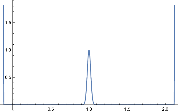
Refer to caption
Figure 2. Weight function with n=100n=100 to study the blip around 2​N3\frac{2N}{3} when k=3k=3 and W=(1,1,2)W=(1,1,2).
Definition 1.7.

Given k∈ℕk\in\mathbb{N} and a kk-tuple of real numbers W=(w1,…,wk)W=(w_{1},\dots,w_{k}), the empirical blip spectral measure associated to an N×NN\times N (k,W)(k,W)-checkerboard matrix ANA_{N} around N​wi/k≠0Nw_{i}/k\neq 0 is

μAN,i​(x):=1ki​∑λ​ an eigenvalue of ​Afi2​n​(k​λwi​N)​δ​(x−(λ−wi​Nk)),\mu_{A_{N},i}(x)\;:=\;\frac{1}{k_{i}}\sum_{\lambda\text{ \rm an eigenvalue of }A}f_{i}^{2n}\left(\frac{k\lambda}{w_{i}N}\right)\delta\left(x-\left(\lambda-\frac{w_{i}N}{k}\right)\right), (1.8)

where kik_{i} is the number of wiw_{i}’s in (w1,…,wk)(w_{1},\dots,w_{k}), and n⁡(N)n(N) is a function satisfying limN→∞n⁡(N)=∞\lim\limits_{N\to\infty}n(N)=\infty and n⁡(N)=O⁡(log⁡log⁡N)n(N)=O(\log\log N).

Remark 1.8.

The actual choice of weight functions should not change the empirical blip spectral measure in the limit. It will be used in the proof that the weight polynomial fi2​n​(x)f_{i}^{2n}(x) has a critical point at 11 with fi2​n​(1)=1f_{i}^{2n}(1)=1 and has zeroes of order 2​n2n at 00 and at all wj/w1w_{j}/w_{1} with wj≠w1w_{j}\neq w_{1}. Heuristically, because the fluctuation of eigenvalues in each regime is of order N\sqrt{N}, we have fi2​n​(k​λwi​N)≈1f_{i}^{2n}\left(\frac{k\lambda}{w_{i}N}\right)\approx 1 if λ\lambda is in the blip around N​wi/kNw_{i}/k, and fi2​n​(k​λwi​N)≈0f_{i}^{2n}\left(\frac{k\lambda}{w_{i}N}\right)\approx 0 if λ\lambda is in the bulk or in the blip other than N​wi/kNw_{i}/k. More specifically,

fi2​n​(k​λwi​N)={O⁡(log⁡NNn) if ​λ​ is ​O​(N)​ or ​N​wjk+O⁡(N)​ with ​wj≠wi,1+O⁡(log⁡NN2​n) if ​λ​ is ​N​wik+O⁡(N).\displaystyle f_{i}^{2n}\left(\frac{k\lambda}{w_{i}N}\right)\;=\;\begin{cases}O\left(\frac{\log{N}}{N^{n}}\right)&\text{ {\rm if} }\lambda\text{ {\rm is} }O\left(\sqrt{N}\right)\text{ {\rm or} }\frac{Nw_{j}}{k}+O\left(\sqrt{N}\right)\text{ {\rm with} }w_{j}\neq w_{i},\\ 1+O\left(\frac{\log{N}}{N^{2n}}\right)&\text{ {\rm if} }\lambda\text{ {\rm is} }\frac{Nw_{i}}{k}+O\left(\sqrt{N}\right).\end{cases} (1.9)

As in [BCDHMSTPY], we use the method of moments to reduce to a combinatorial problem and relate the expected moments of the empirical blip measure around N​wi/kNw_{i}/k to those of the ki×kik_{i}\times k_{i} hollow GOE. One remarkable observation is that the values of the constants wj≠wiw_{j}\neq w_{i} do not affect the blip eigenvalues around N​wi/kNw_{i}/k.

For example, if we choose W1=(1,−2,−2,3,3,3)W_{1}=(1,-2,-2,3,3,3) and W2=(0,0,0,3,3,3)W_{2}=(0,0,0,3,3,3), then numerically we can observe that the histograms (Figure 3 and 4) of the eigenvalues of the 500×500500\times 500 (6,W1)(6,W_{1})-checkerboard matrices and (6,W2)(6,W_{2})-checkerboard matrices at the blip around 1N​N⋅36=1500​500⋅36≈11.2\frac{1}{\sqrt{N}}\frac{N\cdot 3}{6}=\frac{1}{\sqrt{500}}\frac{500\cdot 3}{6}\approx 11.2 after normalization have approximately the same shape.

Refer to caption
Figure 3. A histogram of the largest blip on a probability density scale for 500×500500\times 500 (6,W1)(6,W_{1})-checkerboard real matrices with W1=(1,−2,−2,3,3,3)W_{1}=(1,-2,-2,3,3,3) after 500 trials.
Refer to caption
Figure 4. A histogram of the largest blip on a probability density scale for 500×500500\times 500 (6,W2)(6,W_{2})-checkerboard real matrices with W2=(0,0,0,3,3,3)W_{2}=(0,0,0,3,3,3) after 500 trials.

In particular, when there is only one eigenvalue in a blip, we obtain the following.

Theorem 1.9.

Fix k∈ℕk\in\mathbb{N} and a kk-tuple of real numbers W=(w1,…,wk)W=(w_{1},\dots,w_{k}) where wi≠0w_{i}\neq 0 and there is exactly one wiw_{i} in WW. Let {AN}N∈ℕ\{A_{N}\}_{N\in\mathbb{N}} be a sequence of (k,W)(k,W)-checkerboard matrices. Then the associated empirical blip spectral measure μAN,i\mu_{A_{N},i} around N​wi/kNw_{i}/k converges weakly to the Dirac delta distribution centered at N​wik+k−1wi\frac{Nw_{i}}{k}+\frac{k-1}{w_{i}}.

Thus, when ki=1k_{i}=1, we expect an eigenvalue of magnitude exactly N​wik+k−1wi\frac{Nw_{i}}{k}+\frac{k-1}{w_{i}} as N→∞N\to\infty. In general, when ki>1k_{i}>1, the empirical blip spectral measure of one matrix ANA_{N} around N​wi/kNw_{i}/k no longer converges to the expected value, as the variances of the moments do not necessarily converge to zero as N→∞N\to\infty. Thus, we follow [BCDHMSTPY] to modify the moment convergence theorem and average over the eigenvalues of multiple independent matrices.

Definition 1.10.

Fix k∈ℕk\in\mathbb{N}, a kk-tuple of real numbers W=(w1,…,wk)W=(w_{1},\dots,w_{k}), and a function g:ℕ→ℕg:\mathbb{N}\rightarrow\mathbb{N}. The averaged empirical blip spectral measure around N​wi/kNw_{i}/k associated to a g⁡(N)g(N)-tuple of N×NN\times N (k,W)(k,W)-checkerboard matrices (AN(1),AN(2),…,AN(g⁡(N)))(A_{N}^{(1)},A_{N}^{(2)},\dots,A_{N}^{(g(N))}) is

μi,g,AN(1),AN(2),…,AN(g⁡(N)):=1g⁡(N)​∑j=1g⁡(N)μAN(j),i.\mu_{i,g,A_{N}^{(1)},A_{N}^{(2)},\dots,A_{N}^{(g(N))}}\ :=\ \frac{1}{g(N)}\sum_{j=1}^{g(N)}\mu_{A_{N}^{(j)},i}. (1.10)
Theorem 1.11.

Fix k∈ℕk\in\mathbb{N}, a kk-tuple of real numbers W=(w1,…,wk)W=(w_{1},\dots,w_{k}). Let g:ℕ→ℕg:\mathbb{N}\rightarrow\mathbb{N} be such that there exists a δ>0\delta>0 for which g⁡(N)≫Nδg(N)\gg N^{\delta}. Let A(j)={AN(j)}N∈ℕA^{(j)}=\{A^{(j)}_{N}\}_{N\in\mathbb{N}} be sequences of fixed N×NN\times N matrices, and let A¯={A(j)}j∈ℕ\overline{A}=\{A^{(j)}\}_{j\in\mathbb{N}} be a sequence of such sequences. Then, as N→∞N\to\infty, the averaged empirical blip spectral measures μi,g,AN(1),AN(2),…,AN(g⁡(N))\mu_{i,g,A_{N}^{(1)},A_{N}^{(2)},\dots,A_{N}^{(g(N))}} around N​wi/kNw_{i}/k of the (k,W)(k,W)-checkerboard ensemble over ℝ\mathbb{R} converge weakly almost-surely to the measure with moments equal to the expected moments of the standard empirical spectral measure of the ki×kik_{i}\times k_{i} hollow Gaussian Orthogonal Ensemble, where kik_{i} is the number of wiw_{i} in WW.

In conclusion, we can construct an expanding family to have blips of any desired finite size at any sequence of positions after normalization. For example, we give an explicit construction of an ensemble whose limiting spectral measure has a semi-circle bulk and blips at all the Fibonacci numbers in Appendix F. Moreover, we extend [BCDHMSTPY] by showing that the averaged empirical blip spectral measure around N​wik\frac{Nw_{i}}{k} converges to a ki×kik_{i}\times k_{i} hollow Gaussian with its mean k−1wi\frac{k-1}{w_{i}} independent of the choice of all the constants wj≠wiw_{j}\neq w_{i}. This measn that the distribution of different blips don’t interfere with each other. When the blip has size ki=1k_{i}=1, we get weak convergence of empirical blip spectral measure around N​wik\frac{Nw_{i}}{k} to a Dirac Delta distribtion.

The paper is organized as follows. In §2 we prove our claims concerning the eigenvalues in the bulk, then turn to the blip spectral measure in §3. We then prove results on the convergence to the limiting spectral measure in §4.

2. The Bulk Spectral Measure and the split behavior

2.1. Bulk Measure

In this section we establish that the limiting bulk measure for the generalized kk-checkerboard matrices follows a semi-circle. We denote by μ(m)\mu^{(m)} the mmth moment of the measure μ\mu.

The commonly used method of moments cannot be directly applied to our ensemble because as proved in [BCDHMSTPY] the limiting expected moments of the empirical spectral measure do not exist. As remarked in the introduction, we overcome this difficulty by connecting the limiting spectral measure of the generalized checkerboard ensemble with that of N×N⁡(k,0)N\times N(k,0) checkerboard ensembles through Proposition 1.5. [BCDHMSTPY] then use the method of moments to establish the result for (k,0)(k,0)-checkerboard matrices, using the eigenvalue trace lemma and combinatorics to establish convergence of the expected moments. The remaining arguments establishing almost sure weak convergence are standard (see for example Appendix A of [BCDHMSTPY]); we state the result below.

Lemma 2.1.

The expected moments of the bulk empirical spectral measure taken over ANA_{N} in the N×NN\times N (k,0)(k,0)-checkerboard ensemble converge to the moments of the Wigner semicircle distribution σR\sigma_{R} as defined in (1.1) with radius R=2​1−1/kR=2\sqrt{1-1/k} and

𝔼⁡[νAN(l)]→σR(l)\mathbb{E}\left[\nu^{(l)}_{A_{N}}\right]\rightarrow\sigma_{R}^{(l)} (2.1)

as N→∞N\rightarrow\infty.

Thus, by Lemmas 2.1 and 1.5, we obtain the limiting distribution for the bulk of the general checkerboard ensemble.

Lemma 2.2.

The expected moments of the bulk empirical spectral measure taken over ANA_{N} in the N×NN\times N general (k,W)(k,W)-checkerboard ensemble converge to the moments of the Wigner semicircle distribution σR\sigma_{R} with radius R=2​1−1/kR=2\sqrt{1-1/k} and

𝔼⁡[νAN(ℓ)]→σR(ℓ)\mathbb{E}\left[\nu^{(\ell)}_{A_{N}}\right]\rightarrow\sigma_{R}^{(\ell)} (2.2)

as N→∞N\rightarrow\infty.

2.2. Split Behavior

In this section we demonstrate that general checkerboard matrices with ss different non-zero ww’s almost surely have s+1s+1 regimes of eigenvalues. One is O⁡(N1/2+ϵ)O(N^{1/2+\epsilon}) (the bulk) and the others are of order NN (the blip). Similar to Appendix B of [BCDHMSTPY], we rely on matrix perturbation theory. In particular, we view a (k,w)(k,w)-checkerboard matrix as the sum of a (k,0)(k,0)-checkerboard matrix and a fixed matrix ZZ where Zi​j=wuχ{i≡j≡umodk}Z_{ij}=w_{u}\chi\{{i\equiv j\equiv u\bmod k}\}. In that sense, we view the (k,w)(k,w)-checkerboard matrix as a perturbation of the matrix ZZ. Then, as the spectral radius of the (k,0)(k,0)-checkerboard matrix is O⁡(N1/2+ϵ)O(N^{1/2+\epsilon}), we obtain by standard results in the theory of matrix perturbations that the spectrum of the (k,w)(k,w)-checkerboard matrix is the same as that of matrix ZZ up to an order N1/2+ϵN^{1/2+\epsilon} perturbation.

We begin with the following observation on the spectrum of the matrix ZZ.

Lemma 2.3.

Suppose that WW has xx non-zero entries and suppose that wi′w^{\prime}_{i} appears kik_{i} times in W=(w1,…,wk)W=(w_{1},\dots,w_{k}), then the matrix ZZ has exactly kik_{i} eigenvalues at N​wi′/kNw^{\prime}_{i}/k and has N−xN-x eigenvalues at zero.

Proof.

Suppose wi1=wi2=⋯=wit=wi′w_{i_{1}}=w_{i_{2}}=\dots=w_{i_{t}}=w_{i^{\prime}}, then for 1≤j≤t1\leq j\leq t the vectors ∑i=0(N−1)/kek​i+ij\sum_{i=0}^{(N-1)/k}e_{ki+i_{j}} are eigenvectors with eigenvalues N​wi′/kNw_{i^{\prime}}/k. Furthermore, for 1≤i≤N1\leq i\leq N and 1≤j<k1\leq j<k the vector ek​i+j−ek​i+j+1e_{ki+j}-e_{ki+j+1} are eigenvectors with eigenvalues equal to 00. ∎

Weyl’s inequality gives the following.

Lemma 2.4.

(Weyl’s inequality) [HJ] Let H,PH,P be N×NN\times N Hermitian matrices, and let the eigenvalues of HH, PP, and H+PH+P be arranged in increasing order. Then for every pair of integers such that 1≤j,k≤N1\leq j,k\leq N and j+k≥N+1j+k\geq N+1 we have

λj+k−N​(H+P)≤λj​(H)+λk​(P),\lambda_{j+k-N}(H+P)\ \leq\ \lambda_{j}(H)+\lambda_{k}(P), (2.3)

and for every pair of integers j,kj,k such that 1≤j,k≤N1\leq j,k\leq N and j+k≤N+1j+k\leq N+1 we have

λj​(H)+λk​(P)≤λj+k−1​(H+P).\lambda_{j}(H)+\lambda_{k}(P)\ \leq\ \lambda_{j+k-1}(H+P). (2.4)

Let ‖P‖op\|P\|_{\text{op}} denote maxi⁡|λi​(P)|\max_{i}\left|\lambda_{i}(P)\right|. By using the fact that |λk​(P)|≤‖P‖op\left|\lambda_{k}(P)\right|\leq\|P\|_{\text{op}} and taking k=Nk=N in (2.3), we obtain that λj​(H+P)≤λj​(H)+‖P‖op\lambda_{j}(H+P)\leq\lambda_{j}(H)+\|P\|_{\text{op}}. Taking k=1k=1 in (2.4) gives the inequality on the other side, hence |λj​(H+P)−λj​(H)|≤‖P‖op\left|\lambda_{j}(H+P)-\lambda_{j}(H)\right|\leq\|P\|_{\text{op}}.

The above lemma implies that if the spectral radius of PP is O⁡(f)O(f) then the size of the perturbations are O⁡(f)O(f) as well. Hence it suffices to demonstrate that almost surely the spectral radius of a sequence of (k,0)(k,0)-checkerboard matrices is O⁡(N1/2+ϵ)O(N^{1/2+\epsilon}).

Let ANA_{N} be a (k,0)(k,0)-checkerboard matrix. By Remark A.3 in [BCDHMSTPY] we have that Var​(Tr⁡(AN2​m))=O⁡(N2​m)\text{Var}(\tr(A^{2m}_{N}))=O(N^{2m}) and by the proof of Lemma 2.1 we get 𝔼⁡[Tr⁡(AN2​m)]=O⁡(Nm+1)\mathbb{E}\left[\tr(A^{2m}_{N})\right]=O(N^{m+1}).

Since Lemma B.2 in [BCDHMSTPY] holds for all m∈ℤ+m\in\mathbb{Z}^{+}, we have that almost surely ‖AN‖op\|A_{N}\|_{\text{op}} is O⁡(N1/2+ϵ)O(N^{{1/2}+\epsilon}). Together with Lemma 2.3 and Lemma 2.4, we obtain the following.

See 1.4

3. The Blip Spectral Measure

In this section, we study the distribution of the eigenvalues at the blips. First, we define a weight function to enable us to focus on just one blip at a time. Then, we reduce the general cases to the case where all wj≠wiw_{j}\not=w_{i} are zero. Finally, we show that the distribution in the special case is hollow k1×k1k_{1}\times k_{1} gaussian following an argument similar to the one in [BCDHMSTPY].

Without loss of generality, we focus on the blip around N​w1/k≠0Nw_{1}/k\neq 0 and use the polynomial weight function

f12​n​(x)=(x⁡(2−x)​∏wj≠w1(x−wjw1)​(2−x−wjw1)∏wj≠w1(1−wjw1)2)2​n.f_{1}^{2n}(x)\ =\ \left(\frac{x(2-x)\prod_{w_{j}\neq w_{1}}(x-\frac{w_{j}}{w_{1}})(2-x-\frac{w_{j}}{w_{1}})}{\prod_{w_{j}\neq w_{1}}(1-\frac{w_{j}}{w_{1}})^{2}}\right)^{2n}. (3.1)

As discussed in Remark 1.8, the particular choice of weight functions does not change the result, provided that they are essentially 11 close to 11 and vanish to sufficiently high order at 00 and all wj/w1w_{j}/w_{1} to remove the contribution from the eigenvalues within the bulk and the other blips.

Definition 3.1.

The empirical blip spectral measure associated to an N×NN\times N kk-checkerboard matrix ANA_{N} around N​w1/kNw_{1}/k is

μAN,1​(x):=1k1​∑λ​ an eigenvalue of ​Af12​n​(k​λw1​N)​δ​(x−(λ−w1​Nk)),\mu_{A_{N},1}(x)\;:=\;\frac{1}{k_{1}}\sum_{\lambda\text{ \rm an eigenvalue of }A}f_{1}^{2n}\left(\frac{k\lambda}{w_{1}N}\right)\delta\left(x-\left(\lambda-\frac{w_{1}N}{k}\right)\right), (3.2)

where k1k_{1} is the number of w1w_{1}’s in (w1,…,wk)(w_{1},\dots,w_{k}), and n⁡(N)n(N) is a function satisfying limN→∞n⁡(N)=∞\lim\limits_{N\to\infty}n(N)=\infty and n⁡(N)=O⁡(log⁡log⁡N)n(N)=O(\log\log N).

Because the fluctuation of the location of the eigenvalues in each regime is of order N\sqrt{N}, the modified spectral measure of Definition 3.1 weights eigenvalues within this blip by almost exactly 1 and those in the bulk and the other blips by almost exactly zero.

For fixed NN, the polynomial f12​nf_{1}^{2n} can be written as f12​n​(x)=∑α=2​n4​n​lcα​xαf_{1}^{2n}(x)=\displaystyle\sum_{\alpha=2n}^{4nl}c_{\alpha}x^{\alpha}, where ll is the number of distinct constants in (w1,…,wk)(w_{1},\dots,w_{k}) and all cα∈ℝc_{\alpha}\in\mathbb{R}.

We apply the method of moments to the modified spectral measure (3.2). By the eigenvalue trace formula and linearity of expectation, the expected mm-th moment of the empirical blip spectral measure is

𝔼⁡[μAN,1(m)]=\displaystyle\mathbb{E}\left[\mu_{A_{N},1}^{(m)}\right]\;=\; 𝔼⁡[1k1​∑λ∑α=2​n4​n​lcα​(k​λw1​N)α​(λ−w1​Nk)m]\displaystyle\mathbb{E}\left[\frac{1}{k_{1}}\sum_{\lambda}\sum_{\alpha=2n}^{4nl}c_{\alpha}\left(\frac{k\lambda}{w_{1}N}\right)^{\alpha}\left(\lambda-\frac{w_{1}N}{k}\right)^{m}\right]
=\displaystyle=\; 𝔼⁡[1k1​∑α=2​n4​n​lcα​(kw1​N)α​(∑i=0m(mi)​(−w1​Nk)m−i​Tr​(ANα+i))]\displaystyle\mathbb{E}\left[\frac{1}{k_{1}}\sum_{\alpha=2n}^{4nl}c_{\alpha}\left(\frac{k}{w_{1}N}\right)^{\alpha}\left(\sum_{i=0}^{m}\binom{m}{i}\left(-\frac{w_{1}N}{k}\right)^{m-i}\text{Tr}(A_{N}^{\alpha+i})\right)\right]
=\displaystyle=\; 1k1​∑α=2​n4​n​lcα​(kw1​N)α​(∑i=0m(mi)​(−w1​Nk)m−i​𝔼​[Tr​(ANα+i)]).\displaystyle\frac{1}{k_{1}}\sum_{\alpha=2n}^{4nl}c_{\alpha}\left(\frac{k}{w_{1}N}\right)^{\alpha}\left(\sum_{i=0}^{m}\binom{m}{i}\left(-\frac{w_{1}N}{k}\right)^{m-i}\mathbb{E}\left[\text{Tr}(A_{N}^{\alpha+i})\right]\right). (3.3)

Recall that

𝔼[Tr(ANα+i)]=∑1≤j1,…,jα+i≤N𝔼[mj1​j2mj2​j3⋯mjα+i​j1].\mathbb{E}\left[\text{Tr}(A_{N}^{\alpha+i})\right]\;=\;\sum_{1\leq j_{1},\ldots,j_{\alpha+i}\leq N}\mathbb{E}\left[m_{j_{1}j_{2}}m_{j_{2}j_{3}}\cdots m_{j_{\alpha+i}j_{1}}\right]. (3.4)

The calculation of the moment has been transformed into a combinatorial problem of counting different types of products of entries. We follow the vocabulary from [BCDHMSTPY] to describe the combinatorics problem.

Definition 3.2.

A block is a set of adjacent aa’s surrounded by ww’s in a cyclic product, where the last entry of a cyclic product is considered to be adjacent to the first. We refer to a block of length ℓ\ell as an ℓ\ell-block or sometimes a block of size ℓ\ell.

Definition 3.3.

A configuration is the set of all cyclic products for which it is specified (a) how many blocks there are, and of what lengths, and (b) in what order these blocks appear (up to cyclic permutation); However, it is not specified how many ww’s there are between each block.

Definition 3.4.

A congruence configuration is a configuration together with a choice of the congruence class modulo kk of every index.

Definition 3.5.

Given a configuration, a matching is an equivalence relation ∼\sim on the aa’s in the cyclic product which constrains the ways of indexing (see Definition 3.6) the aa’s as follows: an indexing of aa’s conforms to a matching ∼\sim if, for any two aa’s aiℓ,iℓ+1a_{i_{\ell},i_{\ell+1}} and ait,it+1a_{i_{t},i_{t+1}}, we have {iℓ,iℓ+1}={it,it+1}\{i_{\ell},i_{\ell+1}\}=\{i_{t},i_{t+1}\} if and only if aiℓ​iℓ+1∼ait,it+1a_{i_{\ell}i_{\ell+1}}\sim a_{i_{t},i_{t+1}}. We further constrain that each aa is matched with at least one other by any matching ∼\sim.

Definition 3.6.

Given a configuration, matching, and length of the cyclic product, then an indexing is a choice of

  1. (1)

    the (positive) number of ww’s between each pair of adjacent blocks (in the cyclic sense), and

  2. (2)

    the integer indices of each aa and ww in the cyclic product.

Example 3.7.

Consider the configuration

⋯ai1​i2wi2​i3wi3​i4ai4​i5ai5​i6⋯.\cdots a_{i_{1}i_{2}}w_{i_{2}i_{3}}w_{i_{3}i_{4}}a_{i_{4}i_{5}}a_{i_{5}i_{6}}\cdots. (3.5)

Then we have

i2≡i3≡i4(modk).i_{2}\equiv i_{3}\equiv i_{4}\pmod{k}. (3.6)

We see that the congruence classes of the indices of the aa’s determine which congruence classes of the indices of the ww’s belong to, and thus which wjw_{j}’s appear between the blocks.

3.1. Reducing to the case where all wj≠w1w_{j}\neq w_{1} are zero

We will show that if there is some wj≠w1w_{j}\neq w_{1} in a fixed congruence configuration, then it does not contribute to the expected moment (3) in the limit.

We begin by analyzing the form of the summands in the total contribution of a congruence configuration in Lemma 3.9. The following lemma helps us to derive this form, and its proof is provided in Appendix A.

Lemma 3.8.

Fix s∈ℕs\in\mathbb{N} with s≥2s\geq 2 and some polynomial p⁡(x1,…,xs)∈ℝ⁡[x1,…,xs]p(x_{1},\dots,x_{s})\in\mathbb{R}[x_{1},\dots,x_{s}] of degree qq. For η∈ℕ\eta\in\mathbb{N} with η≥∑i=1syi\eta\geq\sum_{i=1}^{s}y_{i} and distinct w1,…,wsw_{1},\dots,w_{s}, we have

∑x1+⋯+xs=ηxi≥yip(x1,…,xs)w1x1⋯wsxs=∑l=1swlη+2−∑i=1syi​fl,η​(w1,…,ws)(∏1≤i<j≤s(wi−wj))2q,\displaystyle\sum_{\begin{subarray}{c}x_{1}+\dots+x_{s}=\eta\\ x_{i}\geq y_{i}\end{subarray}}p(x_{1},\dots,x_{s})w_{1}^{x_{1}}\cdots w_{s}^{x_{s}}\;=\;\frac{\sum_{l=1}^{s}w_{l}^{\eta+2-\sum_{i=1}^{s}y_{i}}f_{l,\eta}(w_{1},\dots,w_{s})}{(\prod_{1\leq i<j\leq s}(w_{i}-w_{j}))^{2^{q}}}, (3.7)

where each fl,η​(w1,…,ws)∈ℝ⁡[η]​[w1,…,ws]f_{l,\eta}(w_{1},\dots,w_{s})\in\mathbb{R}[\eta][w_{1},\dots,w_{s}] is a homogeneous polynomial in w1,…,wsw_{1},\dots,w_{s} of degree 2q​(s2)+(∑i=1syi)−22^{q}\binom{s}{2}+(\sum_{i=1}^{s}y_{i})-2. Furthermore, the coefficients in the polynomial fl,η​(w1,…,ws)f_{l,\eta}(w_{1},\dots,w_{s}) are polynomials in η\eta of degree ≤q\leq q.

Lemma 3.9.

Fix a congruence configuration and a matching. The contribution to 𝔼⁡[Tr​(ANα+i)]\mathbb{E}\left[\text{Tr}(A_{N}^{\alpha+i})\right] is a sum of terms of the form

p⁡(α+i)​wjα+i−γ​(Nk)α+i−tp(\alpha+i)w_{j}^{\alpha+i-\gamma}\left(\frac{N}{k}\right)^{\alpha+i-t} (3.8)

where pp is a polynomial of degree ≤β−s+1\leq\beta-s+1, β\beta is the number of blocks determined by the configuration, ss is the number of distinct constants ww’s determined by the chosen congruence classes, and tt is the lost degrees of freedom determined by the matching.

Proof.

Suppose that the distinct constants wj1w_{j_{1}}, wj2w_{j_{2}}, …\dots, wjsw_{j_{s}} appear in the configuration, where each wjqw_{j_{q}} appears xqx_{q} times and the xqx_{q} wjqw_{j_{q}}’s are separated by the blocks into yqy_{q} parts. There are (xq−1yq−1)\binom{x_{q}-1}{y_{q}-1} ways to put xqx_{q} wjqw_{j_{q}} into yqy_{q} gaps. Note that 𝔼[mj1​j2mj2​j3⋯mjα+i​j1]=wj1x1xj2x2⋯wjsxs𝒜\mathbb{E}\left[m_{j_{1}j_{2}}m_{j_{2}j_{3}}\cdots m_{j_{\alpha+i}j_{1}}\right]=w_{j_{1}}^{x_{1}}x_{j_{2}}^{x_{2}}\cdots w_{j_{s}}^{x_{s}}\mathcal{A} where 𝒜\mathcal{A} is some constant determined by the matching.

Denote the number of aa’s in this configuration by rr, then x1+x2+⋯+xs=α+i−rx_{1}+x_{2}+\dots+x_{s}=\alpha+i-r and there are

∑xi≥yix1+⋯+xs=α+i−r∏q=1s(xq−1yq−1)​wjqxq\sum_{\begin{subarray}{c}x_{i}\geq y_{i}\\ x_{1}+\dots+x_{s}=\alpha+i-r\end{subarray}}\prod_{q=1}^{s}\binom{x_{q}-1}{y_{q}-1}w_{j_{q}}^{x_{q}} (3.9)

ways to place the constants wj1w_{j_{1}}, wj2w_{j_{2}}, …\dots, wjsw_{j_{s}}. For fixed y1,…,ysy_{1},\dots,y_{s}, we can write (3.9) as

∑xi≥yix1+⋯+xs=α+i−rg~y1,…,ys(x1,…,xs)wj1x1wj2x2⋯wjsxs\sum_{\begin{subarray}{c}x_{i}\geq y_{i}\\ x_{1}+\dots+x_{s}=\alpha+i-r\end{subarray}}\mathaccent 869{g}_{y_{1},\dots,y_{s}}(x_{1},\dots,x_{s})w_{j_{1}}^{x_{1}}w_{j_{2}}^{x_{2}}\cdots w_{j_{s}}^{x_{s}} (3.10)

where g~y1,…,ys​(x1,…,xs)∈ℝ⁡[x1,…,xs]\mathaccent 869{g}_{y_{1},\dots,y_{s}}(x_{1},\dots,x_{s})\in\mathbb{R}[x_{1},\dots,x_{s}] is a polynomial in x1,…,xsx_{1},\dots,x_{s} of degree ∑q=1s(yq−1)=(y1+⋯+ys)−s=β−s\sum_{q=1}^{s}(y_{q}-1)=(y_{1}+\cdots+y_{s})-s=\beta-s.

By Lemma 3.8, we can write (3.10) as a sum of the terms of the form

wjα+i−r+2−∑i=1syi​p~​(α+i−r)=p~​(α+i−r)​wjα+i−r+2−βw_{j}^{\alpha+i-r+2-\sum_{i=1}^{s}y_{i}}\mathaccent 869{p}(\alpha+i-r)\;=\;\mathaccent 869{p}(\alpha+i-r)w_{j}^{\alpha+i-r+2-\beta} (3.11)

where p~​(x)∈ℝ​[x]\mathaccent 869{p}(x)\in\mathbb{R}[x] is a polynomial of degree ≤β−s\leq\beta-s.

Recall that β,r\beta,r are constants fixed by the configuration. Taking into account cyclic permutation, the contribution is a sum of the terms of the form

p⁡(α+i)​wjα+i−γ​(Nk)α+i−tp(\alpha+i)w_{j}^{\alpha+i-\gamma}\left(\frac{N}{k}\right)^{\alpha+i-t}

where p⁡(x)∈ℝ⁡[x]p(x)\in\mathbb{R}[x] is a polynomial of degree ≤β−s+1\leq\beta-s+1, γ∈ℤ\gamma\in\mathbb{Z} and (Nk)α+i−t\left(\frac{N}{k}\right)^{\alpha+i-t} is from choosing the indices from given equivalence classes modulo kk. ∎

Observe that in (3.4) there are (α+i)(\alpha+i) degrees of freedom in choosing j1,…,jα+ij_{1},\dots,j_{\alpha+i}. Whenever the lost degrees of freedom t≥m+1t\geq m+1, we have

∑α=2​n4​n​lcα​(kw1​N)α​(∑i=0m(mi)​(−w1​Nk)m−i​Nα+i−t)\displaystyle\sum_{\alpha=2n}^{4nl}c_{\alpha}\left(\frac{k}{w_{1}N}\right)^{\alpha}\left(\sum_{i=0}^{m}\binom{m}{i}\left(-\frac{w_{1}N}{k}\right)^{m-i}N^{\alpha+i-t}\right)\;
=\displaystyle=\; Nm−t​(∑α=2​n4​n​lcα​(kw1)α)​(∑i=0m(mi)​(−w1k)m−i)\displaystyle N^{m-t}\left(\sum_{\alpha=2n}^{4nl}c_{\alpha}\left(\frac{k}{w_{1}}\right)^{\alpha}\right)\left(\sum_{i=0}^{m}\binom{m}{i}\left(-\frac{w_{1}}{k}\right)^{m-i}\right)
≪\displaystyle\ll\; Nm−t​(1+|w1|k)m​|f12​n​(kw1)|\displaystyle N^{m-t}\left(1+\frac{|w_{1}|}{k}\right)^{m}\left\lvert f_{1}^{2n}\left(\frac{k}{w_{1}}\right)\right\rvert
≪\displaystyle\ll\; N−1​|f1​(kw1)|2​n,\displaystyle N^{-1}\left\lvert f_{1}\left(\frac{k}{w_{1}}\right)\right\rvert^{2n}, (3.12)

then since we have required n⁡(N)=O⁡(log⁡log⁡N)n(N)=O(\log\log N), we only need to consider the contribution from 𝔼⁡[ANα+i]\mathbb{E}\left[A_{N}^{\alpha+i}\right] that loses at most mm degrees of freedom.

Remark 3.10.

Even though each term contributes O⁡(1/N)O(1/N), the contribution adds up to cn⁡(N)/Nc^{n(N)}/N for some c∈ℝc\in\mathbb{R}. Thus, in order to remove the contributions from configurations with more than mm blocks in this way, we have to require n=o⁡(log⁡N)n=o(\log N), so we correct the assumed growth rate n⁡(N)≫Nϵn(N)\gg N^{\epsilon} in [BCDHMSTPY].

We cite the following lemma from [BCDHMSTPY], which relates the number of blocks to the lost degree of freedom.

Lemma 3.11.

([BCDHMSTPY]) Fix the number of blocks β\beta, and consider all classes with β\beta blocks. Then the classes among these with the highest number of degrees of freedom are exactly those which contain only 11- or 22-blocks, 11-blocks are matched with exactly one other 11-block, and both aa’s in any 22-block are matched with their adjacent entry and no others.

Remark 3.12.

In [BCDHMSTPY], they prove Lemma 3.11 by showing that the average number of degrees of freedom lost per block is at least 11, and that the average number of degrees of freedom lost per block is 11 if and only if we have the configurations and matchings specified in Lemma 3.11.

By Lemma 3.11, we can restrict ourselves to the configurations that have no more than mm blocks.

The following lemma allows us to cancel the contributions from the congruence configurations that contain some constants wj≠w1w_{j}\neq w_{1} and reduce the general case to the special one where all the constant wj≠w1w_{j}\neq w_{1} are zero.

Lemma 3.13.

Suppose the polynomial f⁡(x):=∑αcα​xα∈ℝ⁡[x]f(x):=\sum_{\alpha}c_{\alpha}x^{\alpha}\in\mathbb{R}[x] has a zero of order n>0n>0 at x0x_{0}. Then

∑αcα​x0α​p​(α)= 0\displaystyle\sum_{\alpha}c_{\alpha}x_{0}^{\alpha}p(\alpha)\;=\;0 (3.13)

for any polynomial pp of degree d<nd<n.

The lemma is proved in Appendix B.

We are now ready to show that the contributions from the congruence configurations that contain some constants wj≠w1w_{j}\neq w_{1} cancel.

Given any polynomial p⁡(x)∈ℝ⁡[x]p(x)\in\mathbb{R}[x] and γ,t∈ℤ\gamma,t\in\mathbb{Z}, notice the following

  1. (1)

    If wj≠w1w_{j}\neq w_{1}, wj≠0w_{j}\neq 0, and pp has degree less than 2​n2n, then

    ∑α=2​n4​n​lcα​(kw1​N)α​(∑i=0m(mi)​(−w1​Nk)m−i​p​(α+i)​wjα+i−γ​(Nk)α+i−t)\displaystyle\sum_{\alpha=2n}^{4nl}c_{\alpha}\left(\frac{k}{w_{1}N}\right)^{\alpha}\left(\sum_{i=0}^{m}\binom{m}{i}\left(-\frac{w_{1}N}{k}\right)^{m-i}p(\alpha+i)w_{j}^{\alpha+i-\gamma}\left(\frac{N}{k}\right)^{\alpha+i-t}\right)
    =\displaystyle=\; ktwjγ​Nt​∑α=2​n4​n​lcα​(wjw1)α​(∑i=0m(mi)​(−w1​Nk)m−i​p​(α+i)​(wj​Nk)i)\displaystyle\frac{k^{t}}{w_{j}^{\gamma}N^{t}}\sum_{\alpha=2n}^{4nl}c_{\alpha}\left(\frac{w_{j}}{w_{1}}\right)^{\alpha}\left(\sum_{i=0}^{m}\binom{m}{i}\left(-\frac{w_{1}N}{k}\right)^{m-i}p(\alpha+i)\left(\frac{w_{j}N}{k}\right)^{i}\right)
    =\displaystyle=\; ktwjγ​Nt​∑i=0m(mi)​(−w1​Nk)m−i​(wj​Nk)i​∑α=2​n4​n​lcα​(wjw1)α​p​(α+i)\displaystyle\frac{k^{t}}{w_{j}^{\gamma}N^{t}}\sum_{i=0}^{m}\binom{m}{i}\left(-\frac{w_{1}N}{k}\right)^{m-i}\left(\frac{w_{j}N}{k}\right)^{i}\sum_{\alpha=2n}^{4nl}c_{\alpha}\left(\frac{w_{j}}{w_{1}}\right)^{\alpha}p(\alpha+i)
    =\displaystyle=\; 0,\displaystyle 0, (3.14)

    where we get ∑α=2​n4​n​lcα​(wjw1)α​p​(α+i)=0\sum_{\alpha=2n}^{4nl}c_{\alpha}(\frac{w_{j}}{w_{1}})^{\alpha}p(\alpha+i)=0 from Lemma 3.13 using the fact that f12​n​(x)=∑α=2​n4​n​lcα​xα∈ℝ⁡[x]f_{1}^{2n}(x)=\sum_{\alpha=2n}^{4nl}c_{\alpha}x^{\alpha}\in\mathbb{R}[x] has a zero of order 2​n2n at wj/w1w_{j}/w_{1}.

  2. (2)

    If wj=w1w_{j}=w_{1}, and pp has degree less than mm, then

    ∑α=2​n4​n​lcα​(kw1​N)α​(∑i=0m(mi)​(−w1​Nk)m−i​p​(α+i)​w1α+i−γ​(Nk)α+i−t)\displaystyle\sum_{\alpha=2n}^{4nl}c_{\alpha}\left(\frac{k}{w_{1}N}\right)^{\alpha}\left(\sum_{i=0}^{m}\binom{m}{i}\left(-\frac{w_{1}N}{k}\right)^{m-i}p(\alpha+i)w_{1}^{\alpha+i-\gamma}\left(\frac{N}{k}\right)^{\alpha+i-t}\right)
    =\displaystyle=\; kt−mw1γ−m​Nt−m​∑α=2​n4​n​lcα​(∑i=0m(mi)​(−1)m−i​p​(α+i))\displaystyle\frac{k^{t-m}}{w_{1}^{\gamma-m}N^{t-m}}\sum_{\alpha=2n}^{4nl}c_{\alpha}\left(\sum_{i=0}^{m}\binom{m}{i}(-1)^{m-i}p(\alpha+i)\right)
    =\displaystyle=\; 0,\displaystyle 0, (3.15)

    where we get ∑i=0m(mi)​(−1)m−i​p​(α+i)=0\sum_{i=0}^{m}\binom{m}{i}(-1)^{m-i}p(\alpha+i)=0 from Lemma 3.13 using the fact that (x−1)m(x-1)^{m} has a zero of order mm at 11.

By Lemma 3.9, we know given a configuration with β\beta blocks, the polynomial pp in the contribution (3.8) has degree ≤β−s+1\leq\beta-s+1 where ss the number of distinct ww’s in this configuration determined by the chosen congruence classes. In particular, given β≤m\beta\leq m, the polynomial pp has degree ≤m−1+1=m\leq m-1+1=m, and whenever both w1w_{1} and wj≠w1w_{j}\neq w_{1} appear in the configuration, the polynomial pp has degree ≤m−2+1=m−1\leq m-2+1=m-1.

From (1) and (2), we conclude that the configurations with some wj≠w1w_{j}\neq w_{1} do not contribute to the moment. We may therefore assume that all all wj≠w1w_{j}\neq w_{1} are zero.

3.2. The special case where all wj≠w1w_{j}\neq w_{1} are zero

We have reduced to the special case where k1k_{1} of the wjw_{j}’s are w1w_{1} and the rest k−k1k-k_{1} are 00.

Following the arguments in §3 of [BCDHMSTPY], we can show that the contributions to the mm-th moment from all configurations with fewer than mm blocks cancel, and the contributions from all configurations with matchings that lose more than mm degrees of freedom become insignificant as N→∞N\to\infty. In particular, by Lemma 3.11, we are only left with the configurations with mm blocks.

Proposition 3.14.

Fix the number of blocks β\beta, the total contribution of configurations with m1m_{1} 1-blocks to 𝔼⁡[Tr​(ANα+i)]\mathbb{E}\left[\text{Tr}(A_{N}^{\alpha+i})\right] is

w1α+i−m1−2​(β−m1)​((α+i)ββ!+p~​(α+i))​(βm1)​(k−1)β−m1​𝔼k1​[Tr​(Bm1)]​(Nk)α+i−β\displaystyle w_{1}^{\alpha+i-m_{1}-2(\beta-m_{1})}\left(\frac{(\alpha+i)^{\beta}}{\beta!}+\tilde{p}(\alpha+i)\right)\binom{\beta}{m_{1}}(k-1)^{\beta-m_{1}}\mathbb{E}_{k_{1}}\left[\text{Tr}(B^{m_{1}})\right]\left(\frac{N}{k}\right)^{\alpha+i-\beta}
+Oβ​((α+i)β​(Nk)α+i−β−1)\displaystyle+O_{\beta}\left((\alpha+i)^{\beta}\left(\frac{N}{k}\right)^{\alpha+i-\beta-1}\right) (3.16)

where p~\tilde{p} is a polynomial of degree ≤β−1\leq\beta-1.

The proof follows closely from that of Proposition 3.15 in [BCDHMSTPY], and is given in Appendix C.

Proposition 3.15.

The expected mm-th moment in the limit is

limN→∞𝔼⁡[μAN,1(m)]=1k1​∑m1=0m(mm1)​(k−1w1)m−m1​𝔼k1​[Tr​(Bm1)].\lim\limits_{N\to\infty}\mathbb{E}\left[\mu_{A_{N},1}^{(m)}\right]\;=\;\frac{1}{k_{1}}\sum_{m_{1}=0}^{m}\binom{m}{m_{1}}\left(\frac{k-1}{w_{1}}\right)^{m-m_{1}}\mathbb{E}_{k_{1}}\left[\text{Tr}(B^{m_{1}})\right]. (3.17)

The proof follows closely from that of Theorem 3.18 in [BCDHMSTPY], and is given in Appendix D.

Note that the expected first moment in the limit is

limN→∞𝔼⁡[μAN,1(1)]=k−1w1.\lim\limits_{N\to\infty}\mathbb{E}\left[\mu_{A_{N},1}^{(1)}\right]\;=\;\frac{k-1}{w_{1}}. (3.18)

Following the same calculation as in Theorem 3.18 of [BCDHMSTPY], we obtain the centered mm-th moment

μc,1m:=limN→∞𝔼⁡[∫(x−μAN,1(1))m​d​μA​N,1]=1k1​𝔼k1​[Tr​(Bm)].\displaystyle\mu_{c,1}^{m}:=\;\lim_{N\to\infty}\mathbb{E}\left[\int(x-\mu_{A_{N},1}^{(1)})^{m}d\mu_{AN,1}\right]\;=\;\frac{1}{k_{1}}\mathbb{E}_{k_{1}}\left[\text{Tr}(B^{m})\right]. (3.19)

4. Weak and Absolute Convergence of the Blip Spectra Measure

In this section we establish the convergence result for the blip spectra measure. We first use the standard technique to show weak convergence for a blip of size one, and then we follow [BCDHMSTPY] to established a modified spectral measure and prove its convergence.

4.1. Weak convergence for blip of size 11

Definition 4.1.

(Weak Convergence). A family of probability distribution μn\mu_{n} weakly converges to μ\mu if and only if for any bounded, continuous ff we have

limn→∞∫−∞∞f⁡(x)​μn​(𝑑x)=∫−∞∞f⁡(x)​μ​(𝑑x).\lim_{n\to\infty}\int_{-\infty}^{\infty}f(x)\mu_{n}(dx)=\int_{-\infty}^{\infty}f(x)\mu(dx).

Since μAN,1(m)\mu_{A_{N},1}^{(m)} is finite, to prove weak convergence we should prove the variance of expected mthm^{\text{th}} tends to zero as NN goes to infinity. That is,

limN→∞𝔼⁡[(μAN,1(m))2]−𝔼​[(μAN,1(m))]2=0.\lim_{N\to\infty}\mathbb{E}[(\mu^{(m)}_{A_{N},1})^{2}]-\mathbb{E}[(\mu^{(m)}_{A_{N},1})]^{2}=0.

By (3), we have that

𝔼⁡[(μAN,1(m))2]=\displaystyle\mathbb{E}[(\mu^{(m)}_{A_{N},1})^{2}]\>=\> 1k12​∑α=2​n4​n​l∑β=2​n4​n​lcα​cβ​∑i=0m∑j=0m(mi)​(mj)​(−1)i+j​(w1​Nk)2​m−(i+j)−(α+β)\displaystyle\frac{1}{k_{1}^{2}}\sum_{\alpha=2n}^{4nl}\sum_{\beta=2n}^{4nl}c_{\alpha}c_{\beta}\sum_{i=0}^{m}\sum_{j=0}^{m}{m\choose i}{m\choose j}(-1)^{i+j}(\frac{w_{1}N}{k})^{2m-(i+j)-(\alpha+\beta)}
(∑Ci+αCj+β(𝔼⁡[Ci+α​Cj+β])CLOSE,\displaystyle\left(\sum_{\begin{subarray}{c}C_{i+\alpha}\\ C_{j+\beta}\end{subarray}}(\mathbb{E}[C_{i+\alpha}C_{j+\beta}]\right), (4.1)
𝔼​[μAN,1(m)]2=\displaystyle\mathbb{E}\left[\mu_{A_{N},1}^{(m)}\right]^{2}\;=\; 1k12​∑α=2​n4​n∑β=2​n4​ncα​cβ​∑i=0m∑j=0m(mi)​(mj)​(−1)i+j​(w1​Nk)2​m−(i+j)−(α+β)\displaystyle\frac{1}{k_{1}^{2}}\sum_{\alpha=2n}^{4n}\sum_{\beta=2n}^{4n}c_{\alpha}c_{\beta}\sum_{i=0}^{m}\sum_{j=0}^{m}\binom{m}{i}\binom{m}{j}(-1)^{i+j}\left(\frac{w_{1}N}{k}\right)^{2m-(i+j)-(\alpha+\beta)}
(∑Ci+α,Cj+β𝔼⁡[Ci+α]​𝔼​[Cj+β]),\displaystyle\left(\sum_{\begin{subarray}{c}C_{i+\alpha},\\ C_{j+\beta}\end{subarray}}\mathbb{E}\left[C_{i+\alpha}\right]\mathbb{E}\left[C_{j+\beta}\right]\right), (4.2)

where CtC_{t} denotes the cycle mi1​i2​mi2​i3​…​mit​i1m_{i_{1}i_{2}}m_{i_{2}i_{3}}\dots m_{i_{t}i_{1}} Notice that the difference cancels unless there exists at1​t2a_{t_{1}t_{2}} such that at1​t2∈Ci+αa_{t_{1}t_{2}}\in C_{i+\alpha} and Cj+βC_{j+\beta}. Therefore we only need to count the pair of cycles where Ci+αC_{i+\alpha} and Cj+βC_{j+\beta} has at least one common aa. We call such pair of cycles the crossover terms.

Lemma 4.2.

The contributions of crossover terms to 𝔼​[(μAN,1(m))]2\mathbb{E}[(\mu^{(m)}_{A_{N},1})]^{2} is 0 as N→∞N\to\infty.

Proof.

𝔼​[(μAN,1(m))]2\mathbb{E}[(\mu^{(m)}_{A_{N},1})]^{2} is the product of

1k1​∑α=2​n4​n​lcα​∑i=0m(mi)​(−1)m−i​(w1​Nk)m−i−α​∑Ci+α𝔼⁡[Ci+α]\frac{1}{k_{1}}\sum_{\alpha=2n}^{4nl}c_{\alpha}\sum_{i=0}^{m}{m\choose i}(-1)^{m-i}(\frac{w_{1}N}{k})^{m-i-\alpha}\sum_{C_{i+\alpha}}\mathbb{E}[C_{i+\alpha}]

and

1k1​∑β=2​n4​n​lcβ​∑i=0m(mj)​(−1)m−j​(w1​Nk)m−j−β​∑Cj+β𝔼⁡[Cj+β].\frac{1}{k_{1}}\sum_{\beta=2n}^{4nl}c_{\beta}\sum_{i=0}^{m}{m\choose j}(-1)^{m-j}(\frac{w_{1}N}{k})^{m-j-\beta}\sum_{C_{j+\beta}}\mathbb{E}[C_{j+\beta}].

Suppose we fix a pair of congruence configurations of Ci+αC_{i+\alpha} and Ci+αC_{i+\alpha} such that there is a common at1​t2a_{t_{1}t_{2}} in the two cycles, and Ci+αC_{i+\alpha} has b1b_{1} blocks while Cj+βC_{j+\beta} has b2b_{2} blocks. If either of b1,b2b_{1},b_{2} is less than mm, then by 1 and 2 their product makes 00 contribution. So we know the that configuration contributes only when b1+b2≥2​mb_{1}+b_{2}\geq 2m. By Lemma 3.11, each block loses at least 11 degree of freedom. However, due to the common at1​t2a_{t_{1}t_{2}} of Ci+αC_{i+\alpha} and Cj+βC_{j+\beta}, there is a block that loses at least 22 degrees of freedom, so in total at least b1+b2+1≥2​m+1b_{1}+b_{2}+1\geq 2m+1 degree of freedom is lost. Thus by (3.1), the crossover terms contribute to 0 when N→∞N\to\infty. ∎

Now it is sufficient to look at the contribution from crossovers to 𝔼⁡[(μAN,1(m))2]\mathbb{E}[(\mu^{(m)}_{A_{N},1})^{2}]. For general k1k_{1}, the contributions of the crossovers doesn’t necessarily go to 00 as N→∞N\to\infty. We want to show that for k1=1k_{1}=1, the contribution from the crossovers does go to 00. In order to show this, we first reduce the general WW to the simplest case where all wj≠w1w_{j}\neq w_{1} are zero.

Lemma 4.3.

The contribution from the congruence configurations that contain wj≠w1w_{j}\neq w_{1} to 𝔼⁡[(μAN,1(m))2]\mathbb{E}[(\mu^{(m)}_{A_{N},1})^{2}] is 00.

Proof.

Fix a pair of congruence configuration. Say wi1,wj2,…,wjsw_{i_{1}},w_{j_{2}},\dots,w_{j_{s}} appears in the cyclic product Ci+αC_{i+\alpha} and wjqw_{j_{q}} appears xqx_{q} times, separated by the blocks into yqy_{q} parts. wj1′,…,wjs′′w_{j^{\prime}_{1}},\dots,w_{j^{\prime}_{s^{\prime}}} appears in the cyclic product Cj+βC_{j+\beta}, wjq′w_{j_{q}^{\prime}} appears x′q′{x^{\prime}}_{q^{\prime}} times and are separated by the blocks into yq′y_{q^{\prime}} parts. The sum of yys should be the total number of blocks, so we have y1+⋯+ys+y′1+⋯+y′s′=b1+b2y_{1}+\cdots+y_{s}+{y^{\prime}}_{1}+\cdots+{y^{\prime}}_{s^{\prime}}=b_{1}+b_{2}. By Lemma 3.11, the total lost degree of freedom is at least b1+b2b_{1}+b_{2}. On the other hand, by (3.1) we know that the total lost of degree of freedom should be at most 2​m2m. Therefore we have b1+b2≤2​mb_{1}+b_{2}\leq 2m.

By Lemma 3.9, with the congruence configuration fixed, the total number of ways to place wjw_{j} and wj′w_{j^{\prime}} is

(α+i)​∑xi≥yix1+⋯+xs=α+i−r1∏q=1s(xq−1yq−1)​wjqxq​(β+j)​∑xi′′≥yi′′x1′+⋯+xs′′=β+i−r2∏q′=1s′(xq′′−1yq′′−1)​wjq′xq′(\alpha+i)\sum_{\begin{subarray}{c}x_{i}\geq y_{i}\\ x_{1}+\cdots+x_{s}=\alpha+i-r_{1}\end{subarray}}\prod_{q=1}^{s}{x_{q}-1\choose y_{q}-1}w_{j_{q}}^{x_{q}}(\beta+j)\sum_{\begin{subarray}{c}x^{\prime}_{i^{\prime}}\geq y^{\prime}_{i^{\prime}}\\ x^{\prime}_{1}+\cdots+x^{\prime}_{s^{\prime}}=\beta+i-r_{2}\end{subarray}}\prod_{q^{\prime}=1}^{s^{\prime}}{x^{\prime}_{q^{\prime}}-1\choose y^{\prime}_{q^{\prime}}-1}w_{j_{q}^{\prime}}^{x_{q}^{\prime}} (4.3)

where r1,r2r_{1},r_{2} are the number of aa in each cycle. Since yi,yi′′y_{i},y^{\prime}_{i^{\prime}} are fixed, the above expression can be written as

(α+i)∑xi≥yix1+⋯+xs=α+i−r1py1,…,ys(x1,…,xs)wj1x1⋯wjsxs(β+j)\displaystyle(\alpha+i)\sum_{\begin{subarray}{c}x_{i}\geq y_{i}\\ x_{1}+\cdots+x_{s}=\alpha+i-r_{1}\end{subarray}}p_{y_{1},\dots,y_{s}}(x_{1},\dots,x_{s})w_{j_{1}}^{x_{1}}\cdots w_{j_{s}}^{x_{s}}(\beta+j)
⋅∑xi′′≥yi′′x1′+⋯+xs′′=β+i−r2py1′,…,ys′′(x1′,…,xs′′)wj1′x1′⋯wjs′′xs′′\displaystyle\ \ \ \ \ \ \ \ \ \ \ \ \cdot\ \sum_{\begin{subarray}{c}x^{\prime}_{i^{\prime}}\geq y^{\prime}_{i^{\prime}}\\ x^{\prime}_{1}+\cdots+x^{\prime}_{s^{\prime}}=\beta+i-r_{2}\end{subarray}}p_{y^{\prime}_{1},\dots,y^{\prime}_{s^{\prime}}}(x^{\prime}_{1},\dots,x^{\prime}_{s^{\prime}})w_{j^{\prime}_{1}}^{x^{\prime}_{1}}\cdots w_{j^{\prime}_{s^{\prime}}}^{x^{\prime}_{s^{\prime}}} (4.4)

where py1,…,ysp_{y_{1},\dots,y_{s}} and py1′,…,ys′′p_{y^{\prime}_{1},\dots,y^{\prime}_{s^{\prime}}} are polynomials with variables xi,xi′′x_{i},x^{\prime}_{i^{\prime}}, and the sum of their degree is y1+⋯+ys+y1′+⋯+ys′′−s−s′=b1+b2−s−s′y_{1}+\cdots+y_{s}+y^{\prime}_{1}+\cdots+y^{\prime}_{s^{\prime}}-s-s^{\prime}=b_{1}+b_{2}-s-s^{\prime}. Then (4.1) is a sum of terms of the form p1​(α+j)​wjα+j−γ1​p2​(β+i)​wj′β+i−γp_{1}(\alpha+j)w_{j}^{\alpha+j-\gamma_{1}}p_{2}(\beta+i)w_{j^{\prime}}^{\beta+i-\gamma}, where sum of degrees of p1p_{1} and p2p_{2} is b1+b2+2−s−s′b_{1}+b_{2}+2-s-s^{\prime}, ss or s′s^{\prime} should be at least 22. Since s,s′≥1,b1+b2≤2​ms,s^{\prime}\geq 1,b_{1}+b_{2}\leq 2m, the sum of degree of p1p_{1} and p2p_{2} would be at most 2​m−12m-1. Therefore at least one of p1,p2p_{1},p_{2} will have degree ≤m−1\leq m-1. Without loss of generality say p1p_{1} has degree ≤m−1\leq m-1. Then by (1) and (2)

∑α=2​n4​n​lcα​(kw1​N)α​(∑i=0m(mi)​(−w1​Nk)m−i​p1​(α+i)​wjα+i−γ​(Nk)α+i−t)= 0.\sum_{\alpha=2n}^{4nl}c_{\alpha}\left(\frac{k}{w_{1}N}\right)^{\alpha}\left(\sum_{i=0}^{m}\binom{m}{i}\left(-\frac{w_{1}N}{k}\right)^{m-i}p_{1}(\alpha+i)w_{j}^{\alpha+i-\gamma}\left(\frac{N}{k}\right)^{\alpha+i-t}\right)\ =\ 0. (4.5)

Therefore, the contribution of the terms p1​(α+j)​wjα+j−γ1​p2​(β+i)​wj′β+i−γp_{1}(\alpha+j)w_{j}^{\alpha+j-\gamma_{1}}p_{2}(\beta+i)w_{j^{\prime}}^{\beta+i-\gamma} to will be 0. Thus the contribution from congruence configurations containing wj≠w1w_{j}\neq w_{1} to 𝔼⁡[(μAN,1(m))2]\mathbb{E}[(\mu^{(m)}_{A_{N},1})^{2}] is 0 as N→∞N\to\infty.

∎

Now we can restrict ourselves to the simplest case where wj≠w1w_{j}\neq w_{1} are all 00. We want to prove that when k1=1k_{1}=1, the contribution from the crossovers to 𝔼⁡[(μAN,1(m))2]\mathbb{E}[(\mu^{(m)}_{A_{N},1})^{2}] is 00. Assume w1≠0w_{1}\neq 0 and w2=⋯=wk=0w_{2}=\dots=w_{k}=0.

Theorem 4.4.

When k1=1k_{1}=1 and wj=0w_{j}=0 for all wj≠w1w_{j}\neq w_{1}, we have

limN→∞Var​[μAN,1(m)]= 0.\displaystyle\lim\limits_{N\to\infty}\text{Var}\left[\mu_{A_{N},1}^{(m)}\right]\;=\;0. (4.6)
Proof.

We are left to prove that the contributions from crossovers to 𝔼⁡[(μAN,1(m))2]\mathbb{E}[(\mu^{(m)}_{A_{N},1})^{2}] is 00.

Fix the pair of congruence configuration at Ci+αC_{i+\alpha} and Cj+βC_{j+\beta}. Suppose there are b1b_{1} blocks in Ci+αC_{i+\alpha} and b2b_{2} blocks in Cj+βC_{j+\beta}.

If b1<mb_{1}<m or b2<mb_{2}<m, then

∑i=0m∑j=0m(mi)​(mj)​(−1)2​m−i−j​ip′​jq′=∑i=0m(mi)​(−1)m−i​ip′​∑j=0m(mj)​(−1)m−i​jq′= 0\sum_{i=0}^{m}\sum_{j=0}^{m}\binom{m}{i}\binom{m}{j}(-1)^{2m-i-j}i^{p^{\prime}}j^{q^{\prime}}\;=\;\sum_{i=0}^{m}\binom{m}{i}(-1)^{m-i}i^{p^{\prime}}\sum_{j=0}^{m}\binom{m}{j}(-1)^{m-i}j^{q^{\prime}}\;=\;0

for all integers 0≤p′≤b10\leq p^{\prime}\leq b_{1} and 0≤q′≤b20\leq q^{\prime}\leq b_{2}, so that the contributions from this configuration cancel out. So we only need to look at configurations with b1≥mb_{1}\geq m and b2≥mb_{2}\geq m.

Now notice that in this WW, wj=0w_{j}=0 for all j≢1​(k)j\not\equiv 1\;(k). Thus, if there is some 1-block in Ci+αC_{i+\alpha} or Cj+βC_{j+\beta}, then both 𝔼⁡[Ci+α​Cj+β]\mathbb{E}\left[C_{i+\alpha}C_{j+\beta}\right] and 𝔼⁡[Ci+α]\mathbb{E}\left[C_{i+\alpha}\right] 𝔼⁡[Cj+β]\mathbb{E}\left[C_{j+\beta}\right] are 00. Therefore, we can restrict ourselves to the configurations where all the blocks are 22-blocks.

By Lemma 3.11 and Equation (3.1), We only need to consider congruence configurations where b1+b2≤2​mb_{1}+b_{2}\leq 2m. Combining with b1≥m,b2≥mb_{1}\geq m,b_{2}\geq m, We require b1=b2=mb_{1}=b_{2}=m, and both aa’s in 2-blocks matched with their adjacent entry. But then crossover matchings between Ci+αC_{i+\alpha} and Cj+βC_{j+\beta} become impossible. Therefore, we conclude that

limN→∞Var​[μAN,1(m)]= 0.\displaystyle\lim\limits_{N\to\infty}\text{Var}\left[\mu_{A_{N},1}^{(m)}\right]\;=\;0. (4.7)

∎

4.2. Absolute Convergence of modified blip spectral measure

We have computed the expected mm-th moment 𝔼⁡[μAN,1(m)]\mathbb{E}\left[\mu_{A_{N},1}^{(m)}\right] of the empirical blip measure around N​w1/kNw_{1}/k. However, given one matrix ANA_{N} from our ensemble, the mm-th moment μAN,1(m)\mu_{A_{N},1}^{(m)} of its empirical blip measure do not necessarily converge to this system average 𝔼⁡[μAN,1(m)]\mathbb{E}\left[\mu_{A_{N},1}^{(m)}\right], as we will show in the following example that limN→∞Var​[μAN,1(2)]=limN→∞(𝔼⁡[(μAN,1(2))2]−𝔼​[μAN,1(2)]2)>0\lim\limits_{N\to\infty}\text{Var}\left[\mu_{A_{N},1}^{(2)}\right]=\lim\limits_{N\to\infty}\left(\mathbb{E}\left[\left(\mu_{A_{N},1}^{(2)}\right)^{2}\right]-\mathbb{E}\left[\mu_{A_{N},1}^{(2)}\right]^{2}\right)>0.

Example 4.5.

Consider the special case where all wj≠w1w_{j}\neq w_{1} are zero and k1>1k_{1}>1. We can obtain the expression of Var​[μAN,1(2)]\text{Var}\left[\mu_{A_{N},1}^{(2)}\right] by plugging m=2m=2 into Equations (4.1) and (4.2). By Lemma 4.3 we only need to calculate 𝔼⁡[(μAN(2))2]\mathbb{E}\left[\left(\mu_{A_{N}}^{(2)}\right)^{2}\right].

The configurations that neither cancel out nor contribute insignificantly in the limit have two 1-blocks in both Ci+αC_{i+\alpha} and Cj+βC_{j+\beta} with cross-over matching. Its contribution to ∑Ci+α,Cj+β𝔼⁡[Ci+α​Cβ+j]\sum_{\begin{subarray}{c}C_{i+\alpha},\\ C_{j+\beta}\end{subarray}}\mathbb{E}\left[C_{i+\alpha}C_{\beta+j}\right] is given by

2​(α+i2)​(β+j2)​k1​(k1−1)​(N​w1k)α+i+β+j−4,\displaystyle 2\binom{\alpha+i}{2}\binom{\beta+j}{2}k_{1}(k_{1}-1)\left(\frac{Nw_{1}}{k}\right)^{\alpha+i+\beta+j-4}, (4.8)

where 2​(α+i2)​(β+j2)2\binom{\alpha+i}{2}\binom{\beta+j}{2} is from matching and choosing the positions of the 1-blocks and k1​(k1−1)k_{1}(k_{1}-1) is from choosing the equivalence classes of the indices. Then

limN→∞Var​[μAN,1(2)]=\displaystyle\lim\limits_{N\to\infty}\text{Var}\left[\mu_{A_{N},1}^{(2)}\right]\;=\; 1k12​∑α=2​n4​n∑β=2​n4​ncα​cβ​∑i=02∑j=02(2i)​(2j)​(−1)4−i−j​2​(α+i2)​(β+j2)​k1​(k1−1)\displaystyle\frac{1}{k_{1}^{2}}\sum_{\alpha=2n}^{4n}\sum_{\beta=2n}^{4n}c_{\alpha}c_{\beta}\sum_{i=0}^{2}\sum_{j=0}^{2}\binom{2}{i}\binom{2}{j}(-1)^{4-i-j}2\binom{\alpha+i}{2}\binom{\beta+j}{2}k_{1}(k_{1}-1)
=\displaystyle=\; 2​(k1−1)k1​∑α=2​n4​n∑β=2​n4​ncα​cβ​∑i=02(2i)​(−1)2−i​(α+i2)​∑j=02(2j)​(−1)2−j​(β+j2)\displaystyle\frac{2(k_{1}-1)}{k_{1}}\sum_{\alpha=2n}^{4n}\sum_{\beta=2n}^{4n}c_{\alpha}c_{\beta}\sum_{i=0}^{2}\binom{2}{i}(-1)^{2-i}\binom{\alpha+i}{2}\sum_{j=0}^{2}\binom{2}{j}(-1)^{2-j}\binom{\beta+j}{2}
=\displaystyle=\; 2​(k1−1)k1​∑α=2​n4​n∑β=2​n4​ncα​cβ\displaystyle\frac{2(k_{1}-1)}{k_{1}}\sum_{\alpha=2n}^{4n}\sum_{\beta=2n}^{4n}c_{\alpha}c_{\beta}
=\displaystyle=\; 2​(k1−1)k1> 0\displaystyle\frac{2(k_{1}-1)}{k_{1}}\;>\;0 (4.9)

where we have used ∑i=02(2i)​(−1)2−i​(α+i2)=∑j=02(2j)​(−1)2−j​(β+j2)=1\sum_{i=0}^{2}\binom{2}{i}(-1)^{2-i}\binom{\alpha+i}{2}=\sum_{j=0}^{2}\binom{2}{j}(-1)^{2-j}\binom{\beta+j}{2}=1.

Therefore, the traditional way of showing weak convergence and absolute convergence fail here. In order to resolve this, we modify the empirical blip spectral measure by taking average over a large number of matrices and prove that the modified blip spectral measure converges. The definitions and the process of the proof follow closely to Section 5 of [BCDHMSTPY]. The only change needed is the proof of the following lemma.

Lemma 4.6.

Let Xm,N,iX_{m,N,i} be as defined in Definition E.1 Then for any t∈ℕt\in\mathbb{N}, the rrth centered moment of Xm,N,iX_{m,N,i} satisfies

Xm,N,i(r)=𝔼⁡[(Xm,N,i−𝔼⁡[Xm,N,i])r]=Om,r​(1)X_{m,N,i}^{(r)}\ =\ \mathbb{E}\left[\left(X_{m,N,i}-\mathbb{E}[X_{m,N,i}]\right)^{r}\right]\ =\ O_{m,r}(1) (4.10)

as NN goes to infinity.

The proof of this lemma uses similar technique as Lemma 5.6 of [BCDHMSTPY] and reduces to a special case of Section 3. The detail of the proof is also given in Appendix E.

Appendix A Proof of Lemma 3.8

Lemma A.1.

Fix s∈ℕs\in\mathbb{N} with s≥2s\geq 2. For η∈ℕ\eta\in\mathbb{N} with η≥s\eta\geq s and distinct w1,…,wsw_{1},\dots,w_{s}, we have

∑x1+⋯+xs=ηx1,…,xs≥1w1x1​…​wsxs=∑l=1swlη+2−s​fl​(w1,…,ws)∏1≤i<j≤s(wi−wj),\displaystyle\sum_{\begin{subarray}{c}x_{1}+\dots+x_{s}=\eta\\ x_{1},\dots,x_{s}\geq 1\end{subarray}}w_{1}^{x_{1}}\dots w_{s}^{x_{s}}\;=\;\frac{\sum_{l=1}^{s}w_{l}^{\eta+2-s}f_{l}(w_{1},\dots,w_{s})}{\prod_{1\leq i<j\leq s}(w_{i}-w_{j})}, (A.1)

where each fl​(w1,…,ws)∈ℝ⁡[w1,…,ws]f_{l}(w_{1},\dots,w_{s})\in\mathbb{R}[w_{1},\dots,w_{s}] is a homogeneous polynomial of degree (s2)+s−2\binom{s}{2}+s-2.

Proof.

Induct on ss. For s=2s=2, by geometric progression, we have

∑x1+x2=ηx1,x2≥1w1x1​w2x2=w1η​w2−w2η​w1w1−w2\displaystyle\sum_{\begin{subarray}{c}x_{1}+x_{2}=\eta\\ x_{1},x_{2}\geq 1\end{subarray}}w_{1}^{x_{1}}w_{2}^{x_{2}}\;=\;\frac{w_{1}^{\eta}w_{2}-w_{2}^{\eta}w_{1}}{w_{1}-w_{2}} (A.2)

for all η∈ℕ\eta\in\mathbb{N} with η≥2\eta\geq 2. Suppose s∈ℕs\in\mathbb{N} with s≥2s\geq 2 and equation (A.1) holds for all η∈ℕ\eta\in\mathbb{N} with η≥s\eta\geq s. Then for η≥s+1\eta\geq s+1,

∑x1+⋯+xs+1=ηx1,…,xs+1≥1w1x1​…​ws+1xs+1=\displaystyle\sum_{\begin{subarray}{c}x_{1}+\dots+x_{s+1}=\eta\\ x_{1},\dots,x_{s+1}\geq 1\end{subarray}}w_{1}^{x_{1}}\dots w_{s+1}^{x_{s+1}}\;=\; ∑xs+1=1η−s∑x1+⋯+xs=η−xs+1x1,…,xs≥1w1x1​…​wsxs​ws+1xs+1\displaystyle\sum_{x_{s+1}=1}^{\eta-s}\sum_{\begin{subarray}{c}x_{1}+\dots+x_{s}=\eta-x_{s+1}\\ x_{1},\dots,x_{s}\geq 1\end{subarray}}w_{1}^{x_{1}}\dots w_{s}^{x_{s}}w_{s+1}^{x_{s+1}}
=\displaystyle=\; ∑xs+1=1η−s∑l=1swlη−xs+1+2−s​fl​(w1,…,ws)∏1≤i<j≤s(wi−wj)​ws+1xs+1\displaystyle\sum_{x_{s+1}=1}^{\eta-s}\frac{\sum_{l=1}^{s}w_{l}^{\eta-x_{s+1}+2-s}f_{l}(w_{1},\dots,w_{s})}{\prod_{1\leq i<j\leq s}(w_{i}-w_{j})}w_{s+1}^{x_{s+1}}
=\displaystyle=\; ∑l=1sfl​(w1,…,ws)∏1≤i<j≤s(wi−wj)​∑xs+1=1η−swlη−xs+1+2−s​ws+1xs+1\displaystyle\sum_{l=1}^{s}\frac{f_{l}(w_{1},\dots,w_{s})}{\prod_{1\leq i<j\leq s}(w_{i}-w_{j})}\sum_{x_{s+1}=1}^{\eta-s}w_{l}^{\eta-x_{s+1}+2-s}w_{s+1}^{x_{s+1}}
=\displaystyle=\; ∑l=1sfl​(w1,…,ws)∏1≤i<j≤s(wi−wj)​wlη+1−s​ws+1−wl​ws+1η+1−s1−ws+1wl\displaystyle\sum_{l=1}^{s}\frac{f_{l}(w_{1},\dots,w_{s})}{\prod_{1\leq i<j\leq s}(w_{i}-w_{j})}\frac{w_{l}^{\eta+1-s}w_{s+1}-w_{l}w_{s+1}^{\eta+1-s}}{1-\frac{w_{s+1}}{w_{l}}}
=\displaystyle=\; ∑l=1swl​fl​(w1,…,ws)∏1≤i<j≤s(wi−wj)​wlη+1−s​ws+1−wl​ws+1η+1−swl−ws+1\displaystyle\sum_{l=1}^{s}\frac{w_{l}f_{l}(w_{1},\dots,w_{s})}{\prod_{1\leq i<j\leq s}(w_{i}-w_{j})}\frac{w_{l}^{\eta+1-s}w_{s+1}-w_{l}w_{s+1}^{\eta+1-s}}{w_{l}-w_{s+1}}
=\displaystyle=\; ∑l=1swlη+1−s​(wl​ws+1​∏1≤i≤si≠l(wi−ws+1)​fl​(w1,…,ws))∏1≤i<j≤s+1(wi−wj)\displaystyle\frac{\sum_{l=1}^{s}w_{l}^{\eta+1-s}(w_{l}w_{s+1}\prod_{\begin{subarray}{c}1\leq i\leq s\\ i\neq l\end{subarray}}(w_{i}-w_{s+1})f_{l}(w_{1},\dots,w_{s}))}{\prod_{1\leq i<j\leq s+1}(w_{i}-w_{j})}
−ws+1η+1−s​(∑l=1swl2​∏1≤i≤si≠l(wi−ws+1)​fl​(w1,…,ws))∏1≤i<j≤s+1(wi−wj),\displaystyle-\frac{w_{s+1}^{\eta+1-s}(\sum_{l=1}^{s}w_{l}^{2}\prod_{\begin{subarray}{c}1\leq i\leq s\\ i\neq l\end{subarray}}(w_{i}-w_{s+1})f_{l}(w_{1},\dots,w_{s}))}{\prod_{1\leq i<j\leq s+1}(w_{i}-w_{j})}, (A.3)

where each wl​wj​∏1≤i≤si≠l(wi−ws+1)​fl​(w1,…,ws)w_{l}w_{j}\prod_{\begin{subarray}{c}1\leq i\leq s\\ i\neq l\end{subarray}}(w_{i}-w_{s+1})f_{l}(w_{1},\dots,w_{s}) is a homogeneous polynomial in w1,…,ws+1w_{1},\dots,w_{s+1} of degree 2+(s−1)+((s2)+s−2)=(s+12)+s+1−22+(s-1)+(\binom{s}{2}+s-2)\;=\;\binom{s+1}{2}+s+1-2. ∎

Lemma A.2.

Fix s∈ℕs\in\mathbb{N} with s≥2s\geq 2, q∈ℕ∪{0}q\in\mathbb{N}\cup\{0\}, and α1,…,αq∈ℕ≤s\alpha_{1},\dots,\alpha_{q}\in\mathbb{N}_{\leq s} (may not be distinct). For η∈ℕ\eta\in\mathbb{N} with η≥s\eta\geq s and distinct w1,…,wsw_{1},\dots,w_{s}, we have

∑x1+⋯+xs=ηx1,…,xs≥1xα1​…​xαq​w1x1​…​wsxs=∑l=1swlη+2−s​fl,η​(w1,…,ws)(∏1≤i<j≤s(wi−wj))2q,\displaystyle\sum_{\begin{subarray}{c}x_{1}+\dots+x_{s}=\eta\\ x_{1},\dots,x_{s}\geq 1\end{subarray}}x_{\alpha_{1}}\dots x_{\alpha_{q}}w_{1}^{x_{1}}\dots w_{s}^{x_{s}}\;=\;\frac{\sum_{l=1}^{s}w_{l}^{\eta+2-s}f_{l,\eta}(w_{1},\dots,w_{s})}{(\prod_{1\leq i<j\leq s}(w_{i}-w_{j}))^{2^{q}}}, (A.4)

where each fl,η​(w1,…,ws)∈ℝ⁡[η]​[w1,…,ws]f_{l,\eta}(w_{1},\dots,w_{s})\in\mathbb{R}[\eta][w_{1},\dots,w_{s}] is a homogeneous polynomial in w1,…,wsw_{1},\dots,w_{s} of degree 2q​(s2)+s−22^{q}\binom{s}{2}+s-2. Furthermore, the coefficients in the polynomial fl,η​(w1,…,ws)f_{l,\eta}(w_{1},\dots,w_{s}) are polynomials in η\eta of degree ≤q\leq q.

Proof.

Induct on qq. The case q=0q=0 was proved in Lemma A.1. Suppose q∈ℕq\in\mathbb{N} and we have

∑x1+⋯+xs=ηx1,…,xs≥1xα1​…​xαq−1​w1x1​…​wsxs=∑l=1swlη+2−s​fl,η,α1,…,αq−1​(w1,…,ws)(∏1≤i<j≤s(wi−wj))2q−1\displaystyle\sum_{\begin{subarray}{c}x_{1}+\dots+x_{s}=\eta\\ x_{1},\dots,x_{s}\geq 1\end{subarray}}x_{\alpha_{1}}\dots x_{\alpha_{q-1}}w_{1}^{x_{1}}\dots w_{s}^{x_{s}}\;=\;\frac{\sum_{l=1}^{s}w_{l}^{\eta+2-s}f_{l,\eta,\alpha_{1},\dots,\alpha_{q-1}}(w_{1},\dots,w_{s})}{(\prod_{1\leq i<j\leq s}(w_{i}-w_{j}))^{2^{q-1}}} (A.5)

for all η∈ℕ\eta\in\mathbb{N} with η≥s\eta\geq s, where each fl,η,α1,…,αq−1​(w1,…,ws)f_{l,\eta,\alpha_{1},\dots,\alpha_{q-1}}(w_{1},\dots,w_{s}) is a homogeneous polynomial in w1,…,wsw_{1},\dots,w_{s} of degree 2q−1​(s2)+s−22^{q-1}\binom{s}{2}+s-2 and the coefficients are polynomials in η\eta of degree ≤q−1\leq q-1. Then

∑x1+⋯+xs=ηx1,…,xs≥1xα1​…​xαq​w1x1​…​wsxs\displaystyle\sum_{\begin{subarray}{c}x_{1}+\dots+x_{s}=\eta\\ x_{1},\dots,x_{s}\geq 1\end{subarray}}x_{\alpha_{1}}\dots x_{\alpha_{q}}w_{1}^{x_{1}}\dots w_{s}^{x_{s}}
=\displaystyle=\; wαq​∂∂wαq​∑x1+⋯+xs=ηx1,…,xs≥1xα1​…​xαq−1​w1x1​…​wsxs\displaystyle w_{\alpha_{q}}\frac{\partial}{\partial w_{\alpha_{q}}}\sum_{\begin{subarray}{c}x_{1}+\dots+x_{s}=\eta\\ x_{1},\dots,x_{s}\geq 1\end{subarray}}x_{\alpha_{1}}\dots x_{\alpha_{q-1}}w_{1}^{x_{1}}\dots w_{s}^{x_{s}}
=\displaystyle=\; wαq​∂∂wαq​∑l=1swlη+2−s​fl,η,α1,…,αq−1​(w1,…,ws)(∏1≤i<j≤s(wi−wj))2q−1\displaystyle w_{\alpha_{q}}\frac{\partial}{\partial w_{\alpha_{q}}}\frac{\sum_{l=1}^{s}w_{l}^{\eta+2-s}f_{l,\eta,\alpha_{1},\dots,\alpha_{q-1}}(w_{1},\dots,w_{s})}{(\prod_{1\leq i<j\leq s}(w_{i}-w_{j}))^{2^{q-1}}}
=\displaystyle=\; ∑l=1swlη+2−s​wαq​∂fl,η,α1,…,αq−1​(w1,…,ws)∂wαq​(∏1≤i<j≤s(wi−wj))2q−1(∏1≤i<j≤s(wi−wj))2q\displaystyle\frac{\sum_{l=1}^{s}w_{l}^{\eta+2-s}w_{\alpha_{q}}\frac{\partial f_{l,\eta,\alpha_{1},\dots,\alpha_{q-1}}(w_{1},\dots,w_{s})}{\partial w_{\alpha_{q}}}(\prod_{1\leq i<j\leq s}(w_{i}-w_{j}))^{2^{q-1}}}{(\prod_{1\leq i<j\leq s}(w_{i}-w_{j}))^{2^{q}}}
+wαqη+2−s​(η+2−s)​fl,η,α1,…,αq−1​(w1,…,ws)​(∏1≤i<j≤s(wi−wj))2q−1(∏1≤i<j≤s(wi−wj))2q\displaystyle+\frac{w_{\alpha_{q}}^{\eta+2-s}(\eta+2-s)f_{l,\eta,\alpha_{1},\dots,\alpha_{q-1}}(w_{1},\dots,w_{s})(\prod_{1\leq i<j\leq s}(w_{i}-w_{j}))^{2^{q-1}}}{(\prod_{1\leq i<j\leq s}(w_{i}-w_{j}))^{2^{q}}}
−∑l=1swlη+2−s​fl,η,α1,…,αq−1​(w1,…,ws)​wαq​∂∂wαq​(∏1≤i<j≤s(wi−wj))2q−1(∏1≤i<j≤s(wi−wj))2q.\displaystyle-\frac{\sum_{l=1}^{s}w_{l}^{\eta+2-s}f_{l,\eta,\alpha_{1},\dots,\alpha_{q-1}}(w_{1},\dots,w_{s})w_{\alpha_{q}}\frac{\partial}{\partial w_{\alpha_{q}}}(\prod_{1\leq i<j\leq s}(w_{i}-w_{j}))^{2^{q-1}}}{(\prod_{1\leq i<j\leq s}(w_{i}-w_{j}))^{2^{q}}}. (A.6)

Note that by induction hypothesis, we have

  1. (1)

    wαq​∂fl,η,α1,…,αq−1​(w1,…,ws)∂wαq​(∏1≤i<j≤s(wi−wj))2q−1w_{\alpha_{q}}\frac{\partial f_{l,\eta,\alpha_{1},\dots,\alpha_{q-1}}(w_{1},\dots,w_{s})}{\partial w_{\alpha_{q}}}(\prod_{1\leq i<j\leq s}(w_{i}-w_{j}))^{2^{q-1}} is a homogeneous polynomial in w1,…,wsw_{1},\dots,w_{s} of degree 1+(2q−1​(s2)+s−2−1)+2q−1​(s2)=2q​(s2)+s−21+(2^{q-1}\binom{s}{2}+s-2-1)+2^{q-1}\binom{s}{2}=2^{q}\binom{s}{2}+s-2 and the coefficients are polynomials in η\eta of degree ≤q−1\leq q-1;

  2. (2)

    (η+2−s)​fl,η,α1,…,αq−1​(w1,…,ws)​(∏1≤i<j≤s(wi−wj))2q−1(\eta+2-s)f_{l,\eta,\alpha_{1},\dots,\alpha_{q-1}}(w_{1},\dots,w_{s})(\prod_{1\leq i<j\leq s}(w_{i}-w_{j}))^{2^{q-1}} is a homogeneous polynomial in w1,…,wsw_{1},\dots,w_{s} of degree (2q−1​(s2)+s−2)+2q−1​(s2)=2q​(s2)+s−2(2^{q-1}\binom{s}{2}+s-2)+2^{q-1}\binom{s}{2}=2^{q}\binom{s}{2}+s-2 and the coefficients are polynomials in η\eta of degree ≤q\leq q;

  3. (3)

    fl,η,α1,…,αq−1​(w1,…,ws)​wαq​∂∂wαq​(∏1≤i<j≤s(wi−wj))2q−1f_{l,\eta,\alpha_{1},\dots,\alpha_{q-1}}(w_{1},\dots,w_{s})w_{\alpha_{q}}\frac{\partial}{\partial w_{\alpha_{q}}}(\prod_{1\leq i<j\leq s}(w_{i}-w_{j}))^{2^{q-1}} is a homogeneous polynomial in w1,…,wsw_{1},\dots,w_{s} of degree (2q−1​(s2)+s−2)+1+(2q−1​(s2)−1)=2q​(s2)+s−2(2^{q-1}\binom{s}{2}+s-2)+1+(2^{q-1}\binom{s}{2}-1)=2^{q}\binom{s}{2}+s-2 and the coefficients are polynomials in η\eta of degree ≤q−1\leq q-1.

Therefore, after collecting the terms, we get (A.4). ∎

Lemma A.3.

Fix s∈ℕs\in\mathbb{N} with s≥2s\geq 2 and some polynomial p⁡(x1,…,xs)∈ℝ⁡[x1,…,xs]p(x_{1},\dots,x_{s})\in\mathbb{R}[x_{1},\dots,x_{s}] of degree qq. For η∈ℕ\eta\in\mathbb{N} with η≥s\eta\geq s and distinct w1,…,wsw_{1},\dots,w_{s}, we have

∑x1+⋯+xs=ηx1,…,xs≥1p(x1,…,xs)w1x1⋯wsxs=∑l=1swlη+2−s​fl,η​(w1,…,ws)(∏1≤i<j≤s(wi−wj))2q,\displaystyle\sum_{\begin{subarray}{c}x_{1}+\dots+x_{s}=\eta\\ x_{1},\dots,x_{s}\geq 1\end{subarray}}p(x_{1},\dots,x_{s})w_{1}^{x_{1}}\cdots w_{s}^{x_{s}}\;=\;\frac{\sum_{l=1}^{s}w_{l}^{\eta+2-s}f_{l,\eta}(w_{1},\dots,w_{s})}{(\prod_{1\leq i<j\leq s}(w_{i}-w_{j}))^{2^{q}}}, (A.7)

where each fl,η​(w1,…,ws)∈ℝ⁡[η]​[w1,…,ws]f_{l,\eta}(w_{1},\dots,w_{s})\in\mathbb{R}[\eta][w_{1},\dots,w_{s}] is a homogeneous polynomial in w1,…,wsw_{1},\dots,w_{s} of degree 2q​(s2)+s−22^{q}\binom{s}{2}+s-2. Furthermore, the coefficients in the polynomial fl,η​(w1,…,ws)f_{l,\eta}(w_{1},\dots,w_{s}) are polynomials in η\eta of degree ≤q\leq q.

Proof.

By Lemma A.2, fix any d∈ℕ∪{0}d\in\mathbb{N}\cup\{0\} with d≤qd\leq q, and α1,…,αd∈ℕ≤s\alpha_{1},\dots,\alpha_{d}\in\mathbb{N}_{\leq s}, we have

∑x1+⋯+xs=ηx1,…,xs≥1xα1​…​xαd​w1x1​…​wsxs=\displaystyle\sum_{\begin{subarray}{c}x_{1}+\dots+x_{s}=\eta\\ x_{1},\dots,x_{s}\geq 1\end{subarray}}x_{\alpha_{1}}\dots x_{\alpha_{d}}w_{1}^{x_{1}}\dots w_{s}^{x_{s}}\;=\; ∑l=1swlη+2−s​f~l,η​(w1,…,ws)(∏1≤i<j≤s(wi−wj))2d\displaystyle\frac{\sum_{l=1}^{s}w_{l}^{\eta+2-s}\tilde{f}_{l,\eta}(w_{1},\dots,w_{s})}{(\prod_{1\leq i<j\leq s}(w_{i}-w_{j}))^{2^{d}}}
=\displaystyle=\; ∑l=1swlη+2−s​f~l,η​(w1,…,ws)​(∏1≤i<j≤s(wi−wj))2q−2d(∏1≤i<j≤s(wi−wj))2q,\displaystyle\frac{\sum_{l=1}^{s}w_{l}^{\eta+2-s}\tilde{f}_{l,\eta}(w_{1},\dots,w_{s})(\prod_{1\leq i<j\leq s}(w_{i}-w_{j}))^{2^{q}-2^{d}}}{(\prod_{1\leq i<j\leq s}(w_{i}-w_{j}))^{2^{q}}}, (A.8)

for some degree 2d​(s2)+s−22^{d}\binom{s}{2}+s-2 homogeneous polynomials f~l,η​(w1,…,ws)∈ℝ⁡[η]​[w1,…,ws]\tilde{f}_{l,\eta}(w_{1},\dots,w_{s})\in\mathbb{R}[\eta][w_{1},\dots,w_{s}] whose coefficients are polynomials in η\eta of degree ≤d\leq d. Then f~l,η​(w1,…,ws)​(∏1≤i<j≤s(wi−wj))2q−2d\tilde{f}_{l,\eta}(w_{1},\dots,w_{s})(\prod_{1\leq i<j\leq s}(w_{i}-w_{j}))^{2^{q}-2^{d}} are homogeneous polynomials in w1,…,wsw_{1},\dots,w_{s} of degree 2d​(s2)+s−2+(2q−2d)​(s2)=2q​(s2)+s−22^{d}\binom{s}{2}+s-2+(2^{q}-2^{d})\binom{s}{2}=2^{q}\binom{s}{2}+s-2, and the coefficients are polynomials in η\eta of degree ≤d≤q\leq d\leq q, and the result follows. ∎

Lemma A.4.

Fix s∈ℕs\in\mathbb{N} with s≥2s\geq 2, q∈ℕ∪{0}q\in\mathbb{N}\cup\{0\}, y1,…,ys∈ℕy_{1},\dots,y_{s}\in\mathbb{N}, and α1,…,αq∈ℕ≤s\alpha_{1},\dots,\alpha_{q}\in\mathbb{N}_{\leq s} (may not be distinct). For η∈ℕ\eta\in\mathbb{N} with η≥∑i=1syi\eta\geq\sum_{i=1}^{s}y_{i} and distinct w1,…,wsw_{1},\dots,w_{s}, we have

∑x1+⋯+xs=ηxi≥yixα1​…​xαq​w1x1​…​wsxs=∑l=1swlη+2−∑i=1syi​fl,η​(w1,…,ws)(∏1≤i<j≤s(wi−wj))2q,\displaystyle\sum_{\begin{subarray}{c}x_{1}+\dots+x_{s}=\eta\\ x_{i}\geq y_{i}\end{subarray}}x_{\alpha_{1}}\dots x_{\alpha_{q}}w_{1}^{x_{1}}\dots w_{s}^{x_{s}}\;=\;\frac{\sum_{l=1}^{s}w_{l}^{\eta+2-\sum_{i=1}^{s}y_{i}}f_{l,\eta}(w_{1},\dots,w_{s})}{(\prod_{1\leq i<j\leq s}(w_{i}-w_{j}))^{2^{q}}}, (A.9)

where each fl,η​(w1,…,ws)∈ℝ⁡[η]​[w1,…,ws]f_{l,\eta}(w_{1},\dots,w_{s})\in\mathbb{R}[\eta][w_{1},\dots,w_{s}] is a homogeneous polynomial in w1,…,wsw_{1},\dots,w_{s} of degree 2q​(s2)+(∑i=1syi)−22^{q}\binom{s}{2}+(\sum_{i=1}^{s}y_{i})-2. Furthermore, the coefficients in the polynomial fl,η​(w1,…,ws)f_{l,\eta}(w_{1},\dots,w_{s}) are polynomials in η\eta of degree ≤q\leq q.

Proof.

By lemma A.3, we have

∑x1+⋯+xs=ηxi≥yixα1​…​xαq​w1x1​…​wsxs\displaystyle\sum_{\begin{subarray}{c}x_{1}+\dots+x_{s}=\eta\\ x_{i}\geq y_{i}\end{subarray}}x_{\alpha_{1}}\dots x_{\alpha_{q}}w_{1}^{x_{1}}\dots w_{s}^{x_{s}}\;
=\displaystyle=\; ∏i=1swiyi−1∑x1+⋯+xs=η+s−∑i=1syix1,…,xs≥1(xα1+yα1−1)⋯(xαq+yαq−1)w1x1…wsxs\displaystyle\prod_{i=1}^{s}w_{i}^{y_{i}-1}\sum_{\begin{subarray}{c}x_{1}+\dots+x_{s}=\eta+s-\sum_{i=1}^{s}y_{i}\\ x_{1},\dots,x_{s}\geq 1\end{subarray}}(x_{\alpha_{1}}+y_{\alpha_{1}}-1)\cdots(x_{\alpha_{q}}+y_{\alpha_{q}}-1)w_{1}^{x_{1}}\dots w_{s}^{x_{s}}
=\displaystyle=\; ∏i=1swiyi−1​∑l=1swlη+2−∑i=1syi​f~l,η​(w1,…,ws)(∏1≤i<j≤s(wi−wj))2q,\displaystyle\prod_{i=1}^{s}w_{i}^{y_{i}-1}\frac{\sum_{l=1}^{s}w_{l}^{\eta+2-\sum_{i=1}^{s}y_{i}}\tilde{f}_{l,\eta}(w_{1},\dots,w_{s})}{(\prod_{1\leq i<j\leq s}(w_{i}-w_{j}))^{2^{q}}}, (A.10)

where each f~l,η​(w1,…,ws)∈ℝ⁡[η]​[w1,…,ws]\tilde{f}_{l,\eta}(w_{1},\dots,w_{s})\in\mathbb{R}[\eta][w_{1},\dots,w_{s}] is a homogeneous polynomial in w1,…,wsw_{1},\dots,w_{s} of degree 2q​(s2)+s−22^{q}\binom{s}{2}+s-2, and the coefficients of fl,η​(w1,…,ws)f_{l,\eta}(w_{1},\dots,w_{s}) are polynomials in η\eta of degree ≤q\leq q. Then each fl,η​(w1,…,ws)=∏i=1swiyi−1​f~l,η​(w1,…,ws)f_{l,\eta}(w_{1},\dots,w_{s})=\prod_{i=1}^{s}w_{i}^{y_{i}-1}\tilde{f}_{l,\eta}(w_{1},\dots,w_{s}) is a homogeneous polynomial in w1,…,wsw_{1},\dots,w_{s} of degree 2q​(s2)+(∑i=1syi)−22^{q}\binom{s}{2}+(\sum_{i=1}^{s}y_{i})-2, and the coefficients are polynomials in η\eta of degree ≤q\leq q. ∎

Lemma A.5.

Fix s∈ℕs\in\mathbb{N} with s≥2s\geq 2 and some polynomial p⁡(x1,…,xs)∈ℝ⁡[x1,…,xs]p(x_{1},\dots,x_{s})\in\mathbb{R}[x_{1},\dots,x_{s}] of degree qq. For η∈ℕ\eta\in\mathbb{N} with η≥∑i=1syi\eta\geq\sum_{i=1}^{s}y_{i} and distinct w1,…,wsw_{1},\dots,w_{s}, we have

∑x1+⋯+xs=ηxi≥yip⁡(x1,…,xs)​w1x1​…​wsxs=∑l=1swlη+2−∑i=1syi​fl,η​(w1,…,ws)(∏1≤i<j≤s(wi−wj))2q,\displaystyle\sum_{\begin{subarray}{c}x_{1}+\dots+x_{s}=\eta\\ x_{i}\geq y_{i}\end{subarray}}p(x_{1},\dots,x_{s})w_{1}^{x_{1}}\dots w_{s}^{x_{s}}\;=\;\frac{\sum_{l=1}^{s}w_{l}^{\eta+2-\sum_{i=1}^{s}y_{i}}f_{l,\eta}(w_{1},\dots,w_{s})}{(\prod_{1\leq i<j\leq s}(w_{i}-w_{j}))^{2^{q}}}, (A.11)

where each fl,η​(w1,…,ws)∈ℝ⁡[η]​[w1,…,ws]f_{l,\eta}(w_{1},\dots,w_{s})\in\mathbb{R}[\eta][w_{1},\dots,w_{s}] is a homogeneous polynomial in w1,…,wsw_{1},\dots,w_{s} of degree 2q​(s2)+(∑i=1syi)−22^{q}\binom{s}{2}+(\sum_{i=1}^{s}y_{i})-2. Furthermore, the coefficients in the polynomial fl,η​(w1,…,ws)f_{l,\eta}(w_{1},\dots,w_{s}) are polynomials in η\eta of degree ≤q\leq q.

Proof.

By Lemma A.4, fix any d∈ℕ∪{0}d\in\mathbb{N}\cup\{0\} with d≤qd\leq q, and α1,…,αd∈ℕ≤s\alpha_{1},\dots,\alpha_{d}\in\mathbb{N}_{\leq s}, we have

∑x1+⋯+xs=ηxi≥yixα1​…​xαd​w1x1​…​wsxs=\displaystyle\sum_{\begin{subarray}{c}x_{1}+\dots+x_{s}=\eta\\ x_{i}\geq y_{i}\end{subarray}}x_{\alpha_{1}}\dots x_{\alpha_{d}}w_{1}^{x_{1}}\dots w_{s}^{x_{s}}\;=\ \; ∑l=1swlη+2−s​f~l,η​(w1,…,ws)(∏1≤i<j≤s(wi−wj))2d\displaystyle\frac{\sum_{l=1}^{s}w_{l}^{\eta+2-s}\tilde{f}_{l,\eta}(w_{1},\dots,w_{s})}{(\prod_{1\leq i<j\leq s}(w_{i}-w_{j}))^{2^{d}}}
=\displaystyle=\ \; ∑l=1swlη+2−s​f~l,η​(w1,…,ws)​(∏1≤i<j≤s(wi−wj))2q−2d(∏1≤i<j≤s(wi−wj))2q,\displaystyle\frac{\sum_{l=1}^{s}w_{l}^{\eta+2-s}\tilde{f}_{l,\eta}(w_{1},\dots,w_{s})(\prod_{1\leq i<j\leq s}(w_{i}-w_{j}))^{2^{q}-2^{d}}}{(\prod_{1\leq i<j\leq s}(w_{i}-w_{j}))^{2^{q}}}, (A.12)

for some degree 2d​(s2)+(∑i=1syi)−22^{d}\binom{s}{2}+(\sum_{i=1}^{s}y_{i})-2 homogeneous polynomials f~l,η​(w1,…,ws)∈ℝ⁡[η]​[w1,…,ws]\tilde{f}_{l,\eta}(w_{1},\dots,w_{s})\in\mathbb{R}[\eta][w_{1},\dots,w_{s}] whose coefficients are polynomials in η\eta of degree ≤d\leq d. Then f~l,η​(w1,…,ws)​(∏1≤i<j≤s(wi−wj))2q−2d\tilde{f}_{l,\eta}(w_{1},\dots,w_{s})(\prod_{1\leq i<j\leq s}(w_{i}-w_{j}))^{2^{q}-2^{d}} are homogeneous polynomials in w1,…,wsw_{1},\dots,w_{s} of degree 2d​(s2)+(∑i=1syi)−2+(2q−2d)​(s2)=2q​(s2)+(∑i=1syi)−22^{d}\binom{s}{2}+(\sum_{i=1}^{s}y_{i})-2+(2^{q}-2^{d})\binom{s}{2}=2^{q}\binom{s}{2}+(\sum_{i=1}^{s}y_{i})-2, and the coefficents are polynomials in η\eta of degree ≤d≤q\leq d\leq q, and the result follows. ∎

Appendix B Proof of Lemma 3.13

Lemma B.1.

Suppose the polynomial f⁡(x):=∑αcα​xα∈ℝ⁡[x]f(x):=\sum_{\alpha}c_{\alpha}x^{\alpha}\in\mathbb{R}[x] has a zero of order n>0n>0 at x0x_{0}. Then for d∈ℕ∪{0}d\in\mathbb{N}\cup\{0\} with d<nd<n, the polynomial fd​(x):=∑αcα​xα​αdf_{d}(x):=\sum_{\alpha}c_{\alpha}x^{\alpha}\alpha^{d} has a zero of order (n−d)(n-d) at x0x_{0}. In particular, we have

∑αcα​x0α​αd= 0\displaystyle\sum_{\alpha}c_{\alpha}x_{0}^{\alpha}\alpha^{d}\;=\;0 (B.1)

for all d∈ℕ∪{0}d\in\mathbb{N}\cup\{0\} with d<nd<n.

Proof.

The result follows from the fact that

fd​(x)=x​fd−1′​(x)\displaystyle f_{d}(x)=xf_{d-1}^{\prime}(x) (B.2)

for all d∈ℕd\in\mathbb{N} with d<nd<n. ∎

Lemma B.2.

Suppose the polynomial f⁡(x):=∑αcα​xα∈ℝ⁡[x]f(x):=\sum_{\alpha}c_{\alpha}x^{\alpha}\in\mathbb{R}[x] has a zero of order n>0n>0 at x0x_{0}. Then

∑αcα​x0α​p​(α)= 0\displaystyle\sum_{\alpha}c_{\alpha}x_{0}^{\alpha}p(\alpha)\;=\;0 (B.3)

for all polynomial pp of degree d<nd<n.

Proof.

The result follows immediately from Lemma B.1. ∎

Appendix C Proof of Proposition 3.14

By Lemma 3.11, the configurations with the highest number of degrees of freedom contain only 11- and 22-blocks. The number of ways to arrange the constants w1w_{1}’s and the blocks (take all blocks to be identical) is

(α+i)ββ!+p~​(α+i)\frac{(\alpha+i)^{\beta}}{\beta!}+\tilde{p}(\alpha+i)

where p~\tilde{p} is a polynomial of degree ≤β−1\leq\beta-1, and the number of ways to choose the 1-blocks among all the blocks is (βm1)\binom{\beta}{m_{1}}.

Now we assign the equivalence classes modulo kk of the inner indices of the 2-blocks. The number of ways to assign inner indices of 2-blocks is (k−1)β−m1(k-1)^{\beta-m_{1}}. The number of ways to assign indices of the 1-blocks is the same as the number of cyclic product bi1​i2bi2​i3⋯bim1​i1b_{i_{1}i_{2}}b_{i_{2}i_{3}}\cdots b_{i_{m_{1}}i_{1}}, where iji_{j}’s are chosen from k1k_{1} residues modulo kk with the bb’s matched in pairs under the restriction that ij≠ij+1i_{j}\neq i_{j+1} for all jj. Thus it is the expected trace of m1thm_{1}^{\text{th}} power of k1×k1k_{1}\times k_{1} GOE, which is

𝔼k1​[Tr​(Bm1)].\mathbb{E}_{k_{1}}\left[\text{Tr}\left(B^{m_{1}}\right)\right].

Finally, for each index, once we have specified its congruence class modulo kk, the number of ways to choose it from {1,2,…,N}\{1,2,\dots,N\} is (Nk)α+i−β+O​(Nk)α+i−β−1\left(\frac{N}{k}\right)^{\alpha+i-\beta}+O(\frac{N}{k})^{\alpha+i-\beta-1}.

Appendix D Proof of Proposition 3.15

By Proposition 3.14 and (3), we get the contribution from the configurations with β\beta blocks to the expected mthm^{\text{th}} moment of the blip is

1k1​∑α=2​n4​n​lcα​(kw1​N)α​∑i=0m(mi)​(−w1​Nk)m−i\displaystyle\frac{1}{k_{1}}\sum_{\alpha=2n}^{4nl}c_{\alpha}\left(\frac{k}{w_{1}N}\right)^{\alpha}\sum_{i=0}^{m}\binom{m}{i}\left(-\frac{w_{1}N}{k}\right)^{m-i}
(∑m1=0βw1α+i−m1−2​(β−m1)​(βm1)​(k−1)β−m1​𝔼k1​[Tr​(Bm1)])\displaystyle\left(\sum_{m_{1}=0}^{\beta}w_{1}^{\alpha+i-m_{1}-2(\beta-m_{1})}\binom{\beta}{m_{1}}(k-1)^{\beta-m_{1}}\mathbb{E}_{k_{1}}\left[\text{Tr}(B^{m_{1}})\right]\right)
((α+i)ββ!+p~​(α+i))​(Nk)α+i−β+Oβ​((α+i)β​(Nk)α+i−β−1).\displaystyle\left(\frac{(\alpha+i)^{\beta}}{\beta!}+\tilde{p}(\alpha+i)\right)\left(\frac{N}{k}\right)^{\alpha+i-\beta}+O_{\beta}\left((\alpha+i)^{\beta}\left(\frac{N}{k}\right)^{\alpha+i-\beta-1}\right). (D.1)

Recall that by (3.1) and Lemma 3.11, the contribution becomes insignificant as N→∞N\to\infty if β>m\beta>m. On the other hand, given any polynomial p⁡(x)∈ℝ⁡[x]p(x)\in\mathbb{R}[x] of degree less than mm and t∈ℤt\in\mathbb{Z}, we have ∑i=0m(mi)​(−w1​Nk)m−i​p​(α+i)​(Nk)α+i−t=(Nk)m+α−t​∑i=0m(mi)​(−1)m−i​p​(α+i)=0\sum_{i=0}^{m}\binom{m}{i}\left(-\frac{w_{1}N}{k}\right)^{m-i}p(\alpha+i)\left(\frac{N}{k}\right)^{\alpha+i-t}=\left(\frac{N}{k}\right)^{m+\alpha-t}\sum_{i=0}^{m}\binom{m}{i}(-1)^{m-i}p(\alpha+i)=0 from Lemma 3.13 using the fact that (x−1)m(x-1)^{m} has a zero of order mm at 11, so the contribution cancels out if β<m\beta<m. Therefore, only the configurations with mm blocks will contribute.

We set β=m\beta=m in (D), and use the identity

∑i=0m(mi)​(−1)m−i​ij={0 if ​j=0,1,…,m−1,m! if ​j=m,\sum_{i=0}^{m}\binom{m}{i}(-1)^{m-i}i^{j}\;=\;\begin{cases}0&\text{ if }j=0,1,\dots,m-1,\\ m!&\text{ if }j=m,\end{cases}

and the fact that ∑α=2​n4​n​lcα=f12​n​(1)=1\sum_{\alpha=2n}^{4nl}c_{\alpha}=f_{1}^{2n}(1)=1 to get the expected mm-th moment

limN→∞𝔼⁡[μAN,1(m)]=1k1​∑m1=0m(mm1)​(k−1w1)m−m1​𝔼k1​[Tr​(Bm1)].\lim\limits_{N\to\infty}\mathbb{E}\left[\mu_{A_{N},1}^{(m)}\right]\;=\;\frac{1}{k_{1}}\sum_{m_{1}=0}^{m}\binom{m}{m_{1}}\left(\frac{k-1}{w_{1}}\right)^{m-m_{1}}\mathbb{E}_{k_{1}}\left[\text{Tr}(B^{m_{1}})\right]. (D.2)

Appendix E Details for absolute convergence and Proof of Lemma 4.6

By [BCDHMSTPY], we can treat the m​thm\textsuperscript{th} moment of empirical spectral measure near N​wi/kNw_{i}/k, μAN,i(m)\mu_{A_{N},i}^{(m)}, as a random variable on Ω\Omega. Here Ω:=∏N∈ℕΩN\Omega\ :=\ \prod_{N\in\mathbb{N}}\Omega_{N}, where ΩN\Omega_{N} is the probability space of N×NN\times N (k,W)(k,W) Checkerboard matrices.

Definition E.1.

[BCDHMSTPY] We define the random variable Xm,N,1X_{m,N,1} on Ω\Omega

Xm,N,i​({AN}):=μAN,i(m).X_{m,N,i}(\{A_{N}\})\ :=\ \mu_{A_{N},i}^{(m)}. (E.1)

which has the centered rrth moment as

Xm,N,i(r):=𝔼⁡[(Xm,N,i−𝔼⁡[Xm,N,i])r].X_{m,N,i}^{(r)}\ :=\ \mathbb{E}[(X_{m,N,i}-\mathbb{E}[X_{m,N,i}])^{r}]. (E.2)
Definition E.2.

[BCDHMSTPY] Fix a function g:ℕ→ℕg:\mathbb{N}\rightarrow\mathbb{N}. The averaged empirical blip spectral measure associated to A¯∈Ωℕ\overline{A}\in\Omega^{\mathbb{N}} is

μN,g,A¯,i:=1g⁡(N)​∑j=1g⁡(N)μAN(j),i\mu_{N,g,\overline{A},i}\ :=\ \frac{1}{g(N)}\sum_{j=1}^{g(N)}\mu_{A_{N}^{(j)},i} (E.3)

This is to project onto the NNth coordinate in each copy of Ω\Omega and then average over the first g⁡(N)g(N) of these N×NN\times N matrices.

Definition E.3.

[BCDHMSTPY] We denote by Ym,N,g,iY_{m,N,g,i} the random variable on Ωℕ\Omega^{\mathbb{N}} defined by the moments of the averaged empirical blip spectral measure near N​wi/kNw_{i}/k.

Ym,N,g,i​(A¯):=μN,g,A¯,i(m).Y_{m,N,g,i}(\overline{A})\ :=\ \mu_{N,g,\overline{A},i}^{(m)}. (E.4)

The centered rrth moment (over Ωℕ\Omega^{\mathbb{N}}) of this random variable will be denoted by Ym,N,g,i(r)Y_{m,N,g,i}^{(r)}.

With the defintions, we are ready to prove Lemma 4.6.

Proof.

Without loss of generality it suffices to prove it when i=1i=1.

𝔼⁡[(Xm,N,1−𝔼⁡[Xm,N,1])r]\displaystyle\mathbb{E}\left[\left(X_{m,N,1}-\mathbb{E}[X_{m,N,1}]\right)^{r}\right]\ =𝔼⁡[∑l=0r(rl)​(Xm,N,1)ℓ​(𝔼⁡[Xm,N,1])r−l]\displaystyle\ =\ \mathbb{E}\left[\sum_{l=0}^{r}\binom{r}{l}(X_{m,N,1})^{\ell}\left(\mathbb{E}[X_{m,N,1}]\right)^{r-l}\right]\
=∑l=0r(rl)​(−1)l​𝔼​[(Xm,N,1)l]​(𝔼⁡[Xm,N,1])r−l.\displaystyle\ =\ \ \sum_{l=0}^{r}\binom{r}{l}(-1)^{l}\mathbb{E}\left[(X_{m,N,1})^{l}\right]\left(\mathbb{E}[X_{m,N,1}]\right)^{r-l}. (E.5)

By (3.19), we have 𝔼⁡[Xm,N,1]=Om​(1)\mathbb{E}[X_{m,N,1}]=O_{m}(1), hence (𝔼⁡[Xm,N,1])r−l=Om,r,l​(1)\left(\mathbb{E}[X_{m,N,1}]\right)^{r-l}=O_{m,r,l}(1) for all ll. As such, it suffices to show that 𝔼⁡[(Xm,N,1)λ]=Om,l​(1)\mathbb{E}\left[(X_{m,N,1})^{\lambda}\right]=O_{m,l}(1).

𝔼⁡[Xm,N,1l]\displaystyle\mathbb{E}[{X_{m,N,1}}^{l}]\ =𝔼⁡[1k1​∑α=2​n4​n​lcα​(kw1​N)α​(∑i=0m(mi)​(−w1​Nk)m−i​Tr​(ANα+i))l]\displaystyle\ =\ \mathbb{E}\left[\frac{1}{k_{1}}\sum_{\alpha=2n}^{4nl}c_{\alpha}\left(\frac{k}{w_{1}N}\right)^{\alpha}\left(\sum_{i=0}^{m}\binom{m}{i}\left(-\frac{w_{1}N}{k}\right)^{m-i}\text{Tr}(A_{N}^{\alpha+i})\right)^{l}\right]
=𝔼⁡[∑2​n≤α1≤4​n​l0≤i1≤m∑2​n≤α2≤4​n​l0≤i2≤m…​∑2​n≤αl≤4​n​l0≤il≤m∏ν=1lcαv​(miv)​(−1)m−iv​(w1​Nk)l−iv​Tr⁡Aα+​iv]\displaystyle\ =\ \mathbb{E}\left[\sum_{\begin{subarray}{c}2n\leq\alpha_{1}\leq 4nl\\ 0\leq i_{1}\leq m\end{subarray}}\sum_{\begin{subarray}{c}2n\leq\alpha_{2}\leq 4nl\\ 0\leq i_{2}\leq m\end{subarray}}\dots\sum_{\begin{subarray}{c}2n\leq\alpha_{l}\leq 4nl\\ 0\leq i_{l}\leq m\end{subarray}}\prod_{\nu=1}^{l}c_{\alpha_{v}}{m\choose i_{v}}(-1)^{m-i_{v}}(\frac{w_{1}N}{k})^{l-i_{v}}\tr A^{\alpha_{+}i_{v}}\right]
=∑2​n≤α1≤4​n​l0≤i1≤m∑2​n≤α2≤4​n​l0≤i2≤m…​∑2​n≤αl≤4​n​l0≤il≤m∏ν=1lcαv​(miv)​(−1)m−iv​(w1​Nk)l−iv​𝔼​[∏v=1lTr⁡Aαv+iv].\displaystyle\ =\ \sum_{\begin{subarray}{c}2n\leq\alpha_{1}\leq 4nl\\ 0\leq i_{1}\leq m\end{subarray}}\sum_{\begin{subarray}{c}2n\leq\alpha_{2}\leq 4nl\\ 0\leq i_{2}\leq m\end{subarray}}\dots\sum_{\begin{subarray}{c}2n\leq\alpha_{l}\leq 4nl\\ 0\leq i_{l}\leq m\end{subarray}}\prod_{\nu=1}^{l}c_{\alpha_{v}}{m\choose i_{v}}(-1)^{m-i_{v}}(\frac{w_{1}N}{k})^{l-i_{v}}\mathbb{E}\left[\prod_{v=1}^{l}\tr A^{\alpha_{v}+i_{v}}\right]. (E.6)

Now consider 𝔼⁡[∏v=1lTr⁡Aαv+iv]\mathbb{E}\left[\prod_{v=1}^{l}\tr A^{\alpha_{v}+i_{v}}\right]. Let CtC_{t} denotes the cycle mi1​i2​mi2​i3​…​mit​i1m_{i_{1}i_{2}}m_{i_{2}i_{3}}\dots m_{i_{t}i_{1}}, then

𝔼⁡[∏v=1lTr⁡Aαv+iv]=∑Cα1+i1∑Cα2+i2…​∑Cαl+il𝔼⁡[∏v=1lCαv+iv],\mathbb{E}\left[\prod_{v=1}^{l}\tr A^{\alpha_{v}+i_{v}}\right]=\sum_{C_{\alpha_{1}+i_{1}}}\sum_{C_{\alpha_{2}+i_{2}}}\dots\sum_{C_{\alpha_{l}+i_{l}}}\mathbb{E}\left[\prod_{v=1}^{l}C_{\alpha_{v}+i_{v}}\right],

where ∑Cαk+ik\sum_{C_{\alpha_{k}+i_{k}}} means summing over all cycles of length αk+ik\alpha_{k}+i_{k}.

Now fix the congruence class of each cycle. For a fixed congruence configuration of Tr⁡Aαv+iv\tr A^{\alpha_{v}+i_{v}}, suppose that the distinct constants wj1vw_{j_{1}}^{v}, wj2vw_{j_{2}}^{v}, …\dots, wjsvvw_{j_{s_{v}}}^{v} appear in the configuration, where each wjqvw_{j_{q}}^{v} appears xqvx_{q}^{v} times and the xqvx_{q}^{v} wjqvw_{j_{q}}^{v}’s are seperated by the blocks into yqvy_{q}^{v} parts. Notice that when we fix the configurations, yqvy_{q}^{v} are fix. Denote the number of aa as rvr_{v}, so we have x1v+⋯+xsvv=αv+iv−rvx_{1}^{v}+\dots+x_{s_{v}}^{v}=\alpha_{v}+i_{v}-r_{v}. When we fix the configuration for all the cycles, by Equation (3.9) there are

∏v=1l∑xiv≥yivx1v+⋯+xsv=αv+iv−rv∏qv=1sv(xqv−1yqv−1)​wjqvxqv\prod_{v=1}^{l}\sum_{\begin{subarray}{c}x_{i}^{v}\geq y_{i}^{v}\\ x_{1}^{v}+\dots+x_{s}^{v}=\alpha_{v}+i_{v}-r_{v}\end{subarray}}\prod_{q_{v}=1}^{s_{v}}\binom{x_{q}^{v}-1}{y_{q}^{v}-1}w_{j_{q}^{v}}^{x_{q}^{v}} (E.7)

ways to place the constants wj1vw_{j_{1}}^{v}, wj2vw_{j_{2}}^{v}, …\dots, wjsvw_{j_{s}}^{v}. For fixed y1v,…,ysvvy_{1}^{v},\dots,y_{s_{v}}^{v}, we can write it as

∏v=1l∑xiv≥yivx1v+⋯+xsvv=αv+iv−rvgv~y1v,…,ysvv(x1v,…,xsvv)wj1vx1vwj2vx2v⋯wjsvvxsvv\prod_{v=1}^{l}\sum_{\begin{subarray}{c}x_{i}^{v}\geq y_{i}^{v}\\ x_{1}^{v}+\dots+x_{s_{v}}^{v}=\alpha_{v}+i_{v}-r_{v}\end{subarray}}\mathaccent 869{g_{v}}_{y_{1}^{v},\dots,y_{s_{v}}^{v}}(x_{1}^{v},\dots,x_{s_{v}}^{v})w_{j_{1}^{v}}^{x_{1}^{v}}w_{j_{2}^{v}}^{x_{2}^{v}}\cdots w_{j_{s_{v}}^{v}}^{x_{s_{v}}^{v}} (E.8)

where gv~y1v,…,ysvv​(x1v,…,xsvv)∈ℝ⁡[x1v,…,xsvv]\mathaccent 869{g_{v}}_{y_{1}^{v},\dots,y_{s_{v}}^{v}}(x_{1}^{v},\dots,x_{s_{v}}^{v})\in\mathbb{R}[x_{1}^{v},\dots,x_{s_{v}}^{v}] is a polynomial in x1v,…,xsvvx_{1}^{v},\dots,x_{s_{v}}^{v} of degree ∑qv=1sv(yqvv−1)=(y1v+⋯+ysvv)−sv=βv−sv\sum_{q_{v}=1}^{s_{v}}(y_{q_{v}}^{v}-1)=(y_{1}^{v}+\cdots+y_{s_{v}}^{v})-s_{v}=\beta_{v}-s_{v}. Following the same reasoning as Lemma 3.9, apply Lemma 3.8 and take into account the cyclic permutation, we get that the total contribution can be written as a sum of the terms of the form

∏v=1lpv​(αv+iv)​wjvαv+iv−γv​(Nk)αv+iv−tv\prod_{v=1}^{l}p_{v}(\alpha_{v}+i_{v})w_{j_{v}}^{\alpha_{v}+i_{v}-\gamma_{v}}\left(\frac{N}{k}\right)^{\alpha_{v}+i_{v}-t_{v}}

where p⁡(x)∈ℝ⁡[x]p(x)\in\mathbb{R}[x] is a polynomial of degree ≤βv−sv+1\leq\beta_{v}-s_{v}+1, γ∈ℤ\gamma\in\mathbb{Z} and (Nk)α+i−t\left(\frac{N}{k}\right)^{\alpha+i-t} is from choosing the indices from given equivalence classes modulo kk, and tvt_{v} is the lost degree of freedom.

By similar reasoning as (3.1), we can restrict ourselves to the set of configurations that β1+β2+⋯+βl≤m​l\beta_{1}+\beta_{2}+\dots+\beta_{l}\leq ml. If any of the βv≤m−1\beta_{v}\leq m-1, or sv≥2s_{v}\geq 2 (which means there is some wjv≠w1w_{j_{v}}\neq w_{1} in the configuration), then the degree of pv​(αv+iv)≤m−1p_{v}(\alpha_{v}+i_{v})\leq m-1. By (1) and (2),

∑αv=2​n4​n​lcαv​(kw1​N)αv​(∑i=0m(miv)​(−w1​Nk)m−iv​pv​(αv+iv)​wj​vαv+iv−γv​(Nk)αv+iv−tv)= 0.\sum_{\alpha_{v}=2n}^{4nl}c_{\alpha_{v}}\left(\frac{k}{w_{1}N}\right)^{\alpha_{v}}\left(\sum_{i=0}^{m}\binom{m}{i_{v}}\left(-\frac{w_{1}N}{k}\right)^{m-i_{v}}p_{v}(\alpha_{v}+i_{v})w_{jv}^{\alpha_{v}+i_{v}-\gamma_{v}}\left(\frac{N}{k}\right)^{\alpha_{v}+i_{v}-t_{v}}\right)\ =\ 0.

Then the contribution of the configuration to 𝔼⁡[∏v=1lTr⁡Aαv+iv]\mathbb{E}\left[\prod_{v=1}^{l}\tr A^{\alpha_{v}+i_{v}}\right] is 00. Therefore, the only set of configurations that make contribution to 𝔼⁡[∏v=1lTr⁡Aαv+iv]\mathbb{E}\left[\prod_{v=1}^{l}\tr A^{\alpha_{v}+i_{v}}\right] is those where βv=m\beta_{v}=m for all vv, and only w1w_{1} between the blocks, and there are only 1-blocks and 2-blocks that match with each other in the way described by Lemma 3.11.

Now we can apply the same argument as in the Lemma 5.6 of [BCDHMSTPY]. At each cycle, fix the number of blocks βv=m\beta_{v}=m, the number of ways to arrange the blocks and w1w_{1}’s is ((αv+iv)βvβv!+p~​(αv+iv))\left(\frac{(\alpha_{v}+i_{v})^{\beta_{v}}}{\beta_{v}!}+\tilde{p}(\alpha_{v}+i_{v})\right) where p~​(αv+iv)\tilde{p}(\alpha_{v}+i_{v}) has degree ≤βv−1\leq\beta_{v}-1. The number of ways to choose 11-blocks and to choose the matchings and the indexing modulo kk is independent of NN; the contribution made by power of w1w_{1}, so we can denote the constant as CC. Therefore

𝔼⁡[Xm,N,1l]=C​∑2​n≤α1≤4​n​l0≤i1≤m…​∑2​n≤αl≤4​n​l0≤il≤m∏ν=1lcαv​(miv)​(−1)m−iv​(w1​Nk)m−iv​((αv+iv)βvβv!+p~​(αv+iv)),\displaystyle\mathbb{E}[{X_{m,N,1}}^{l}]=\ C\sum_{\begin{subarray}{c}2n\leq\alpha_{1}\leq 4nl\\ 0\leq i_{1}\leq m\end{subarray}}\dots\sum_{\begin{subarray}{c}2n\leq\alpha_{l}\leq 4nl\\ 0\leq i_{l}\leq m\end{subarray}}\prod_{\nu=1}^{l}c_{\alpha_{v}}{m\choose i_{v}}(-1)^{m-i_{v}}(\frac{w_{1}N}{k})^{m-i_{v}}\left(\frac{(\alpha_{v}+i_{v})^{\beta_{v}}}{\beta_{v}!}+\tilde{p}(\alpha_{v}+i_{v})\right),

which is just CC since ∑i=0m(mi)​(−1)m−i​im=m!\sum_{i=0}^{m}{m\choose i}(-1)^{m-i}i^{m}=m! and ∑α=2​n4​n​lcα=1\sum_{\alpha=2n}^{4nl}c_{\alpha}=1. This proves the lemma. ∎

Then following the exactly same steps as the proof of Theorem 5.5 in [BCDHMSTPY], we can prove the convergence of averaged empirical blip spectral measure:

Theorem E.4.

Let g:ℕ→ℕg:\mathbb{N}\rightarrow\mathbb{N} be such that there exists an δ>0\delta>0 for which g⁡(N)=ω⁡(Nδ)g(N)=\omega(N^{\delta}). Then, as N→∞N\to\infty, the averaged empirical spectral measures μN,g,A¯,i\mu_{N,g,\overline{A},i} of the kk-checkerboard ensemble converge weakly almost-surely to the measure with moments Mk,m,i=1ki​𝔼ki​[Tr​(Bm1)]M_{k,m,i}=\frac{1}{k_{i}}\mathbb{E}_{k_{i}}\left[\text{Tr}\left(B^{m_{1}}\right)\right].

Appendix F An explicit construction of blips at Fibonacci numbers

In this section, we give an explicit construction of a sequence of random matrices such that as N→∞N\to\infty, almost surely there is an eigenvalue, after normalized by dividing NN, at all Fibonacci numbers. We can apply the same approach to force the normalized blip eigenvalues at any given sequence of real numbers. We begin by extending the definition of the generalized checkerboard matrices to allow kk to grow with NN.

Definition F.1.

For fixed N∈ℕN\in\mathbb{N} and a collection of kN≤Nk_{N}\leq N real numbers WN=(w1,…,wkN)W_{N}=(w_{1},\dots,w_{k_{N}}), the N×NN\times N (kN,WN)(k_{N},W_{N})-checkerboard ensemble is the ensemble of matrices M=(mi​j)M=(m_{ij}) given by

mi​j={ai​j if ​i≢j(modkN),wu if i≡j≡u(modkN), with u∈{1,2,…,kN},\displaystyle m_{ij}\;=\;\begin{cases}a_{ij}&\text{ if }i\not\equiv j\pmod{k_{N}},\\ w_{u}&\text{ if }i\equiv j\equiv u\pmod{k_{N}},\text{ with }u\in\{1,2,\dots,k_{N}\},\end{cases} (F.1)

where ai​j=aj​ia_{ij}=a_{ji} are independent and identically distributed random variables with mean 00, variance 11, and finite higher moments.

Let (kN)N∈ℕ(k_{N})_{N\in\mathbb{N}} be a non-decreasing sequence of positive integers with kN≤Nk_{N}\leq N for each N∈ℕN\in\mathbb{N}, limN→∞kN=∞\lim\limits_{N\to\infty}k_{N}=\infty and kN=O⁡(N)k_{N}=O(\sqrt{N}). Denote the nn-th Fibonacci number by FnF_{n} where F1=1F_{1}=1, F2=2F_{2}=2 and Fn+1=Fn+Fn−1F_{n+1}=F_{n}+F_{n-1}.

Let (AN)N∈ℕ(A_{N})_{N\in\mathbb{N}} be a sequence of matrices such that each ANA_{N} is a (kN,WN)(k_{N},W_{N})-checkerboard matrix with WN=(0,…,0)W_{N}=(0,\dots,0), and consider the normalized empirical spectral measures

νAN​(x)=1N​∑λ​ an eigenvalue of ​ANδ⁡(x−λN).\displaystyle\nu_{A_{N}}(x)\;=\;\frac{1}{N}\sum_{\lambda\text{ \rm an eigenvalue of }A_{N}}\delta\left(x-\frac{\lambda}{\sqrt{N}}\right). (F.2)

By the same argument as in §2, we obtain the following two results.

Proposition F.2.

Let (AN)N∈ℕ(A_{N})_{N\in\mathbb{N}} be a sequence of matrices such that each ANA_{N} is from the N×NN\times N (kN,0)(k_{N},0)-checkerboard ensemble. Then the empirical spectral measure μAN\mu_{A_{N}} defined as (F.2) converges almost surely to the Wigner semicircle measure σR\sigma_{R} with radius

R={2​1−1k if ​limN→∞kN=k,2 if ​limN→∞kN=∞.\displaystyle R=\begin{cases}2\sqrt{1-\frac{1}{k}}&\text{ {\rm if} }\lim\limits_{N\to\infty}k_{N}=k,\\ 2&\text{ {\rm if} }\lim\limits_{N\to\infty}k_{N}=\infty.\end{cases} (F.3)
Proposition F.3.

Let (AN)N∈ℕ(A_{N})_{N\in\mathbb{N}} be a sequence of matrices such that each ANA_{N} is from the N×NN\times N (kN,0)(k_{N},0)-checkerboard ensemble. Then as N→∞N\to\infty,

‖AN‖o​p=Oϵ​(N12+ϵ)\displaystyle\|A_{N}\|_{op}\;=\;O_{\epsilon}(N^{\frac{1}{2}+\epsilon}) (F.4)

almost surely.

For each N∈ℕN\in\mathbb{N}, define a fixed N×NN\times N matrix ZNZ_{N} by

(ZN)i​j={Fn if i≡j≡n(modkN), where 1≤n≤kN,0 otherwise.\displaystyle(Z_{N})_{ij}\;=\;\begin{cases}F_{n}&\text{ {\rm if} }i\equiv j\equiv n\pmod{k_{N}},\text{ where }1\leq n\leq k_{N},\\ 0&\text{ otherwise}.\end{cases} (F.5)
Lemma F.4.

The matrix ZNZ_{N} has rank kNk_{N}, and the kNk_{N} nonzero eigenvalues are exactly F1​⌈NkN⌉F_{1}\lceil\frac{N}{k_{N}}\rceil, …\dots, FrN​⌈NkN⌉F_{r_{N}}\lceil\frac{N}{k_{N}}\rceil, FrN+1​⌊NkN⌋F_{r_{N}+1}\lfloor\frac{N}{k_{N}}\rfloor, …\dots, FkN​⌊NkN⌋F_{k_{N}}\lfloor\frac{N}{k_{N}}\rfloor, where we write N=qN​kN+rNN=q_{N}k_{N}+r_{N} with qN∈ℤq_{N}\in\mathbb{Z} and rN∈{0,1,2,…,kN−1}r_{N}\in\{0,1,2,\dots,k_{N}-1\}.

Proof.

By definition, the matrix ZNZ_{N} has at most kNk_{N} different columns.

For each i∈{1,2,…,rN}i\in\{1,2,\dots,r_{N}\}, define vi∈ℝNv_{i}\in\mathbb{R}^{N} by vi=∑j=0qNei+j​kNv_{i}=\sum_{j=0}^{q_{N}}e_{i+jk_{N}}, then viv_{i} is an eigenvector of ZNZ_{N} associated with eigenvalue Fi​⌈NkN⌉F_{i}\lceil\frac{N}{k_{N}}\rceil.

For each i∈{rN+1,…,kN}i\in\{r_{N}+1,\dots,k_{N}\}, define vi∈ℝNv_{i}\in\mathbb{R}^{N} by vi=∑j=0qN−1ei+j​kNv_{i}=\sum_{j=0}^{q_{N}-1}e_{i+jk_{N}}, then viv_{i} is an eigenvector of ZNZ_{N} associated with eigenvalue Fi​⌊NkN⌋F_{i}\lfloor\frac{N}{k_{N}}\rfloor. ∎

Remark F.5.

By assumption, we have

limN→∞rank ​(ZN)N=limN→∞kNN= 0.\displaystyle\lim\limits_{N\to\infty}\frac{\text{{\rm rank} }(Z_{N})}{N}\ =\ \lim\limits_{N\to\infty}\frac{k_{N}}{N}\ =\ 0. (F.6)

Construct a sequence (MN)N∈ℕ(M_{N})_{N\in\mathbb{N}} of matrices by

MN=AN+kN​ZN.\displaystyle M_{N}\;=\;A_{N}+k_{N}Z_{N}. (F.7)

Note that each MNM_{N} is an N×NN\times N checkerboard matrix.

Theorem F.6.

Let (MN)N∈ℕ(M_{N})_{N\in\mathbb{N}} be a sequence of checkerboard matrices defined as (F.7). Then almost surely MNM_{N} has N−kNN-k_{N} eigenvalues of magnitude O⁡(N12+ϵ)O(N^{\frac{1}{2}+\epsilon}) as N→∞N\to\infty. Moreover, for all n∈ℕn\in\mathbb{N}, almost surely MNM_{N} has one eigenvalue of magnitude N​Fn+O⁡(N12+ϵ)NF_{n}+O(N^{\frac{1}{2}+\epsilon}) as N→∞N\to\infty, where FnF_{n} denotes the nn-th Fibonacci number.

Proof.

Fix any n∈ℕn\in\mathbb{N}. By lemma F.4, we know the matrix kN​ZNk_{N}Z_{N} has eigenvalue 00 of multiplicity N−kNN-k_{N}, and because limN→∞kN=∞\lim\limits_{N\to\infty}k_{N}=\infty, the matrix kN​ZNk_{N}Z_{N} has one eigenvalue within the interval (N​Fn−kN,N​Fn+kN)(NF_{n}-k_{N},NF_{n}+k_{N}) for all sufficiently large NN. By assumption limN→∞kNN1/2<∞\lim\limits_{N\to\infty}\frac{k_{N}}{N^{1/2}}<\infty, the matrix kN​ZNk_{N}Z_{N} has one eigenvalue of magnitude N​Fn+O⁡(N12)NF_{n}+O(N^{\frac{1}{2}}) for all sufficiently large NN.

Let the eigenvalues of MNM_{N} and kN​ZNk_{N}Z_{N} be arranged in increasing order. As a consequence of Weyl’s inequality, we have |λj​(MN)−λj​(kN​ZN)|≤‖AN‖o​p|\lambda_{j}(M_{N})-\lambda_{j}(k_{N}Z_{N})|\leq\|A_{N}\|_{op} for each j∈{1,2,…,N}j\in\{1,2,\dots,N\}.

By Lemma F.3, almost surely ‖AN‖o​p=O⁡(N12+ϵ)\|A_{N}\|_{op}=O(N^{\frac{1}{2}+\epsilon}) as N→∞N\to\infty. Therefore, almost surely MNM_{N} has N−kNN-k_{N} eigenvalues of magnitude O⁡(N12+ϵ)O(N^{\frac{1}{2}+\epsilon}), and almost surely MNM_{N} has one eigenvalue of magnitude N​Fn+O⁡(N12+ϵ)NF_{n}+O(N^{\frac{1}{2}+\epsilon}), as N→∞N\to\infty. ∎

Therefore, if normalized by NN, the limiting spectrum has one eigenvalue at each Fibonacci number. For example, Figure 5 shows a histogram of the normalized eigenvalues with blips at the first 1010 Fibonacci numbers.

Refer to caption
Figure 5. A histogram of the scaled eigenvalue distribution for MNM_{N} with N=100N=100 and k100=10k_{100}=10.

References

  • [Bai] Z. Bai, Methodologies in spectral analysis of large-dimensional random matrices, a review, Statist. Sinica 9 (1999), no. 3, 611–677.
  • [BCDHMSTPY] P. Burkhardt, P. Cohen, J. Dewitt, M. Hilavacek, S. J. Miller, C. Sprunger, Y. N. Truong Vu, R. V. Peski and K. Yang, Random Matrix Ensembles with Split Limiting Behavior, Random Matrices: Theory and Applications (7 (2018), no. 3, 39 pages.
  • [BFMT-B] O. Barrett, F. W. K. Firk, S. J. Miller and C. Turnage-Butterbaugh, From Quantum Systems to LL-Functions: Pair Correlation Statistics and Beyond, Open Problems in Mathematics (editors John Nash Jr. and Michael Th. Rassias), Springer-Verlag, 2016.
  • [BasBo1] A. Basak and A. Bose, Balanced random Toeplitz and Hankel matrices, Electronic Comm. in Prob. 15 (2010), 134–148.
  • [BasBo2] A. Basak and A. Bose, Limiting spectral distribution of some band matrices, Periodica Mathematica Hungarica 63 (2011), no. 1, 113–150.
  • [BanBo] S. Banerjee and A. Bose, Noncrossing partitions, Catalan words and the Semicircle Law, Journal of Theoretical Probability 26 (2013), no. 2, 386–409.
  • [BLMST] O. Beckwith, V. Luo, S. J. Miller, K. Shen and N. Triantafillou, Distribution of eigenvalues of weighted, structured matrix ensembles, Integers: Electronic Journal Of Combinatorial Number Theory 15 (2015), paper A21, 28 pages.
  • [Bog] V. I. Bogachev, Measure theory, Vol. 2. Springer-Verlag Berlin Heidelberg (2007).
  • [BCG] A. Bose, S. Chatterjee, and S. Gangopadhyay, Limiting spectral distributions of large dimensional random matrices, J. Indian Statist. Assoc. (2003), 41, 221–259.
  • [BHS1] A. Bose, R. S. Hazra, and K. Saha, Patterned random matrices and notions of independence, Technical report R3/2010 (2010), Stat-Math Unit, Kolkata.
  • [BHS2] A. Bose, R. S. Hazra, and K. Saha, Patterned random matrices and method of moments, in Proceedings of the International Congress of Mathematicians Hyderabad, India, 2010, 2203–2230. (Invited article). World Scientific, Singapore and Imperial College Press, UK.
  • [BM] A. Bose and J. Mitra, Limiting spectral distribution of a special circulant, Statist. Probab. Lett. 60 (2002), no. 1, 111–120.
  • [BDJ] W. Bryc, A. Dembo, and T. Jiang, Spectral Measure of Large Random Hankel, Markov, and Toeplitz Matrices, Annals of Probability 34 (2006), no. 1, 1–38.
  • [CDF1] M. Capitaine, C. Donati-Martin, and D. Féral, The largest eigenvalue of finite rank deformation of large Wigner matrices: convergence and non-universality of the fluctuations, Annals of Probability 37 (2009), 1–47.
  • [CDF2] M. Capitaine, C. Donati-Martin, and D. Féral, Central limit theorems for eigenvalues of deformations of Wigner matrices, Annales de l’Institut Henri Poincaré, Probabilités et Statistiques 48 (2012), no. 1, 107–133.
  • [Cha] D. Chafai, From moments convergence to weak convergence, http://djalil.chafai.net/blog/2010/12/14/from-moments-to-weak-convergence/, Posted:2012-10-14, Accessed: 2016-08-05.
  • [CHS] A. Chakrabarty, R. Hazra and D. Sarkar, From random matrices to long range dependence, Random Matrices Theory Appl. 5 (2016), no. 2, 1650008, 52 pp.
  • [Con] J. B. Conrey, LL-Functions and random matrices. Pages 331–352 in Mathematics unlimited — 2001 and Beyond, Springer-Verlag, Berlin, 2001.
  • [ERSY] L. Erdös, J. A. Ramirez, B. Schlein, and H.-T. Yau, Bulk Universality for Wigner Matrices, Comm. Pure Appl. Math. 63 (2010), no. 7, 895–925.
  • [ESY] L. Erdös, B. Schlein, and H.-T. Yau, Wegner estimate and level repulsion for Wigner random matrices, Int. Math. Res. Not. 2010, no. 3, 436–479.
  • [Fe] A. R. Feier, Methods of proof in random matrix theory, http://www.math.harvard.edu/theses/senior/feier/feier.pdf, Posted: 2012, Accessed: 2015-07-05.
  • [Fer] D. Ferge, Moment equalities for sums of random variables via integer partitions and Faà di Bruno’s formula, Turkish Journal of Mathematics 38 (2014), no. 3, 558–575; doi:10.3906/mat-1301-6.
  • [FM] F. W. K. Firk and S. J. Miller, Nuclei, Primes and the Random Matrix Connection, Symmetry 1 (2009), 64–105;
  • [Fo] P. J. Forrester, Log-Gases and Random Matrices, London Mathematical Society Monographs 34, Princeton University Press, Princeton, NJ 2010.
  • [GKMN] L. Goldmakher, C. Khoury, S. J. Miller and K. Ninsuwan, On the spectral distribution of large weighted random regular graphs, to appear in Random Matrices: Theory and Applications. http://arxiv.org/abs/1306.6714.
  • [HJ] R. Horn and C. Johnson, Matrix Analysis, Cambridge University Press, 1985.
  • [HM] C. Hammond and S. J. Miller, Eigenvalue spacing distribution for the ensemble of real symmetric Toeplitz matrices, Journal of Theoretical Probability 18 (2005), no. 3, 537–566.
  • [JMP] S. Jackson, S. J. Miller, and V. Pham, Distribution of Eigenvalues of Highly Palindromic Toeplitz Matrices, Journal of Theoretical Probability 25 (2012), 464–495.
  • [JMRR] D. Jakobson, S. D. Miller, I. Rivin, and Z. Rudnick, Eigenvalue spacings for regular graphs. Pages 317–327 in Emerging Applications of Number Theory (Minneapolis, 1996), The IMA Volumes in Mathematics and its Applications, Vol. 109, Springer, New York, 1999.
  • [Kar] V. Kargin, Spectrum of random Toeplitz matrices with band structure, Elect. Comm. in Probab. 14 (2009), 412–421.
  • [KaSa] N. Katz and P. Sarnak, Zeros of zeta functions and symmetries, Bull. AMS 36 (1999), 1–26.
  • [KeSn] J. P. Keating and N. C. Snaith, Random matrices and LL-functions. In Random Matrix Theory, J. Phys. A 36 (2003), no. 12, 2859–2881.
  • [KKMSX] G. S. Kopp, M. Kolog˘\breve{{\rm g}}lu, S. J. Miller, F. Strauch and W. Xiong, The Limiting Spectral Measure for Ensembles of Symmetric Block Circulant Matrices, J. of Theoretical Probability 26 (2013), no. 4, 1020–1060.
  • [LW] D.-Z. Liu and Z.-D. Wang, Limit Distribution of Eigenvalues for Random Hankel and Toeplitz Band Matrices, J. of Theoretical Probability 24 (2011), no. 4, 1063–1086.
  • [MMS] A. Massey, S. J. Miller, J. Sinsheimer, Distribution of eigenvalues of real symmetric palindromic Toeplitz matrices and circulant matrices, Journal of Theoretical Probability 20 (2007), no. 3, 637–662.
  • [McK] B. McKay, The expected eigenvalue distribution of a large regular graph, Linear Algebra Appl. 40 (1981), 203–216.
  • [Me] M. Meckes, The spectra of random abelian G-circulant matrices, ALEA Lat. Am. J. Probab. Math. Stat. 9 (2012) no. 2, 435–450.
  • [Meh] M. Mehta, Random Matrices, 2nd edition, Academic Press, Boston, 1991.
  • [MNS] S. J. Miller, T. Novikoff and, A. Sabelli, The distribution of the second largest eigenvalue in families of random regular graphs, Experimental Mathematics 17 (2008), no. 2, 231–244.
  • [MSTW] S. J. Miller, K. Swanson, K. Tor and K. Winsor, Limiting Spectral Measures for Random Matrix Ensembles with a Polynomial Link Function, Random Matrices: Theory and Applications 4 (2015), no. 2, 1550004 (28 pages).
  • [MT-B] S. J. Miller and R. Takloo-Bighash, An Invitation to Modern Number Theory, Princeton University Press, Princeton, NJ, 2006, 503 pages.
  • [Sch] J. Schenker, Eigenvector localization for random band matrices with power law band width, Comm. Math. Phys. 290 (2009), no. 3, 1065–1097.
  • [Ta] L. Takacs, A Moment Convergence Theorem, The Amer. Math. Monthly 98 (Oct., 1991), no. 8, 742–746.
  • [Tao1] T. Tao, 254a, notes 4: The semi-circular law, https://terrytao.wordpress.com/2010/02/02/254a-notes-4-the-semi-circular-law/, Posted:2010-02-02, Accessed:2016-08-04.
  • [Tao2] T. Tao, Topics in Random Matrix Theory, Graduate Studies in Mathematics 132, AMS 2012.
  • [TV1] T. Tao and V. Vu, From the Littlewood-Offord problem to the Circular Law: universality of the spectral distribution of random matrices, Bull. Amer. Math. Soc. 46 (2009), 377–396.
  • [TV2] T. Tao and V. Vu, Random matrices: universality of local eigenvalue statistics up to the edge, Comm. Math. Phys. 298 (2010), no. 2, 549–572.
  • [Wig1] E. Wigner, On the statistical distribution of the widths and spacings of nuclear resonance levels, Proc. Cambridge Philo. Soc. 47 (1951), 790–798.
  • [Wig2] E. Wigner, Characteristic vectors of bordered matrices with infinite dimensions, Ann. of Math. 2 (1955), no. 62, 548–564.
  • [Wig3] E. Wigner, Statistical Properties of real symmetric matrices. Pages 174–184 in Canadian Mathematical Congress Proceedings, University of Toronto Press, Toronto, 1957.
  • [Wig4] E. Wigner, Characteristic vectors of bordered matrices with infinite dimensions. II, Ann. of Math. Ser. 2 65 (1957), 203–207.
  • [Wig5] E. Wigner, On the distribution of the roots of certain symmetric matrices, Ann. of Math. Ser. 2 67 (1958), 325–327.
  • [Wis] J. Wishart, The generalized product moment distribution in samples from a normal multivariate population, Biometrika 20 A (1928), 32–52.
  • [CKLMSW] Ryan C. Chen, Yujin H. Kim, Jared D. Lichtman, Steven J. Miller, Shannon Sweitzer, Eric Winsor, Spectral Statistics of Non-Hermitian Random Matrix Ensembles, Random Matrices: Theory and Applications 8 (2019), no. 1, 1950005, 40 pages.