The ALMA Spectroscopic Survey Large Program: The Infrared Excess of –10 UV-selected Galaxies and the Implied High-Redshift Star Formation History
Abstract
We make use of sensitive (9.3Jy beam-1 RMS) mm-continuum observations from the ASPECS ALMA large program of the Hubble Ultra Deep Field (HUDF) to probe dust-enshrouded star formation from 1362 Lyman-break galaxies spanning the redshift range –10 (to 7-28 Myr-1 at over the entire range). We find that the fraction of ALMA-detected galaxies in our –10 samples increases steeply with stellar mass, with the detection fraction rising from 0% at to 85% at 1010 . Moreover, stacking all 1253 low-mass (109.25 ) galaxies over the ASPECS footprint, we find a mean continuum flux of 0.10.4Jy beam-1, implying a hard upper limit on the obscured SFR of 0.6 yr-1 () in a typical low-mass galaxy. The correlation between the infrared excess IRX of -selected galaxies () and the -continuum slope is also seen in our ASPECS data and shows consistency with a Calzetti-like relation at and a SMC-like relation at lower masses. Using stellar-mass and measurements for galaxies over CANDELS, we derive a new empirical relation between and stellar mass and then use this correlation to show that our IRX- and IRX-stellar mass relations are consistent with each other. We then use these constraints to express the infrared excess as a bivariate function of and stellar mass. Finally, we present updated estimates of star-formation rate density determinations at , leveraging current improvements in the measured infrared excess and recent probes of ultra-luminous far-IR galaxies at .
Subject headings
galaxies: evolution — galaxies: ISM — galaxies: star formation — galaxies: statistics — submillimeter: galaxies — instrumentation: interferometersI. Introduction
One significant focal point in studies of galaxy formation and evolution has been a careful quantification of the cosmic star formation history. Knowing when most of the stars were formed across cosmic time is important for understanding the build-up of metals, for interpreting the stellar populations in both dwarf galaxies and stellar streams in the halo of our galaxy, and for interpreting cosmic reionization. At the present, there is a rough consensus that the overall cosmic star formation increases from early times to , reaching an approximate peak at a redshift of –3, 2 billion years after the Big Bang, and then finally decreases at (Madau & Dickinson 2014).
Because of the different observational techniques required, determinations of the cosmic star formation rate (SFR) density have typically been divided between that fraction of star formation activity directly observable from rest- light and that obscured by dust which can be inferred from the far-IR emission from galaxies. Determinations of the unobscured rest- SFR density has shown generally good agreement overall in terms of different results in the literature (e.g., Madau & Dickinson 2014; Stark 2016) thanks to the relatively straightforward procedures for selecting such sources (e.g., Steidel et al. 1996) and substantial sensitive near-IR probes to 1.6m allowing for an efficient probe of such star formation to (e.g., Oesch et al. 2018). Determinations of the obscured SFR density out to are also mature thanks to the significant amounts of long wavelength Spitzer and Herschel observations acquired over a wide variety of legacy fields (Reddy et al. 2008; Daddi et al. 2009; Magnelli et al. 2009, 2011, 2013; Karim et al. 2011; Cucciati et al. 2012; Álvarez-Márquez et al. 2016).
In samples of star forming galaxies with both obscured and unobscured star formation rate estimates, there has been great interest in determining the ratio of the two quantities, which has traditionally been expressed in terms of the ratio of the IR luminosity and luminosity of a galaxy. This quantity is known as the infrared excess IRX (), and the correlation of IRX with the -continuum slope (or stellar mass) conveniently allows for an estimate of the luminosity or obscured star formation rate of galaxies where no far-IR observations are available.
In spite of the significant utility of Herschel and Spitzer/MIPS for probing obscured star formation out to , it has been much more challenging to use these same facilities to probe such star formation at . The availability of high-resolution ALMA observations over extragalactic legacy fields has significantly revolutionized our attempt to probe obscured star formation in this regime, both in normal star-forming galaxies and also in more extreme star-forming galaxies which are almost entirely obscured at rest- wavelengths (e.g., Hodge et al. 2013; Stach et al. 2019). Particularly impactful have been the targeted observations of modest samples of bright star-forming galaxies at –8 (Capak et al. 2015; Bowler et al. 2018; Hashimoto et al. 2018; Harikane et al. 2019; Béthermin et al. 2020; S. Schouws et al. 2020, in prep) and deep studies of star-forming galaxies in the Hubble Ultra Deep Field (Aravena et al. 2016; Bouwens et al. 2016; Dunlop et al. 2017; McLure et al. 2018).
While there are clearly some sources which are well detected in the far-IR continuum with ALMA (Watson et al. 2015; Knudsen et al. 2017; Hashimoto et al. 2019), the vast majority of -selected sources are not detected individually in the available ALMA continuum observations, suggesting that only a fraction of the star formation activity at is obscured by dust. However, this interpretation depends significantly on the assumed SED shape of galaxies in the far-IR, which are needed to infer the total infrared luminosity from single-band ALMA measurements. Specifically, a hotter dust temperature would also make galaxies fainter in the band 6 and 7 (1mm and 870m, respectively) observations available for most galaxies (e.g., Bouwens et al. 2016; Barisic et al. 2017; Faisst et al. 2017; Bakx et al. 2020; but see however Simpson et al. 2017; Casey et al. 2018; Dudzevičiūtė et al. 2020). As a result of this, there are a number of ongoing efforts to determine how the dust temperature of star-forming galaxies evolves with cosmic time (Symeonidis et al. 2013; Magnelli et al. 2014; Faisst et al. 2017; Knudsen et al. 2017; Dudzevičiūtė et al. 2020).
Meanwhile, ALMA has been instrumental in identifying modest numbers of far- bright but faint galaxies in the universe (e.g., Simpson et al. 2014; Franco et al. 2018; Williams et al. 2019; Yamaguchi et al. 2019; Casey et al. 2019; Wang et al. 2019; Dudzevičiūtė et al. 2020). The contributed SFR density of these galaxies to the total SFR density varies from study to study, but in some cases appears to be comparable to the total SFR density of Lyman-Break galaxies at (Wang et al. 2019; Casey et al. 2019; Dudzevičiūtė et al. 2020). Given the faintness and rarety of these galaxies in the rest-, they need to be identified from far-IR detections and their redshifts determined through constraints on the far-IR SED shape or line scans.
Despite progress with ALMA, current constraints on dust obscuration in galaxies at is limited, especially for galaxies at low stellar masses (109.5 ). For these lower mass galaxies, there has been some debate on whether these galaxies show a steeper SMC-like extinction curve (see e.g., Reddy et al. 2006; Bouwens et al. 2016; Reddy et al. 2018) or instead exhibits a shallower Calzetti-like form (e.g., McLure et al. 2018).
Fortunately, new sensitive dust continuum observations have been acquired over a contiguous 4.2 arcmin2 region with the Hubble Ultra Deep Field (HUDF) thanks to the 150 hour ALMA Spectroscopic Survey in the HUDF (ASPECS) large program, obtaining 60 hours of band 3 observations and 90 hours of band 6 observations over the field (González-López et al. 2020). The region chosen for targeting by ASPECS is that region of the HUDF containing the deepest near-IR, optical, X-ray, and radio observations available anywhere on the sky (Beckwith et al. 2006; Bouwens et al. 2011; Ellis et al. 2013; Illingworth et al. 2013; Teplitz et al. 2013; Rujopakarn et al. 2016). These deep, multi-band photometric observations have made it possible to identify 1362 -selected star-forming galaxies at –10 and to systematically quantify their obscured SFRs as a function of a wide variety of physical properties. The new 1-mm continuum ASPECS observations are sufficiently sensitive to probe dust-obscured SFRs of 7-28 yr-1 at 4 over a 5104 Mpc3 comoving volume in the distant universe. The 4.2 arcmin2 targeted with our large program is 4 wider than in our ASPECS pilot program (Walter et al. 2016; Aravena et al. 2016; Bouwens et al. 2016).
The purpose of this paper is to leverage these new observations from the ASPECS program to probe dust obscured SFR from 1362 star-forming galaxies at –10 found over this 4.2 arcmin2 ASPECS footprint. The significantly deeper observations not only make it possible for us to conduct a sensitive search for dust obscured star formation in individual galaxies, but also allow us to reassess the dependence of the infrared excess on quantities like the slope and stellar mass, while looking at how the dust-obscured SFRs varies from source to source for a given set of physical properties. Thanks to the sensitivity and area of the ASPECS observations, we can derive particularly tight constraints on the obscured star formation from galaxies at lower (109.5 ) stellar masses. Probing to such low stellar masses has been difficult with telescopes like Herschel (e.g., Pannella et al. 2015) due to challenges with source confusion.
In making use of even more sensitive ALMA observations over wider areas to revisit our analyses of the infrared excess from our pilot program (Bouwens et al. 2016), we can leverage a number of advances. For example, new measurements of the dust temperature at from Pavesi et al. (2016), Strandet et al. (2016), Knudsen et al. (2017), Schreiber et al. (2018), and Hashimoto et al. (2019) plausibly allow us to set better constraints on the dust temperature evolution to and beyond. In addition, improved constraints on the obscured SFR density now exist from far-IR bright but UV-faint galaxies based on a variety of wide-area probes (e.g., Simpson et al. 2014; Franco et al. 2018, 2020a; Yamaguchi et al. 2019; Wang et al. 2019; Casey et al. 2019; Dudzevičiūtė et al. 2020). Given these improvements and our more sensitive ALMA observations over the HUDF, a significant aim of the present study will be to obtain improved constraints on the total SFR density of the universe.
Here we provide an outline for our paper. §2 provides a brief summary of the ALMA observations we utilize in our analysis, –10 galaxy samples, derived stellar masses and -continuum slopes, and fiducial scenario for dust temperature evolution. §3 presents the small sample of –10 galaxies where we find dust-continuum detections in our ASPECS observations as well as our stack results on the infrared excess. In §4, we look at the implications of our results for dust obscured star formation rate and cosmic SFR density at . §5 provides a summary of the new results obtained from our ASPECS large program.
We refer to the HST F225W, F275W, F336W, F435W, F606W, F775W, F814W, F850LP, F105W, F125W, F140W, and F160W bands as , , , , , , , , , , , and , respectively, for simplicity. For consistency with previous work, we find it convenient to quote results in terms of the luminosity Steidel et al. (1999) derived at , i.e., . Throughout the paper we assume a standard “concordance” cosmology with km s-1 Mpc-1, and , which are in agreement with recent cosmological constraints (Planck Collaboration et al. 2016). Stellar masses and obscured SFRs are quoted assuming a Chabrier (2003) IMF. Magnitudes are in the AB system (Oke & Gunn 1983).
II. Observations and Sample
II.1. ASPECS Band 6, HST, and Spitzer Data
The principal data used are the band-6 ALMA observations from the 2016.1.00324.L program over the HUDF. Those observations were obtained through a full frequency scan in band 6 (212 272 GHz) with ALMA in its most compact configuration. The observations are distributed over 85 pointings separated by 11′′ and cover an approximate area of 4.2 arcmin2 to near uniform depth. Our construction of a continuum mosaic from ALMA data is described in González-López et al. (2020). The peak sensitivity in our 1.2 mm continuum observations is 9.3Jy () per synthesized beam (1.53′′ 1.08′′: González-López et al. 2020).
For HST optical ACS/WFC and near-infrared WFC3/IR observations, we make use of the XDF reductions (Illingworth et al. 2013), which incorporated all ACS+WFC3/IR data available over the HUDF in 2013. The XDF reductions are 0.1-0.2 mag deeper than original Beckwith et al. (2006) reductions at optical wavelengths and also provide coverage in the F814W band. The WFC3/IR reductions made available as part of the XDF release include all data from the original HUDF09 (Bouwens et al. 2011), CANDELS (Grogin et al. 2011; Koekemoer et al. 2011), and the HUDF12 (Ellis et al. 2013) programs. Subsequent to the XDF release, only 17 additional orbits of HST imaging data have been obtained with HST over the XDF region (5 of which are in the F105W band and 12 in the F435W band). Given that this is 4% the integration time already included in the XDF release, we elected to use the XDF release due to the effort putting into using super sky flats to optimize the sensitivity.11 1 We do nevertheless note the existence of a new Hubble Legacy Field data release (Illingworth et al. 2016; Whitaker et al. 2019), which does include 5 additional orbits of F105W observations from the FIGS (Pirzkal et al. 2017) and CLEAR (Estrada-Carpenter et al. 2019) programs over the XDF region.
For the -0.4m WFC3/UVIS data over the ASPECS field, we made use of the v2 release of the UVUDF epoch 3 data (Teplitz et al. 2013; Rafelski et al. 2015) which included imaging data in the F225W, F275W, and F336W bands. The Spitzer/IRAC observations we utilize are from the 200-hour stacks of the IRAC observations over the HUDF from the GREATS program (M. Stefanon et al. 2020: PI: Labbé).

II.2. Flux Measurements
Photometry for sources in our samples is performed in the same way as in the Bouwens et al. (2016) analysis from the ASPECS pilot program. HST fluxes are derived using our own modified version of the SExtractor (Bertin & Arnouts 1996) software. Source detection is performed on the square-root of image (Szalay et al. 1999: similar to a coadded image) constructed from the , , , , , and images. After PSF-correcting fluxes to match the -band image, color measurements are made in Kron-style (1980) scalable apertures with a Kron factor of 1.6. “Total magnitude” fluxes are derived by (1) correcting up the fluxes in smaller scalable apertures to account for the additional flux seen in a larger-scalable aperture (Kron factor of 2.5) seen on the square root of image and (2) correcting for the flux outside these larger scalable apertures and on the wings of the PSF using tabulations of the encircled energy, appropriate for point sources (Dressel 2012).
As in our earlier analysis and many other analyses (e.g., Shapley et al. 2005; Labbé et al. 2006, 2010, 2015; Grazian et al. 2006; Laidler et al. 2007; Merlin et al. 2015), Spitzer/IRAC photometry was performed using the HST observations as a template to model the fluxes of sources in the Spitzer/IRAC observations and thus perform photometry below the nominal confusion limit. In performing photometry, a simultaneous fit of the flux of a source of interest and its neighbors is performed, the flux from neighboring sources is subtracted, and then aperture photometry on the source of interest is performed. Photometry is performed in 1.8′′-diameter circular apertures for the Spitzer/IRAC 3.6m and 4.5m bands and 2.0′′-diameter circular apertures for the 5.8m and 8.0m bands. The observed fluxes are corrected to total based on the inferred growth curve for sources after PSF-correction to the Spitzer/IRAC PSF.
A similar procedure is used to derive fluxes for sources from the deep ground-based -band observations available from the VLT/HAWK-I HUGS (Fontana et al. 2014), VLT/ISAAC, and PANIC observations over the HUDF ( depths of 26.5 mag).
II.3. Fiducial SED Template and Dust Temperature Evolution
The purpose of this subsection is to summarize our approach in modeling the far-IR SED of faint, -selected –10 galaxies. Having accurate constraints on the overall form of the far-IR SED for these galaxies is potentially important for interpreting far-IR continuum observations of the distant universe to quantify the dust-obscured SFRs. The goal of this subsection will be to use a variety of published observations from the literature to motivate the approach we will utilize throughout the balance of this manuscript.
As is common practice (e.g., Casey 2012), we will adopt a modified blackbody (MBB) form to model the far-IR spectral energy distributions of galaxies (e.g., Casey 2012), with a dust emissivity power-law spectral index of , which is towards the center of the range of values 1.5 to 2.0 frequently found in the observations (Eales et al. 1989; Klaas et al. 1997). MBB SEDs have the advantage of being relatively simple in form, but are known to show less flux at mid-IR wavelengths than galaxies with a prominent mid-IR power-law component. Fortunately, the impact of such differences on the conversion factors from the 1.2mm flux densities we observe and the total IR luminosity is relatively modest (i.e., factors of 1.5: see e.g. Casey et al. 2018), especially relative to other issues like the dust temperature.
Characterizing the evolution of the dust temperature as a function of redshift is challenging due to both selection bias and the significant dependence the dust temperature can show on other quantities like the bolometric luminosity, specific star formation, and the wavelength where dust becomes opaque (e.g., Magnelli et al. 2014; Liang et al. 2019; Ma et al. 2019) which are arguably larger and more significant than the impact of redshift on the dust temperature.
| Far-Infrared | 4 Sensitivity Limits ( ) | ||||||||
|---|---|---|---|---|---|---|---|---|---|
| SED Model | 2 | 3 | 4 | 5 | 6 | 7 | 8 | 9 | 10 |
| Fiducial Evolving a,ba,bfootnotemark: | 6.8 | 9.0 | 11.2 | 13.6 | 16.1 | 18.7 | 21.7 | 24.9 | 28.4 |
| 35K greybodybbStandard modified blackbody form (e.g., Casey 2012) with a dust emissivity power-law spectral index of (Eales et al. 1989; Klaas et al. 1997). | 7.1 | 6.3 | 5.5 | 5.1 | 4.8 | 4.7 | 4.7 | 4.9 | 5.2 |
| 50K greybodybbStandard modified blackbody form (e.g., Casey 2012) with a dust emissivity power-law spectral index of (Eales et al. 1989; Klaas et al. 1997). | 30.8 | 25.2 | 20.9 | 17.8 | 15.7 | 14.4 | 13.6 | 13.3 | 13.4 |
| 4 Limit for Probes of the Obscured SFR (M⊙ yr-1)ccThe Kennicutt (1998) conversion factor from IR luminosity to SFR is adopted. | |||||||||
| SED Model | 2 | 3 | 4 | 5 | 6 | 7 | 8 | 9 | 10 |
| Fiducial Evolving a,ba,bfootnotemark: | 6.8 | 9.0 | 11.2 | 13.6 | 16.1 | 18.7 | 21.7 | 24.9 | 28.4 |
| 35K greybodybbStandard modified blackbody form (e.g., Casey 2012) with a dust emissivity power-law spectral index of (Eales et al. 1989; Klaas et al. 1997). | 7.1 | 6.3 | 5.5 | 5.1 | 4.8 | 4.7 | 4.7 | 4.9 | 5.2 |
| 50K greybodybbStandard modified blackbody form (e.g., Casey 2012) with a dust emissivity power-law spectral index of (Eales et al. 1989; Klaas et al. 1997). | 30.8 | 25.2 | 20.9 | 17.8 | 15.7 | 14.4 | 13.6 | 13.3 | 13.4 |
| Dust Temperatures for Fiducial Evolving SED Model ( K) | |||||||||
| 34.6 | 38.5 | 42.5 | 46.4 | 50.4 | 54.3 | 58.2 | 62.2 | 66.1 | |

| # of | |||
|---|---|---|---|
| Redshift | Selection Criterion | Sources | RefaaUsing Eq. 1 |
| -dropout or | |||
| 447 | R15/This Work | ||
| -dropout or | |||
| 203 | R15/This Work | ||
| -dropout or | |||
| 395 | B15/This Work | ||
| -dropout | 139 | B15 | |
| -dropout | 94 | B15 | |
| -dropout or | |||
| 54 | B15/This Work | ||
| -dropout | 24 | B15 | |
| -dropout | 4 | This Work | |
| -dropout | 2 | This Work | |
| Total | 1362 | ||
Nevertheless, there have been multiple studies looking at the evolution of dust temperature in galaxies with redshift for fixed values of the bolometric luminosity (e.g., Béthermin et al. 2015; Schreiber et al. 2018). One particularly comprehensive recent study on this front has been by Schreiber et al. (2018), who consider the apparent evolution in dust temperatures from to using stacks of the available Herschel observations.
In Figure 1, we present the same observations that Schreiber et al. (2018) consider, and then add to their constraints earlier results from Béthermin et al. (2015). Finally, we also include the dust temperature measurements obtained by Pavesi et al. (2016) on a galaxy, by Knudsen et al. (2017) on a galaxy, by Hashimoto et al. (2019) on a galaxy, by Harikane et al. (2020) on two galaxies, by Bakx et al. (2020) on the Tamura et al. (2019) galaxy, by Faisst et al. (2020) on four galaxies, and by Béthermin et al. (2020) on stacks of -5 and -6 galaxies, as well as the median dust temperatures measured by Strandet et al. (2016) on their sample of bright South Pole Telescope (SPT) sources. Each of these temperature measurements is reported to be corrected for the impact of CMB radiation (da Cunha et al. 2013).
To make the present dust temperature measurements in Figure 1 as consistent as possible, all measurements have been converted to their equivalent values using an emissivity index of 1.6 and using the light-weighted dust temperatures (converting the Schreiber et al. 2018 temperatures from the mass-weighted temperatures to light-weighted temperatures using their Eq. 6). Pursuing a joint fit to all dust temperature measurements in Figure 1, we derive the following relationship between dust temperature and redshift:
| (1) |
The best-fit evolution we derive for the dust temperature is higher than what Schreiber et al. (2018) derive () due to our use of light-weighted dust temperatures where the dust temperatures are higher. Our best-fit relation for the temperature evolution does, however, evolve slightly less steeply with redshift, largely as a result of our inclusion of constraints from SPT sources, the four Faisst et al. (2020) galaxies, and the new Béthermin et al. (2020) stack constraints for -6 galaxies. This best-fit evolution is also not especially dissimilar from the trends found in theoretical models such as those by Narayanan et al. (2018), Liang et al. (2019), and Ma et al. (2019). In the Narayanan et al. (2018) results, the dust temperature increases from 40-50 K in galaxies at –3 galaxies to 55-70 K at –7. In Liang et al. (2019) and Ma et al. (2019), the evolution in dust temperature expected on the basis of the evolution of the MASSIVEFIRE sample is (their Table 2), similar to that implied by Eq. 1 above.
Despite the clear evolution in temperature found here and earlier by Béthermin et al. (2015) and Schreiber et al. (2018), other recent studies find no less evolution in dust temperature with redshift. For example, Ivison et al. (2016) infer only 50% as much evolution in the dust temperature as we find, while other studies, e.g., Dudzevičiūtė et al. (2020), find no significant evolution in the dust temperature of galaxies with redshift when a purely luminosity-limited sample is studied (see also Strandet et al. 2016). Dudzevičiūtė et al. (2020) have argued that the apparent temperature evolution that studies such as Schreiber et al. (2018) have found is likely a consequence of luminosity variations in that study. Given this, we also consider there being less evolution of the dust temperature of galaxies with cosmic time than in our fiducial models.
Assuming that the effective dust temperature of obscured SF in –10 galaxies follows the same evolution as given by Eq. 1, we can derive the limiting dust-obscured star formation rate we would be able to detect as a function of redshift from our program. Adopting a modified blackbody form for the SED shape described at the beginning of this section and accounting for the impact of the CMB (e.g., da Cunha et al. 2013: §3.1.1), we estimate that we should be able to detect at any star-forming galaxy at with an IR luminosity (8-1000m rest-frame) in excess of 6.8 at , 9.0 at , and 11.2-28.4 at –10. We verified that use of potentially more realistic far-IR SED templates than a modified blackbody form, following e.g. Álvarez-Márquez et al.(2016) with a mid-IR power-law, yields similar 1.2mm to IR luminosity conversion factors (see also Appendix A of Fudamoto et al. 2020a).
Adopting the Kennicutt (1998) conversion between IR luminosity and the star formation rate (SFR), these limits translate to limits on the obscured SFRs of 6.8 yr-1, 9.0 yr-1, and 11.2-28.4 yr-1, respectively, at these redshifts. If we instead allow for much less evolution in the dust temperature, such that the typical dust temperature at –8 is 35 K, the limits from ASPECS translates to limits on the obscured SFRs of 4-5 yr-1.
In Table 1, we provide these limiting luminosities and SFRs in tabular form, while providing for context these limits for modified blackbody SEDs if the dust temperature is fixed at 35K or 50K.
II.4. Selections of –10 Galaxies
In constructing samples of –10 galaxies for examination with the ASPECS ALMA data, we utilize both Lyman-break selection criteria as well as a photometric redshift selection to ensure our samples are as comprehensive as possible.
For consistency with earlier results from our pilot study (Bouwens et al. 2016), we have adopted essentially identical color-color and photometric redshift selection criteria to those applied in Bouwens et al. (2016). –3.5 sources are identified using the same Lyman-break color criteria we had earlier used in Bouwens et al. (2016) and identified by running the EAZY photometric redshift code (Brammer et al. 2008) on our own HST WFC3/UVIS, ACS, and WFC3/IR photometric catalogs. Our and color criteria are as follows:
where , , and S/N represent the logical AND, OR symbols, is the parameter defined in Bouwens et al. (2011), and signal-to-noise in our smaller scalable apertures, respectively. We also made use of the photometric catalog of Rafelski et al. (2015) and included those sources in our samples, if not present in the other selections.
Our –8 samples are drawn from the Bouwens et al. (2015) samples and include all –8.5 galaxies located over the 4.2 arcmin2 ASPECS region. The Bouwens et al. (2015) samples were based on the deep optical ACS and WFC3/IR observations within the HUDF. –8 samples were constructed by applying Lyman-break-like color criteria to the XDF reduction (Illingworth et al. 2013) of the Hubble Ultra Deep Field. Those criteria are the following for our , 5, 6, 7, and 8 selections:
The six galaxies in our –10 samples are identified by applying the following /-dropout Lyman-break color criteria to the available HST data:
Selected sources are required to be undetected (2) in all HSTs passbands blueward of the break both individually and in a stack. Potential stars are excluded from our selection using the measured SExtractor (Bertin & Arnouts 1996) stellarity criterion.
We adopted a -like criterion (Williams et al. 2009) which allow us to exclude passive galaxies from our selection of star-forming galaxies. Specifically, we adopt the prescription given in Pannella et al. (2015):
which is very similar to the prescription given in Williams et al. (2009). Application of this criteria to our –10 selection results in the exclusion of just one source from our selection.
The , 3, 4, 5, 6, 7, 8, 9, and 10 selections we consider over the ASPECS footprint include 447, 203, 395, 139, 94, 54, 24, 4, and 2 distant sources, respectively (Table 2). The expected contamination levels in these color-selected samples by lower-redshift galaxies (or stars) is estimated to be on the order of 3-8% (e.g., Bouwens et al. 2015). Sources in our selection have apparent magnitude in the -continuum extending from 23.5 mag to 30.5 mag (Figure 2: left panel).
II.5. -continuum slopes and Stellar Masses for Individual Sources over ASPECS
Based on an abundance of previous work, it is well known that the infrared excess is correlated with the measured -continuum slope of galaxies (e.g., Meurer et al. 1999) and also the stellar mass (e.g., Whitaker et al. 2017).
For each of the sources over ASPECS, we derive -continuum slope fitting the HST photometry in various bands probing the -continuum to a power-law to derive a mean flux at 1600 and also a spectral slope . Flux measurements in band passes that could be impacted by IGM absorption or rest-frame optical 3500Å light are excluded. The inclusion of photometric constraints on the -continuum even to 3000 is expected to have little impact on the derived given the general power-law-like shape of the continuum (e.g., see Appendix A in Wilkins et al. 2016). Due to the limited wavelength leverage available to derive -continuum sources for sources at –10, we take the -continuum slope to be uniformly consistent with the results of Bouwens et al. (2014a).

As in other work (e.g., Sawicki & Yee 1998; Brinchmann & Ellis 2000; Papovich et al. 2001; Labbé et al. 2006; González et al. 2014), we estimate stellar masses for individual sources in our samples by modeling the observed photometry using stellar population libraries and considering variable (or fixed) star formation histories, metallicities, and dust content.
For –10 sources in our catalogs, we make use of the publicly-available code FAST (Kriek et al. 2009) to perform this fitting. We assume a Chabrier (2003) IMF, a metallicity of 0.2 , a stellar population age from 10 Myr to the age of the universe, and allow the dust extinction in the rest-frame V to range from zero to 2 mag, which we acknowledge may be inadequate for some especially dust rich galaxies (e.g., Simpson et al. 2017). We assume an star formation history and allow the parameter to have any value from 1 Gyr to 100 Gyr. Our fixing the fiducial metallicity to 0.2 is motivated by studies of the metallicity of individual –4 galaxies (Pettini et al. 2000) or as predicted from cosmological hydrodynamical simulations (Finlator et al. 2011; Wise et al. 2012). While the current choice of parameters can have a sizeable impact on inferred quantities like the age of a stellar population (changing by 0.3-0.5 dex), these choices typically do not have a major impact (0.2 dex) on the inferred stellar masses.
In deriving the stellar masses for individual sources, use is made of flux measurements from 11 HST bands (, , , , , , , , , , ), 1 band in the near-IR from the ground (), and 4 Spitzer/IRAC bands (3.6m, 4.5m, 5.8m, and 8.0m). The HST photometry we use for estimating stellar masses is derived applying the same procedure as used for selecting our –3.5 LBG samples (see §2.2).
| Measured | Inferred | ||||||||
|---|---|---|---|---|---|---|---|---|---|
| IDaaReferences: B15 = Bouwens et al. (2015), R15 = Rafelski et al. (2015) | R.A. | DEC | [mag] | [Jy]bbFrom Eq. 4, which is the consensus low-redshift IRX- relation derived here in Appendix B from literature results. | [] | Ref∗∗ | |||
| XDFU-2435246390 (C06) | 03:32:43.52 | 27:46:39.0 | 27.6 | 2.696$\dagger$$\dagger$Spectroscopic redshift from the detection of a CO line in the ASPECS ALMA data (Boogaard et al. 2019). | 10.92 | 0.30.4 | 107146 | 25911 | 3 |
| XDFU-2385446340 (C01) | 03:32:38.54 | 27:46:34.0 | 24.4 | 2.543$\dagger$$\dagger$Spectroscopic redshift from the detection of a CO line in the ASPECS ALMA data (Boogaard et al. 2019). | 9.90 | 1.20.1 | 75210 | 2263 | 1,2,3 |
| XDFU-2397246112 (C05) | 03:32:39.72 | 27:46:11.2 | 24.9 | 1.551$\dagger$$\dagger$Spectroscopic redshift from the detection of a CO line in the ASPECS ALMA data (Boogaard et al. 2019). | 11.10 | 0.40.1 | 46114 | 1123 | 1,2,3 |
| XDFU-2369747272 (C02) | 03:32:36.97 | 27:47:27.2 | 26.9 | 1.76**For uniquely the sample, we make use of the finding by e.g. Reddy & Steidel (2004) and Reddy et al. (2010) that the average infrared excess for galaxies brighter than 25.5 mag at is a factor of 5. | 10.66 | 1.30.2 | 4329 | 1042 | 3 |
| XDFU-2400547554 (C10) | 03:32:40.05 | 27:47:55.4 | 23.6 | 1.997$\dagger$$\dagger$Spectroscopic redshift from the detection of a CO line in the ASPECS ALMA data (Boogaard et al. 2019). | 10.83 | 0.40.1 | 34218 | 834 | 3 |
| XDFU-2410746315 (C04) | 03:32:41.07 | 27:46:31.5 | 27.0 | 2.454$\dagger$$\dagger$Spectroscopic redshift from the detection of a CO line in the ASPECS ALMA data (Boogaard et al. 2019). | 9.39 | 0.80.1 | 31611 | 953 | 3 |
| XDFU-2433446471 (C11) | 03:32:43.34 | 27:46:47.1 | 28.2 | 2.76**For uniquely the sample, we make use of the finding by e.g. Reddy & Steidel (2004) and Reddy et al. (2010) that the average infrared excess for galaxies brighter than 25.5 mag at is a factor of 5. | 11.00 | 0.50.2 | 28921 | 876 | 3 |
| XDFU-2350746475 (C07) | 03:32:35.07 | 27:46:47.5 | 26.6 | 2.58$\dagger$$\dagger$Spectroscopic redshift from the detection of a CO line in the ASPECS ALMA data (Boogaard et al. 2019). | 10.89 | 0.50.2 | 23311 | 563 | 3 |
| XDFU-2416846554 (C14a) | 03:32:41.68 | 27:46:55.4 | 27.4 | 1.999$\dagger$$\dagger$Spectroscopic redshift from the detection of a CO line in the ASPECS ALMA data (Boogaard et al. 2019). | 10.47 | 0.60.3 | 18510 | 452 | |
| XDFB-2380246263 (C08) | 03:32:38.02 | 27:46:26.3 | 25.4 | 3.711$\ddagger$$\ddagger$Spectroscopic redshift available for this source from the MUSE GTO observations over the HUDF (Bacon et al. 2017). | 10.81 | 2.90.1 | 16310 | 594 | 1 |
| XDFB-2355547038 (C09) | 03:32:35.55 | 27:47:03.8 | 26.2 | 3.601$\dagger$$\dagger$Spectroscopic redshift from the detection of a CO line in the ASPECS ALMA data (Boogaard et al. 2019). | 9.47 | 0.80.1 | 1559 | 563 | |
| XDFU-2387248103 (C24) | 03:32:38.72 | 27:48:10.3 | 26.0 | 2.68**For uniquely the sample, we make use of the finding by e.g. Reddy & Steidel (2004) and Reddy et al. (2010) that the average infrared excess for galaxies brighter than 25.5 mag at is a factor of 5. | 9.45 | 0.50.1 | 13424 | 407 | |
| XDFU-2373546453 (C18) | 03:32:37.35 | 27:46:45.3 | 23.9 | 1.845$\ddagger$$\ddagger$Spectroscopic redshift available for this source from the MUSE GTO observations over the HUDF (Bacon et al. 2017). | 10.49 | 0.70.1 | 10710 | 262 | 1,2 |
| XDFU4596 (C17) | 03:32:38.80 | 27:47:14.8 | 24.5 | 1.848$\ddagger$$\ddagger$Spectroscopic redshift available for this source from the MUSE GTO observations over the HUDF (Bacon et al. 2017). | 10.46 | 0.60.1 | 979 | 232 | |
| XDFU-2361746276 (C19) | 03:32:36.17 | 27:46:27.6 | 25.4 | 2.574$\dagger$$\dagger$Spectroscopic redshift from the detection of a CO line in the ASPECS ALMA data (Boogaard et al. 2019). | 10.59 | 0.20.1 | 8512 | 203 | 1 |
| XDFU9838 (C26) | 03:32:34.68 | 27:46:44.5 | 25.5 | 1.552$\ddagger$$\ddagger$Spectroscopic redshift available for this source from the MUSE GTO observations over the HUDF (Bacon et al. 2017). | 10.31 | 0.20.1 | 6515 | 164 | |
| XDFU-2359847256 (C21) | 03:32:35.98 | 27:47:25.6 | 25.2 | 2.69**For uniquely the sample, we make use of the finding by e.g. Reddy & Steidel (2004) and Reddy et al. (2010) that the average infrared excess for galaxies brighter than 25.5 mag at is a factor of 5. | 10.24 | 1.00.1 | 5810 | 183 | |
| XDFU-2370746171ccEq. 6, which gives an SMC-like IRX- relation (C31) | 03:32:37.07 | 27:46:17.1 | 23.7 | 2.227$\ddagger$$\ddagger$Spectroscopic redshift available for this source from the MUSE GTO observations over the HUDF (Bacon et al. 2017). | 9.49 | 1.30.1 | 4711 | 143 | 2 |


A modest correction is made to the Spitzer/IRAC 3.6m and 4.5m photometry to account for the impact of nebular emission lines on the observed IRAC fluxes. Specifically, the 3.6m and 4.5m band fluxes of galaxies in the redshift ranges –5.0 and –6.6, respectively, are reduced by 0.32 mag and 0.35 mag, respectively, to remove the contribution of the H+[NII] emission lines to the broadband fluxes. A 0.32 mag and 0.35 mag correction is appropriate for a rest-frame equivalent width of 500Å and 540Å , respectively, for the H+[NII] emission lines, consistent with most determinations of the H+[NII] emission line EW over the range -5.4 (Stark et al. 2013; Mármol-Queraltó et al. 2016; Faisst et al. 2016; Smit et al. 2016; Rasappu et al. 2016). For galaxies in the redshift ranges, –7.0 and –9.1, the measured fluxes in the 3.6m and 4.5m bands are reduced by 0.5 mag. A 0.5 mag correction is appropriate for a rest-frame equivalent width of 680Å for the H+[NII] emission lines, consistent with most determinations of the H+[NII] emission line EW over the range -5.4 (Labbe et al. 2013; Smit et al. 2014, 2015; Faisst et al. 2016; Endsley et al. 2020). The fiducial stellar mass estimates we derive using FAST are typically 0.1 dex lower than using other stellar population codes like MAGPHYS and Prospector (see Appendix A).
The middle panel of Figure 2 illustrates the effective range in stellar mass probed by our –10 sample. Most sources from our HUDF –10 sample have stellar masses in the range to . The most massive sources probed by our program extend to . Beyond the stellar mass itself, Figure 2 also illustrates the range in -continuum slope probed by our samples (see §3.1 for details on how is derived). Since the measured has been demonstrated to be quite effective in estimating the infrared excess for lower-redshift -selected samples (e.g., M99; Reddy et al. 2006; Daddi et al. 2007), it is useful for us to probe a broad range in . As can be seen from Figure 2, our samples probe the range to quite effectively.
III. Results
In this section, we quantify the infrared excess (IRX) of star-forming galaxies in the intermediate to high-redshift universe . As in previous work (e.g., Meurer et al. 1999; Álvarez-Márquez et al. 2016; Whitaker et al. 2017) we define the infrared excess (IRX) to be
| (2) |
where is the infrared luminosity of galaxies (including all rest-frame emission from 8m to 1000m) and is the luminosity of galaxies, which we take to be . is evaluated at in computing the luminosities of sources.
III.1. Expected Number of Continuum Detections from –10 Galaxies within ASPECS
Thanks to the limited evolution seen in the IRX vs. stellar mass and IRX vs. results over the entire redshift range to (Reddy et al. 2006; Whitaker et al. 2017; Fudamoto et al. 2020a), we might expect these relations to be at least approximately valid to even higher redshifts.
Before looking in detail at which sources show continuum detections and what their properties are, let us briefly calculate how many sources we would expect to detect based on published IRX vs. stellar mass and IRX vs. -continuum slope relations. Given the limited evolution in these relations, we expect the predicted results to be reasonably accurate in estimating the overall numbers from our program. For our baseline IRX - stellar mass relation, we take the relation derived in our pilot program (Appendix A from Bouwens et al. 2016):
| (3) |
For our baseline IRX - relation, we make use of the consensus low-redshift relation derived in Appendix B based on the following three studies (Overzier et al. 2011; Takeuchi et al. 2012; Casey et al. 2014). The relation we derive is the following:
| (4) |
The infrared excess implied by the above relation are 0.5 that of the Meurer et al. (1999) relation. An equivalent expression for a Reddy (similar to Calzetti et al. 2020) and SMC-like dust law are the following:
| (5) |
and
| (6) |
Based on the above relations and observed fluxes, we can compute the equivalent flux at an observed wavelength of 1.26 mm adopting a modified blackbody form with a dust emissivity power-law spectral index of and dust temperature given by Eq. 1. To account for the impact of the CMB at –10 on the expected flux densities we would measure, we multiply the predicted flux (before consideration of CMB effects) by
| (7) |
following prescriptions given in da Cunha et al. (2013).
Using the above procedure, we calculated the expected flux for our entire sample of 1362 –10 galaxies identified over the 4.2 arcmin2 ASPECS footprint alternatively making use of the consensus IRX-stellar mass relation from Bouwens et al. (2016), our consensus low-redshift IRX- relation, and also a SMC-like IRX- relation (Eqs. 3-6). 15, 28, and 8 sources, respectively, are predicted to show 4 detections in the ASPECS observations in the 1.2-mm continuum. Assuming a fixed dust temperature of 35 K, the predicted numbers would be 27, 42, and 11, respectively. Figure 3 shows the predicted IR luminosities vs. redshift using either the aforementioned IRX-stellar mass relation (left) or the IRX- relation (right) for our fiducial dust temperature model. The solid red and dotted lines show the IR luminosity limit we probe with the ASPECS data set adopting the fiducial dust temperature model given in Eq. 1 (solid red line) and assuming the dust temperature remains fixed at 35 K for all of cosmic time (dotted red line).

III.2. Continuum Detections of Individual Sources at 1.2 mm
Examination of the 1362 –10 galaxies over our sensitive ASPECS mosaic shows that 18 of these galaxies are detected at 4.0 in the 1.2 mm-continuum images. We use the flux densities and uncertainties that González-López et al. (2020) derive for each source from the 1.2 mm-continuum images. González-López et al. (2020) make use of flux density measurements made from the tapered images, allowing for a more complete account of the total dust-continuum flux density in sources, many of which are spatially extended. The coordinates and source properties of the continuum detected sources are provided in Table 3. 1.2 mm-continuum images of the 4-detected sources are presented in Figure 4 and shown with respect to the HST and Spitzer/IRAC images.


The IR luminosities we estimated based on our far-IR SEDs and fiducial dust temperature evolution (Eq. 1) are presented in Table 3 and range from 1.4 1011 to 2.6 1012 . Aravena et al. (2020), in a separate analysis of these same sources using SED fits from MAGPHYS, find the range to be 1.1 1011 to 3.4 1012 . Our derived IR luminosities are just 0.01 dex higher in the mean than those employed by Aravena et al. (2020), demonstrating that the modified blackbody form we utilize here produce IR luminosities very similar to SED analyses that include a mid-IR power-law.
The total number of 4 detections in the –10 galaxies found over the ASPECS footprint is 18. In §3.1, we had predicted that 15, 28, and 8 sources would be found from this selection using the consensus IRX-stellar mass relationship, the consensus low-redshift IRX- relationship, and a SMC-like IRX- relationship. If in our use of the IRX- relationship, we only consider those sources with stellar masses greater than , the predicted number of detections decreases to 16, almost identical to the observed number. As discussed in Bouwens et al. (2016: §3.1.1) and McLure et al. (2018), the impact of scatter on the breadth of the -continuum slope distribution is to increase the fraction of sources with redder -continuum slopes , increasing the predicted number of sources expected to be detected in the dust continuum.
As in most previous work (Pannella et al. 2009; Bouwens et al. 2016; Dunlop et al. 2017), detected sources from our selection tend to be the star-forming galaxies with the highest stellar masses. In Figure 5 we present the stellar masses and redshifts inferred for the 1362 –10 galaxies over our ASPECS field, indicating which sources are detected in ASPECS. All 11 –3.5 sources with high stellar masses (1010.0 ) and sensitive ALMA observations from ASPECS (20Jy beam-1) are detected in our combined data set. If we repeat this exercise on sources in our –10 samples, 11 of 13 are detected, implying a 85% detection fraction at 1010 .
In Figure 6, we present the fraction of sources detected at as a function of stellar mass. In computing this fraction, we only consider those sources (939 out of 1362) over the ASPECS field where the mm-continuum sensitivities are the highest, i.e., with RMS noise 20Jy beam-1. As in previous work (e.g., Bouwens et al. 2016; Dunlop et al. 2017), it is clear that stellar mass is a useful predictor of the dust-continuum flux from star-forming galaxies.
Figure 7 shows the continuum detections in our sample relative to the stellar mass– trend found for galaxies in CANDELS (see §III.4.1). All detected sources from ASPECS have -continuum slope of 1.3 or redder and a stellar mass of . Detected sources with the largest infrared excesses (red circles) are distributed towards the reddest slopes and highest stellar masses, as expected, but with a significant amount of scatter.

III.3. Stacked constraints on the Infrared Excess
Fainter, lower mass sources in our selections are not sufficiently bright in the dust continuum to be individually detected. It is therefore useful to stack the continuum observations from ASPECS to derive constraints on their dust continuum properties. We consider various subdivisions of our samples in terms of the physical properties.
For sources included in the stack, the ALMA continuum maps of the relevant sources are mapped onto the same position and stacked in the image plane, weighting each in proportion to the expected 1.2 mm continuum signal divided by the noise squared (per beam). We derive a flux density from the stack based on a convolution of the image stack (3.3′′3.3′′ aperture) with the primary beam. Individually undetected sources are assumed to be unresolved at the resolution of our observations.

III.3.1 IRX vs. Stellar Mass
We first look at the average infrared excess of –10 galaxies as a function of stellar mass. We consider six different bins of stellar mass: 1010.75 , - , - , 109.25-109.75 , 108.75-109.25 , and 108.75 . For these stacks, we weight sources according to the inverse square of the noise [in Jy], i.e., .
Our stack results are presented in Figure 8 for both our –3.5 and –10 samples, including both the individually detected and undetected sources. Galaxies in our - mass bin are detected at 10, while sources in the - bin only show a tentative detection. Table 4 in the main text and Table 9 from Appendix C presents these results in tabular form. Our stack results for star-forming galaxies which are individually undetected (4) are presented in Figure 9.
Our -3.5 stack results provide us with highest S/N results to derive a dependence of the infrared excess on stellar mass. In quantifying the dependence, we made use of the power law relation
| (8) |
where is the characteristic stellar mass for significant IR emission ( = ) and gives the power by which the infrared excess depends on mass. We then fit our -3.5 stacked IRX measurements to this relation and arrived at a best-fit value for and of and 0.97, respectively. The best-fit relation is shown in both the left and right panels of Figure 8 with the light-red-shaded region. Broadly, our –3.5 results are consistent with the consensus relation that we derived in our earlier analysis based on results in the literature (Bouwens et al. 2016).
At –10, our stack results for the infrared excess show a clear detection in the highest stellar mass bin and a tentative detections in the third highest stellar mass bin, i.e., 109.25 - 109.75 , while at lower masses, there is still no detection in our stack results. Our new stack results for the infrared excesses at –10 seem consistent with what we derive at lower redshift. Previously, Pannella et al. (2015) had found no strong evidence for evolution in the IRX-stellar mass relation to , and Whitaker et al. (2017) found this same lack of evolution to . From first principles, one expect some evolution in this relationship due to the observed evolution in the mass-metallicity relation (e.g., Erb et al. 2006a); however, it is possible that a higher gas and ISM mass in galaxies compensate for the lower metal content to produce a relatively unevolving IRX-stellar mass relation (Tan et al. 2014).
However, we emphasize that this conclusion is sensitive to the dust temperature evolution we adopt. If there is no significant evolution in the dust temperatures with redshift, then the infrared excesses at –10 would be lower by 0.4 dex than what we infer –3.5, and we would therefore infer that the IRX-stellar mass relation increases at early cosmic times. In Appendix D, we investigated the extent to which our IRX vs. stellar mass relation showed a dependence on the stellar population code used to estimate the mass for individual sources and recovered a steeper IRX-stellar mass relation using Prospector masses.
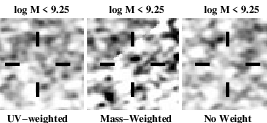
For stacks of sources with stellar masses less than , we do not find a detection in the IR continuum. In an effort to provide a dramatic illustration of this, we include in Figure 10 three different stacks of all 1253 –10 sources with stellar mass estimates 109.25 over our ASPECS footprint. Our first stack weights sources by their flux, our second stack weights sources by their estimated stellar mass, and our third stack weights sources equally (left, center, and right panels, respectively). None of the stacks show a significant detection, and in our unweighted stack, the mean continuum flux density is 0.10.40.4Jy beam-1. Even weighting sources in the stack by the measured -continuum slope fails to result in a significant detection. This demonstrates, rather dramatically, that faint, UV-selected galaxies show essentially no dust continuum emission (see also Carvajal et al. 2020). Converting this flux density constraint to a star formation rate for a galaxy at , we derive a SFR of 0.00.1 yr-1.
III.3.2 Infrared Excess versus
Stacked results of –3.5 and –10 sources over our ASPECS footprint are presented as a function of -continuum slope in Figure 11 with the large solid circles and upper limits. Five different bins in are utilized to better map out the trend with -continuum slope .
Separate stack results are presented for sources with stellar masses (large red circles and downward arrows, respectively) and (large green circles and downward arrows, respectively) to evaluate whether higher-mass galaxies show a different IRX- relationship from lower-mass galaxies. This treatment also ensures that results in the redder, high-mass bins are not impacted by the inclusion of bluer, lower-mass sources (but where the measured -continuum slopes are much redder than the actual slopes due to the impact of noise). Figure 12 presents our stack results for star-forming galaxies which are individually undetected (4). Our IRX- stack results are presented in Table 4 in the main text and Table 11 in Appendix C.
For our highest-mass –3.5 samples, our stack results lie closest to the Reddy (Calzetti-like) IRX- relations. As in our earlier analysis of the ASPECS pilot data, we formalize this analysis by finding those parameters which best match the stacked IRX results vs. and then computing 68% confidence intervals on the derived parameters. Here we derive constraints on both and as
| (9) |
instead of just deriving constraints on as in our previous analysis.
Our maximum-likelihood derived values for and are 1.81 and and presented in Table 5. The we derive is similar to the Calzetti or Reddy value, i.e., 1.97 or 1.84. Meanwhile, the we derive is not only redder than the implicit in the Meurer et al. (1999) formulation, but also redder than what might be expected for dust-free galaxies with a constant star formation rate for 100-500 Myr (e.g., as in Reddy et al. 2018). Both the and we derive are consistent with the consensus low-redshift values for these quantities (e.g., Eq 4). If we instead take as has been conventional (following Meurer et al. 1999), the we recover is 1.48. In our pilot study, our best-fit determination for is 1.26 when taking equal to . For a , we recover equal to 1.42.
| Stellar | # of | ||
|---|---|---|---|
| Mass () | sources | IRXaaBoth the bootstrap and formal uncertainties are quoted on the result (presented first and second, respectively). | |
| –3.5 | |||
| All | 5 | 51.341.29 | |
| - | All | 6 | 26.990.64 |
| - | All | 11 | 16.730.51 |
| - | All | 33 | 2.230.23 |
| - | All | 123 | 0.900.38 |
| All | 467 | 0.720.66 | |
| –10 | |||
| All | 1 | 19.081.02 | |
| - | All | 6 | 0.221.11 |
| - | All | 31 | 4.120.49 |
| - | All | 69 | 0.410.61 |
| All | 594 | 0.720.59 | |
| –10 | |||
| All | 1253 | 0.500.31 | |
| –3.5 | |||
| 4 | 0.020.21 | ||
| 16 | 6.540.28 | ||
| 14 | 10.270.30 | ||
| 4 | 174.573.32 | ||
| 369 | 0.830.43 | ||
| 204 | 0.840.36 | ||
| 34 | 5.571.13 | ||
| –10 | |||
| 537 | 0.240.37 | ||
| 125 | 0.650.56 | ||
| 32 | 7.670.96 | ||
For lower-mass (109.5 ) –3.5 galaxies found over ASPECS, significant ALMA continuum flux is found in two of the three bins we consider. Fixing to be the same as for the higher-mass galaxies, we find a best-fit value for of 1.12. This is most consistent with an SMC-like dust curve, but is nevertheless consistent with our constraints on the value in the higher mass 109.5 bin.

| Sample | Mass Range | ||
|---|---|---|---|
| Current Determinations | |||
| –3.5 | 1.81 | ||
| –3.5 | 1.12 | (fixed) | |
| –3.5 | 1.48 | (fixed) | |
| –3.5 | 1.42 | (fixed) | |
| Canonical IRX- Relations | |||
| Consensus: aaTaking the median of the IRX- relations derived by Overzier et al. (2011), Takeuchi et al. (2012), and Casey et al. (2014). See Appendix B. | 1.86 | 1.87 | |
| Reddy et al. 2015: | 1.84 | 2.43 | |
| Overzier et al. 2011: | 1.96 | 1.96 | |
| Takeuchi et al. 2012: | 1.58 | 1.94 | |
| Casey et al. 2014: | 2.04 | 1.64 | |
| Meurer et al. 1999: | 1.99 | 2.23 | |
| Dust Laws | |||
| Calzetti | 1.97 | — | |
| SMC | 1.10 | — | |
We now look at the constraints we can set on the IRX- relationship at –10. We focus on sources with the highest stellar masses, i.e., 109.25 to minimize the impact of intrisically blue, lower-mass sources scattering to redder colors (see §3.1.1 from Bouwens et al. 2016). Our –10 stack results for sources shows prominent detections in the reddest two bins, one at and 1.6. Those two detections imply very different IRX- relationships. Fixing the value of to be and fitting to the two bluest bins plus the bin, we derive a value of 2.27. By contrast, if we fit to the two bluest bins plus the bin, we derive a value of 0.63. Given how different the two relations are and the fact that there are only two significant detections at we can use from ASPECS, perhaps it is best for us simply to quote our –10 results as the range spanned by these two relations. As this range includes both Reddy/Calzetti-like and SMC-like dust relations, the ASPECS data provide us with very little information on how the IRX- relation evolves.
III.3.3 Summary of Stack Results
Our convenient summary of our main stack results as a function of stellar mass, redshift, and is provided in Table 4. For a more detailed breakdown of these stack results and comparison with expectations, we refer the interested reader to Appendix C.
III.4. Infrared Excess as a bivariate function of stellar mass and
III.4.1 Correlation with Stellar Mass and -continuum Slope
Having looked at the correlation of the infrared excess with the stellar mass and -continuum slope , it is interesting to try to link these relations based on the empirical correlation of these two quantities with each other based on the large samples that now exist based on various legacy data sets. Given the significant correlation between the dust content and metallicity of galaxies and their stellar mass (e.g., Reddy et al. 2010; Pannella et al. 2015), one would expect a strong correlation between the -continuum slope of galaxies and their stellar mass, as in fact is observed (e.g., McLure et al. 2018; Carvajal et al. 2020).
For this exercise, we take all the –2.5 sources identified over the five CANDELS fields by 3DHST team (Skelton et al. 2014) and compare their -continuum slopes with their stellar masses derived by Prospector (Leja et al. 2017, 2019). The results are presented in Figure 7, and it is clear that for sources with stellar masses to the -continuum slopes of galaxies generally lie in the range to . For sources with stellar masses 109 , the -continuum slopes show a strong correlation with stellar mass to .
Using the correlations we derive between the infrared excess and the stellar mass (§3.3.1),
| (10) |
and between the infrared excess and the -continuum slope (§3.3.2)
| (11) |
This results in
| (12) |
Fixing and taking the best-fit value we find for (i.e., 1.42), we look for the optimal values of and to capture the observed relationship between stellar mass and -continuum slope shown in Figure 7. In deriving this relationship, we segregate sources into those above and below the vs. relation, determine the number of such sources in six distinct regions along the relation, compute the square of the difference in the number of sources on each side for each of the six regions, and then minimize the square of the differences. The best-fit values of and are 109.07 and 0.92, respectively. This best-fit relation is included in Figure 7 with the blue line. For comparison, Figure 7 also shows the vs. stellar mass relationship derived by McLure et al. (2018). Encouragingly enough, the best-fit value for and are consistent (at ) with the values we derive from our IRX-stellar mass analysis, i.e., and 0.97, respectively, demonstrating that the IRX- and IRX-stellar mass relations we derive are essentially equivalent.

III.4.2 Infrared Excess of a Function of Stellar Mass and -continuum Slope
Having quantified the approximate relationship between the stellar mass and -continuum slope of galaxies at -2.5, we now move on to try to express the infrared excess as a bivariate function of the -continuum slope and the stellar mass .
One reason for pursuing such a parameterization would be to take advantage of the greater information content present in both the measured -continuum slope and the inferred stellar mass of a galaxy. While the two parameters are clearly correlated (e.g., §III.4.1), the two parameters do provide us with independent information on sources and therefore theoretically should be able to improve our estimates of the infrared excess.
We use the following functional form:
| (13) |
where is as follows and gives the expected stellar mass for a given -continuum slope (as derived in the previous subsection):
| (14) |
The expression we adopt for is the standard form for the IRX- relation, but then allows for a dependence on whether a source is more or less massive than one would expect for a given -continuum slope .
Sources from ASPECS were divided in stellar mass and in the same way as the previous sections, stacked using the same weighting scheme as described in §3.3, and then an average infrared excess derived for each stellar mass- bin. The derived infrared excesses vs. and stellar mass were then fit using the expression given in Eq. 13. The best-fit values we recovered for and were 1.480.10 and 0.670.06. Encouragingly enough, the best-fit value for is very similar to what we found expressing the infrared excess as a function of the -continuum slope alone. We do find a minor additional dependence on whether the inferred stellar mass is greater or less than given by the general correlation between stellar mass and , but the dependence is not particularly strong. The blue lines in Figure 13 presents the suggested regions in / parameter space with infrared excesses of 4, 20, and 100, shown relative to the detected and undetected sources from ASPECS.
Álvarez-Márquez et al. (2019) had previously attempted to quantify the infrared excess as a function of both the UV-continuum slope and stellar mass, as . While the functional form Álvarez-Márquez et al. (2019) utilize is different from what we consider, it is interesting to try to compute the logarithmic dependence of IRX on and to investigate how similar the results are. For simplicity, we compute the dependence at a and of 1010.5 . For the function we derive, we compute a of 0.18 and a of 0.67 vs. 0.510.06 and 0.370.08 found by Álvarez-Márquez et al. (2019). These relations are in reasonably good agreement, which is encouraging given the differences in approach (the Álvarez-Márquez et al. 2019 are based on deep Herschel stacks).
| Predicted [Jy] | Measured | ||||||||
|---|---|---|---|---|---|---|---|---|---|
| ID | aaFrom Eq. B4 (Appendix B), which is the Meurer et al. (1999) IRX- relationship. | bbFrom Eq. 4, which is the consensus low-redshift IRX- relation derived here in Appendix B from literature results. | ccEq. 6, which gives an SMC-like IRX- relation | ddFrom Eq. 3, which is the consensus IRX-stellar mass relation presented in our previous study Bouwens et al. (2016) | eeFrom Eq. 9, which is the IRX- relation we derived for 109.5 , –3.5 galaxies (§III.3.2). | ffFrom Eq. 8, which is the IRX-stellar mass relation we derived for –3.5 galaxies (§III.3.1). | ,M)ggFrom Eq. 13, which is the IRX(, M) relation we derived (§III.4.2). | hhGeometric mean of our derived –3.5 IRX- relation and our IRX-stellar mass relationship . | [Jy] |
| XDFU-2435246390 | 60 | 24 | 7 | 63 | 23 | 58 | 50 | 36 | 107146 |
| XDFU-2385446340 | 184 | 66 | 31 | 111 | 65 | 110 | 126 | 85 | 75210 |
| XDFU-2397246112 | 380 | 151 | 45 | 642 | 143 | 587 | 436 | 290 | 46114 |
| XDFU-2369747272 | 1572 | 534 | 56 | 43 | 469 | 40 | 82 | 137 | 4329 |
| XDFU-2400547554 | 1434 | 571 | 177 | 1492 | 541 | 1391 | 1206 | 868 | 34218 |
| XDFU-2410746315 | 41 | 16 | 6 | 3 | 15 | 3 | 6 | 7 | 31611 |
| XDFU-2433446471 | 173 | 64 | 11 | 44 | 58 | 40 | 47 | 48 | 28921 |
| XDFU-2350746475 | 710 | 264 | 47 | 148 | 240 | 137 | 170 | 182 | 23311 |
| XDFU-2416846554 | 294 | 109 | 19 | 21 | 99 | 20 | 34 | 44 | 18510 |
| XDFB-2380246263 | 262940 | 73791 | 2555 | 514 | 60164 | 480 | 1716 | 5373 | 16310 |
| XDFB-2355547038 | 124 | 49 | 18 | 11 | 47 | 12 | 22 | 23 | 1559 |
| XDFU-2387248103 | 203 | 81 | 26 | 10 | 77 | 10 | 22 | 28 | 13424 |
| XDFU-2373546453 | 655 | 261 | 91 | 474 | 250 | 452 | 451 | 336 | 10710 |
| XDFU4596 | 459 | 183 | 61 | 259 | 174 | 248 | 263 | 208 | 979 |
| XDFU-2361746276 | 552 | 218 | 60 | 225 | 205 | 213 | 238 | 209 | 8512 |
| XDFU9838 | 253 | 100 | 28 | 56 | 94 | 54 | 73 | 71 | 6515 |
| XDFU-2359847256 | 145 | 56 | 23 | 123 | 54 | 119 | 119 | 80 | 5810 |
| XDFU-2370746171 | 244 | 85 | 40 | 67 | 84 | 69 | 100 | 76 | 4711 |
| PerformanceiiSee §III.5 for a discussion | |||||||||
| 25%/75% Quartiles | [23.2,1.7] | [8.0,0.8] | [2.0,4.0] | [4.8,1.1] | [7.2,0.8] | [4.8,1.0] | [5.5,0.9] | [3.8,1.3] | |
| 25%/75% Quartiles | [1.1,0.4] | [1.1,0.6] | [1.1,1.4] | [1.1,0.7] | [1.1,0.7] | [1.1,0.7] | [1.1,0.3] | [1.1,0.6] | |
| jjOnly for those 25 sources where | |||||||||
| Mean / Std. Dev. | 0.420.81 | 0.010.80 | 0.540.70 | 0.290.69 | 0.030.79 | 0.300.68 | 0.140.65 | 0.170.67 | |
| Median | 0.59 | 0.19 | 0.37 | 0.12 | 0.16 | 0.12 | 0.05 | 0.02 | |
Given the strong correlation between both parameters, where (see §III.4.1), it is also interesting to reformulate the Álvarez-Márquez et al. (2019) IRX relation to be just a single function of . We find . If we make the same change to our bivariate relation, we find . As with the previous comparison, the two dependencies are similar, which is encouraging given differences in the two approaches.
III.5. Predictive Power of Different Estimators for IRX
Before concluding this section, it is useful to summarize the predicted 1.2mm flux densities expected for different galaxies over the ASPECS footprint and compare those predictions with the observations. A compilation of the results are presented in Table 6 and include the predicted flux densities using (1) the Meurer et al. (1999) IRX- relation (Eq. B4: Appendix B), (2) the consensus low-redshift IRX- relation (Eq. 4) derived here in Appendix B from literature results, (3) an SMC-like IRX- relation (Eq. 6), (4) the consensus IRX-stellar mass relation (Eq. 3) presented in our previous study Bouwens et al. (2016), (5) our derived IRX- relation for 109.5 , –3.5 galaxies (Eq. 9: §III.3.2), (6) our derived IRX-stellar mass relation for –3.5 galaxies (Eq. 8: §III.3.1), and (7) our derived IRX(, M) relation (Eq. 13: §III.4.2). As one final predictor, we include a comparison against the flux density predicted taking the geometric mean of our derived –3.5 IRX- relation and our IRX-stellar mass relationship, i.e., , and using Eqs. 9 and 8 while taking , , , and to be 1.81, , , and 0.97, respectively. This should provide for an alternate way of using both the -continuum slopes and stellar masses in estimating the infrared excess.
The observed fluxes are also explicitly compared against these many estimators in Figure 14. A quantification of the mean, median, and scatter in the logarithmic ratio of the predicted and measured 1.2mm flux densities is presented in Table 6, and it is clear there is substantial scatter between the observed and predicted flux densities. The scatter ranges from 0.65 to 0.81 dex, with the smallest dispersion found for the and estimators, with only slight increases in the dispersion for the other relations. The and estimators also provide the best predictions of the observed flux densities in the median.
As a separate means of evaluating the estimators, we compare the predicted 1.2mm flux densities from these estimators with the measured flux densities using both the detected sources in Table 6 and sources expected to be detected at 2 averaging the IRX- and IRX-stellar mass relations derived here (Eqs 9 and 8), i.e., 70 sources in total. For each of these sources, we computed the difference between the measured and predicted flux for each source, i.e., and , divided the result by the measurement error , and then determined the average as well as the upper and lower quartiles. For almost every estimator, the difference between the upper and lower quartiles is larger than the measurement error by 5.
For each of the estimators, we also computed the differences between the measured and predicted flux densities for the same sources as the previous exercise, divided the result by the root mean square of the predicted flux densities and flux measurement uncertainties, and finally computed the upper and lower quartiles. This should give an approximate relative uncertainty on the flux density predictions. All of our estimators perform comparably well, with only modest differences between them.
In summary, as with previous work (e.g., Meurer et al. 1999; Reddy et al. 2006), estimators of the infrared excess tend to be accurate in predicting the obscured star formation rates or IR luminosities for the average source and tend to show at least 0.65 dex scatter for individual sources. Of those we consider, the different estimators for the infrared excess all perform comparably, with marginally better performance for the estimators that consider both mass and , i.e., and , while the estimator performed the least well.
IV. Discussion
IV.1. Previous Reported Continuum Detections
It is interesting to compare the present set of ALMA continuum detections to those that were previously reported over the HUDF by Aravena et al. (2016), Bouwens et al. (2016), and Dunlop et al. (2017). The reported detections and tentative detections by Aravena et al. (2016) and Bouwens et al. (2016) made use of the 1 arcmin2 pilot for ASPECS, while the Dunlop et al. (2017) results were based on the 1.3mm ALMA continuum observations they obtained over a 4.5 arcmin2 region within the HUDF/XDF.


Using the 1 arcmin2 pilot observations for ASPECS, Aravena et al. (2016) and Bouwens et al. (2016) detected 5 galaxies and reported tentative detections for 3 more galaxies. Our new observations confirm all of our previously claimed detections at 4, making it clear that those detections were real. In addition, one of the tentatively detected sources from our pilot program, i.e., XDFU-2370746171, shows a 4 detection (4011Jy beam-1) in the new data, confirming that the reported tentative detection (3414Jy beam-1) from our pilot was real.
The measured flux densities for the two other tentative detections from our pilot, i.e., XDFU-2365446123 and XDFU-2384246384, are 2717 Jy beam-1 and 810 Jy/beam vs. our measurements of 3816Jy/beam and 3614Jy/beam, respectively, in the pilot for these sources. Combining the measurements, the flux is 712Jy beam-1 for XDFU-2365446123 and 178Jy for XDFU-2384246384. While the new observations do not support the reality of either source, XDFU-2384246384 still shows a tentative 2.1 detection in the continuum in the combined data set and thus may be real.
In the Dunlop et al. (2017) search, 16 dust-continuum (3.5) detections are identified, 11 of which have an estimated redshift in excess of 1.5 and lie within the ASPECS footprint. 8 of these 11 sources are clearly confirmed with our ASPECS ALMA observations. For the 3 reported continuum detections from the Dunlop et al. (2017) which are not unambiguously confirmed by our ASPECS observations, we measure Jy (UDF9), Jy (UDF12), and Jy (UDF15).
IV.2. Comparison with Previous Determinations of the Infrared Excess
It is interesting to compare the IRX-stellar mass and IRX- relations we derive with the many previous determinations in the literature. We focus on determinations at –3.5 since this is where our results are the most significant and where most of previous results have been obtained. In Figure 15, we compare the IRX-stellar mass relationship we find at –3.5 with what we obtained in our pilot study (Bouwens et al. 2016) and many other determinations in the literature (McLure et al. 2018; Reddy et al. 2018; Pannella et al. 2015; Fudamoto et al. 2017, 2020a; Bourne et al. 2017; Álvarez-Márquez et al. 2016, 2019; Heinis et al. 2014; Koprowski et al. 2018).
Overall, our new IRX-stellar mass results appear to be in agreement with previous results as presented e.g. by Heinis et al. (2014), Pannella et al. (2015), Bourne et al. (2017), and McLure et al. (2018), or even as given by the consensus relation derived in our pilot study (shown with the grey line). Our best-fit IRX-stellar mass correlation is 0.2-0.3 dex higher at 1010 than found in our earlier study (Bouwens et al. 2016) but consistent within the quoted uncertainties. Thanks to the larger number of dust-continuum detected sources in the current ASPECS study vs. our pilot study (18 vs. 3 detections), we are able to significantly improve our quantification of the IRX-stellar mass relation relative to our previous study.
The slope recovered for our new IRX-stellar mass relation, i.e., 0.97, is very close to one. We had previous adopted a value of unity in Bouwens et al. (2016) for the consensus relation (Eq. 3) based on the IRX-stellar mass results of Reddy et al. (2010), Whitaker et al. (2014), and Álvarez-Márquez et al. (2016). The IRX - stellar mass relation derived by McLure et al. (2018) using the shallower ALMA observations over the HUDF (Dunlop et al. 2017) also find a slope (0.850.05), very close to what we find here. At one other extreme, Fudamoto et al. (2020a) recover a much steeper slope (1.640.10) for the IRX-stellar mass relation, similar to what we derive using Prospector for our stellar mass estimates (Appendix D). Meanwhile, earlier results obtained from an analysis of Herschel data by Pannella et al. (2015) find a much shallower IRX-stellar mass relation, with a slope of 0.64, clearly shallower than what we find here (see also results by Álvarez-Márquez et al. 2019). Given the current strong constraints on the obscured SFR at low masses (109.25 ) and the challenge that source confusion presents for the lowest mass sources with Herschel, it seems likely that the slope of the infrared excess is approximately unity or steeper, as essentially all analyses relying on ALMA data have found.

| Dust Correction | ||
|---|---|---|
| Sample | (0.05 )aaThe specified limits 0.05 and 0.03 correspond to faint-end limits of and , respectively, which is the limiting luminosity to which and galaxies can be found in current probes (Schenker et al. 2013; McLure et al. 2013; Ellis et al. 2013; Oesch et al. 2013; Bouwens et al. 2015). | (0.03 )aaThe specified limits 0.05 and 0.03 correspond to faint-end limits of and , respectively, which is the limiting luminosity to which and galaxies can be found in current probes (Schenker et al. 2013; McLure et al. 2013; Ellis et al. 2013; Oesch et al. 2013; Bouwens et al. 2015). |
| 0.37**For uniquely the sample, we make use of the finding by e.g. Reddy & Steidel (2004) and Reddy et al. (2010) that the average infrared excess for galaxies brighter than 25.5 mag at is a factor of 5. | 0.34**For uniquely the sample, we make use of the finding by e.g. Reddy & Steidel (2004) and Reddy et al. (2010) that the average infrared excess for galaxies brighter than 25.5 mag at is a factor of 5. | |
| 0.33 | 0.31 | |
| 0.30 | 0.27 | |
| 0.20 | 0.17 | |
| 0.09 | 0.07 | |
| 0.07 | 0.06 | |

The IRX-stellar mass results we obtain at –10 can be compared with results obtained using a small sample of bright -6 galaxies from Capak et al. (2015) and Willott et al. (2015) and assuming the dust temperature evolution given in Eq. 1. Also included in this comparison are the new ALPINE results from Fudamoto et al. (2020b), both as quoted in the original study (solid colored points) and adopting the fiducial dust temperature evolution adopted here (Eq 1). This comparison is presented in Figure 16. Our own results appear to be most consistent with the consensus IRX-M∗ relationship we had derived in our pilot study (Bouwens et al. 2016) and as now derived here as –3.5. While this suggests that the IRX-stellar mass relation may extend to –6 with little or no evolution, the ASPECS field only contains a few bright, massive sources to probe this well. Additionally, this inference depends critically on the dust temperature being relatively high, i.e., 50 K, at –6. If the temperature is instead 41 K as Fudamoto et al. (2020b) adopt in their analysis, clearly the IRX-stellar mass relation at is lower than what is found at –3.5.
In Figure 17, we compare the IRX- relationship we derive for higher-mass, –3.5 galaxies with the results obtained in our pilot study (Bouwens et al. 2016) as well as a wide variety of different determinations in the literature (McLure et al. 2018; Reddy et al. 2018; Álvarez-Márquez et al. 2016, 2019; Fudamoto et al. 2017, 2020a; Heinis et al. 2013; Bourne et al. 2017; Koprowski et al. 2018). Similar to what we found for the IRX-stellar mass relation, the larger number of dust-continuum detections found here (vs. from the smaller-area ASPECS pilot) results in our recovering a steeper IRX- relation than in our pilot, i.e., 1.48 vs. when fixing . The only apparently significant difference occurs for our determination at 1.3 where the limit from our pilot program was 1.310.72 (at ) and where our new measurement is 6.540.28 (at ). This difference results both from the larger number of dust detected sources in the larger area probed by ASPECS (vs. our PILOT) and from our changing the binning scheme to exploit the larger number of sources to improve our leverage for constraining the IRX- relation.
Relative to various determinations from the literature, the most significant differences occur for the bluest values of , i.e., , where our own determination of the infrared excess is some 0.2-1.0 dex lower than the determinations of Reddy et al. (2018), Fudamoto et al. (2017), Bourne et al. (2017), and McLure et al. (2018). It seems likely that the differences here are due to the presence of blue, IR-luminous sources in many previous selections. While blue, IR-luminous galaxies are known to exist (e.g., Reddy et al. 2006; Casey et al. 2014), especially at high IR luminosities (1012 ) where there is less connection between the and morphologies in galaxies, these sources are not sufficiently common to be well sampled by the 2.5104 comoving Mpc3 volume probed by ASPECS at –3.5.


Otherwise, our IRX- results are broadly in agreement with the results of Reddy et al. (2018), Álvarez-Márquez et al. (2016), and Heinis et al. (2013). For redder values of , our IRX- results are lower than the results of McLure et al. (2018), Fudamoto et al. (2017), Bourne et al. (2017), and Fudamoto et al. (2020a) by 0.4 dex. We expect that some fraction of these differences, i.e., 0.3 dex, could result from different calibrations to derive the IR luminosities and obscured SFRs from the measured ALMA fluxes (e.g., Murphy et al. 2011 vs. Whitaker et al. 2017).
IV.3. Dust Corrections for Samples
The purpose of this section is to take advantage of the results of our analyses from the previous sections to derive dust corrections that we can apply to the general star-forming galaxy population at .
We will focus on deriving these corrections as a function of the luminosity of galaxies and derive a distribution of dust corrections that make up each luminosity bin. To ensure a significant sampling of each luminosity bin, we leverage the large selections of star-forming galaxies Bouwens et al. (2015) identified at , 5, 6, 7, 8, and 10 over the CANDELS GOODS-North and GOODS-South.
Each of the sources over the CANDELS GOODS-North and GOODS-South fields has sensitive HST optical/ACS and WFC3/IR photometry available to derive -continuum slopes for each source in these samples. Another valuable aspect of sources in these fields is the deep Spitzer/IRAC observations that exist from the 200-hour GREATS program (Labbé 2014; Stefanon et al. 2020) to provide rest-optical photometry for –8 galaxies and thus to estimate stellar masses. HST and Spitzer/IRAC photometry is performed on sources in these fields in a similar way to described in §2.2, and -continuum slopes and stellar masses are estimated using the FAST stellar population fitting code as described in §2.5.
In deriving dust corrections for each bin in luminosity, we make use of the stellar masses and -continuum slopes derived for our large CANDELS samples and utilize the new relation Eq. 13 we derived in §3.4.2 for the infrared excess IRX expressed as a function of both and stellar mass . To ensure that our extinction estimates are not overly impacted by noise in the photometry scattering lower-mass sources to red measurements, we force the infrared excesses of sources with stellar masses less than 109 to be zero, consistent with our derived observational constraints.
For convenience, we present the dust corrections we have derived here in Table 7. If the dust temperatures of galaxies are in fact closer to 35 K than given by our fiducial dust temperature model, the dust correction we compute would be approximately half as large. As in Bouwens et al. (2016), we assume that the average dust correction for UV bright (25.5 mag) galaxies at is 5 following the findings of Reddy & Steidel (2004).
| Lyman | Dust | SFR density | ||||
|---|---|---|---|---|---|---|
| Break | (erg s-1 | Correction | ( Mpc-3 yr-1) | |||
| Sample | Hz-1 Mpc-3)aaIntegrated down to 0.03 . Based upon LF parameters in Table 6 of Bouwens et al. (2015). The SFR density estimates assume Myr constant SFR and a Chabrier IMF (Madau & Dickinson 2014). Conversion to a Salpeter (1955) IMF would result in a factor of 1.6 (0.2 dex) increase in the SFR density estimates given here. | (dex)bbThe contribution indicated here is our fiducial estimate from far-IR bright, ULIRG-like ( ) galaxies (see Fig. 18). The SFR density contribution for the far-IR bright population tends to be either missed completely due to these sources not being selected in Lyman-break galaxy probes (e.g., Simpson et al. 2014) or significantly underestimated due to the IR luminosities underestimated based on their properties (e.g., Reddy & Steidel 2009). | Uncorrected | Corrected | Incl. ULIRGbbThe contribution indicated here is our fiducial estimate from far-IR bright, ULIRG-like ( ) galaxies (see Fig. 18). The SFR density contribution for the far-IR bright population tends to be either missed completely due to these sources not being selected in Lyman-break galaxy probes (e.g., Simpson et al. 2014) or significantly underestimated due to the IR luminosities underestimated based on their properties (e.g., Reddy & Steidel 2009). | |
| U | 3.0 | 26.550.06 | 0.44 | 1.600.03 | 1.260.09 | 1.160.09 |
| B | 3.8 | 26.520.06 | 0.39 | 1.630.06 | 1.320.06 | 1.240.06 |
| V | 4.9 | 26.300.06 | 0.32 | 1.850.06 | 1.580.06 | 1.530.06 |
| i | 5.9 | 26.100.06 | 0.20 | 2.050.06 | 1.880.06 | 1.850.06 |
| z | 6.8 | 25.980.06 | 0.07 | 2.170.06 | 2.100.06 | 2.100.06 |
| Y | 7.9 | 25.670.06 | 0.06 | 2.480.06 | 2.420.06 | 2.420.06 |
| J | 10.4 | 24.62 | 0.00 | |||
IV.4. Star Formation Rate Densities at
As in the analysis for our pilot study, we apply the dust corrections we derive in the previous section to the luminosity densities integrating the LF of Bouwens et al. (2015) to 0.05 (17.7 mag) and to 0.03 (17.0 mag). As in previous work, the luminosity densities are converted into SFR densities using the Madau & Dickinson (2014) conversion factor (see also Madau et al. 1998 and Kennicutt 1998) modified to assume a Chabrier (2003) IMF:
| (15) |
This relationship assumes a constant SFR for 100 million years. We also apply these dust corrections to the Reddy & Steidel (2009) and McLure et al. (2013) LF results. Our quantitative results for the corrected and uncorrected SFR densities at –10 are presented in Table 8.
In computing the SFR density, we must account not only for the impact of dust extinction on the luminosities themselves but also for the more massive, far-infrared bright sources where standard dust corrections are not effective or which are sufficiently faint in the to be entirely missed in standard LBG searches (e.g., Reddy et al. 2006, 2008; Swinbank et al. 2014; Casey et al. 2018; Williams et al. 2019; Dudzevičiūtė et al. 2020). Such sources are known to contribute a substantial fraction of the SFR density at –3 (Hughes et al. 1998; Blain et al. 1999; Lilly et al. 1999; Chapman et al. 2005; Barger et al. 2012; Karim et al. 2011; Magnelli et al. 2013; Madau & Dickinson 2014; Swinbank et al. 2014; Wang et al. 2019; Dudzevičiūtė et al. 2020). Perhaps the best way to account for these galaxies (proposed earlier by Reddy et al. 2008) is to simply include them based on dedicated searches for these sources in the IR.
We consider the results of Magnelli et al. (2013) at –2 (which build on the results of Caputi et al. 2007 and Magnelli et al. 2009, 2011), the Franco et al. (2020a) results at –5 from a 69 arcmin2 survey area, the Yamaguchi et al. (2019) results at –5 from the 26 arcmin2 ASAGAO survey area, and the Williams et al. (2019) serendipitious discovery of a probable dusty SF source at . We compute the SFR density contribution from ULIRG-type galaxies at from ASPECS volume by converting the measured ALMA fluxes from detected sources in their survey area to SFRs assuming 100% of the energy comes from star formation, binning the contributions by the derived redshifts for the sources, and then dividing by the cosmic volume within a 4.2 arcmin2 survey area, finding 0.0360.022 yr-1. We use a similar approach derive the SFR density contribution from ULIRGs at –5 from the 69-arcmin2 Franco et al. (2020a) probe, but given the limited depth of the Franco et al. (2020a) probe, we treat this derived contribution as a lower limit. The Franco et al. (2020a) probe builds on the earlier Franco et al. (2018) study using deeper search results presented in Franco et al. (2020b).
Additionally, we consider the integrated SFR density derived from MAGPHYS fits to the 1 deg2 AS2UDS sample by Dudzevičiūtė et al. (2020), who corrected for incompleteness using the number counts from Geach et al. (2017) and extrapolated from the observed 870m flux limit of 3.6 mJy for the SCUBA-2 survey to 1 mJy using the slope of the number counts from Hatsukade et al. (2018). See §5.4 and Figure 15 from Dudzevičiūtė et al. (2020). The uncertainties on the values were calculated by resampling the SFR and redshift probability distributions of each source. The approximate survey volume for the AS2UDS results is approximately 7107 Mpc3 and so likely to be much more representative than smaller volume studies.
Finally, we also estimate the SFR density from ULIRG-type sources by assuming the star-forming main sequence results of Speagle et al. (2014) apply to the wide-area –3 mass functions of Ilbert et al. (2013) and –6 mass functions of Davidzon et al. (2017). Encouragingly enough, the estimated SFR contribution provided by ULIRG-type galaxies using the observed mass functions appears to plausibly consistent with that derived from constraints available from direct searches for ULIRG-type sources at –4 and 0.2 dex higher at –6.

A summary of the inferred SFR density for all the aforementioned ULIRG probes is presented in Figure 18. As our fiducial estimate of the obscured SFR density from ULIRGs, we adopt the Magnelli et al. (2013) constraints at , our mass function derived estimate at , the AS2UDS estimates (Dudzevičiūtė et al. 2020) at –6, and the Wang et al. (2019) at . We have indicated fiducial obscured SFR densities in Figure 18 with the hatched red area. This fiducial model is most consistent with the dust poor model from Casey et al. (2018).
We combine these SFR densities with those we derived by correcting the LFs at –10 to present our best estimates for the SFR density at –10 in Table 8 and Figure 19, together with a few previous estimates (Schiminovich et al. 2005; Reddy & Steidel 2009; McLure et al. 2013) in Figure 19. It is interesting to compare the contribution that unobscured and obscured star formation makes to the total SFR density of the universe. Figure 20 shows such a breakdown of the SFR density. The obscured SFR density shown at is from the Magnelli et al. (2009, 2011, 2013), while at -3, the obscured SFR density shown is the sum of the SFR density from AS2UDS (Dudzevičiūtė et al. 2020) and from Reddy & Steidel (2009). The contribution to the SFR density from ULIRGs is presented for context. From the presented breakdown, we can see that star formation is mostly unobscured at , mostly obscured at , and marks the approximate transition redshift between the two regimes. Previously, Bouwens et al. (2009), Bouwens et al. (2016), and Dunlop et al. (2017) found that the approximate transition point between the two regimes was .
IV.5. Star Formation Rate Density in the ASPECS Volume
Finally, before closing the discussion we provide in this paper on the SFR density, it is interesting to try to estimate the SFR density within the ASPECS HUDF/XDF volume itself. Given the limited volume probed by ASPECS and the impact of large scale structure, this is an interesting issue to examine to help determine the extent to which conclusions drawn from the HUDF volume are applicable to much larger cosmic (106 comoving Mpc3) volumes of the universe (where the impact of large-scale structure is less).
To estimate the approximate SFR density within the ASPECS volume, we rederive the LF at , , , , , , , and but only using sources in the ASPECS/HUDF/XDF volume. For simplicity, in deriving this LF, we fix the faint-end slope and characteristic luminosity to that derived from Bouwens et al. (2015) and Bouwens et al. (2020, in prep) at these same redshifts and fit for the normalization . The relative normalization we derive for the LFs over the ASPECS areas relative to the cosmic average, i.e., is 1.17, 0.85, 0.68, 0.74, 1.10, 0.95, 0.98, 1.29, and 0.50 at , , , , , , , , and , respectively. The rms logarithmic scatter in these normalizations are 0.12 dex, i.e., fluctuations of 32% (0.12 dex) in the volume density of galaxies in a given redshift interval of the HUDF relative to the cosmic average. 32% is fairly similar to the expected variations one would expect for sources with a volume density of 110-3 Mpc-3 inside a 2 arcmin 2 arcmin volume. Figure 21 illustrates how the SFR density we infer from the HUDF might compare with the cosmic average, if we assume that we can apply the LF normalization factors just derived to the SFR density as a whole.
To assess the impact of large scale structure on the present results and other results from ASPECS, it is relevant to compare the observed 0.12-dex scatter with that expected from the relative small number of dust detected and CO-detected sources over ASPECS. In cases where the number of sources per unit redshift is in the range 10-15, i.e., similar to the number of dust detected and CO detected sources in ASPECS (e.g., González-López et al. 2020; Boogaard et al. 2019), the scatter expected from small number statistics will be comparable to that seen in terms of large-scale structure. This suggests that any conclusions drawn from the HUDF ASPECS volume should be applicable to much larger cosmic (106 comoving Mpc3) volumes, with a relatively limited impact from large-scale structure.
V. Summary
Here we make use of sensitive observations we have obtained from the ALMA large program ASPECS of far-IR continuum light for a large sample of –10 galaxies located over the Hubble Ultra Deep Field (HUDF). ASPECS probes with great sensitivity (9.3Jy beam-1: ) the 1.2 mm far-IR continuum of galaxies and extends over a 4.2 arcmin2 region using 90 hours of band-6 observations in total.
With these observations, we probe dust-enshrouded star formation to 7-28 yr-1 () from 1362 robust –10, -selected galaxies located over the ASPECS footprint. These –10 sources were either drawn from the literature (Bouwens et al. 2015) or selected specifically for this study by applying standard color selection or photometric redshift criteria to the deep WFC3/UVIS observations over the HUDF from the UVUDF program (Teplitz et al. 2013; Rafelski et al. 2015).
Eighteen of the galaxies within our ASPECS footprint are detected at 4 in our 1.2-mm continuum observations. 12 of the 18 4 detections were previously identified as part of the ASPECS pilot program (Aravena et al. 2016; Bouwens et al. 2016) or the Dunlop et al. (2017) program. Six of the reported continuum detections are new discoveries from the ASPECS large program (see González-López et al. 2020; Aravena et al. 2020).
The observed number of continuum detections is in agreement with the predictions obtained by applying a consensus low-redshift IRX- relationship derived here (Appendix B) to the highest-mass –10 galaxies found over ASPECS suggests a likely sample of 28 continuum detections, while only 16 continuum detections is predicted if only sources with stellar masses in excess of are considered. This consensus IRX- relationship is constructed by combining the IRX- relations derived in Overzier et al. (2011), Takeuchi et al. (2012), and Casey et al. (2014).
In agreement with previous studies, we find that the fraction of detected galaxies in our samples increases sharply with increasing stellar mass, with the detection fraction rising from 0% at to 85% at 1010 for sources probed to a sensitivity of 20Jy beam-1. Interestingly, at low stellar masses, i.e., 109.25 , stacking all 1253 sources in our catalogs over the ASPECS footprint, we recover an average 1.2mm flux density of 0.10.4Jy beam-1, implying that the obscured star formation rate of lower-mass galaxies is essentially zero, i.e., 0.00.1 yr-1 (converting the flux density constraint to SFR at ).
The infrared excess () of galaxies in our –3.5 sample shows a strong correlation with the estimated stellar mass , with a best-fit relation . Both the recovered normalization and slope of this relation is in agreement with previous work. The infrared excess of galaxies in our –10 sample seems to show approximately the same relationship with stellar mass. Unfortunately, there are an insufficient number of high-mass star-forming galaxies within the ASPECS volume to constrain the relation.
However, we do note that, for our particular sample of galaxies, the IRX versus stellar mass relation we derive does show some dependence on which stellar population we use to estimate stellar masses. If we instead use Prospector (Leja et al. 2017) stellar population model to estimate masses for sources in our sample instead of FAST (Kriek et al. 2009), we derive a steeper IRX stellar mass relationship.
The IRX- relation we recover for higher-mass ( ) –3.5 galaxies is most consistent with a Calzetti-like IRX- relation (here represented with the Reddy et al. 2015 dust curve). The relation we derive is somewhat steeper than we previously derived (Bouwens et al. 2016), but is nevertheless consistent. Our new IRX- relation is similar to that derived by many previous teams (Reddy et al. 2018; Álvarez-Márquez et al. 2016; Heinis et al. 2013), but lower than some others (McLure et al. 2018), especially at blue ’s (i.e., ). For lower-mass –3.5 galaxies, the IRX- relation we derive is most consistent with an SMC-like relation.
Using stellar-mass and measurements for galaxies over CANDELS, we derive the following relation between and stellar mass:
| (16) |
We then use this correlation to show that our IRX- and IRX-stellar mass relations are closely connected (see also McLure et al. 2018; Carvajal et al. 2020). We then use these constraints to express the infrared excess as the following bivariate function of and stellar mass:
The best-fit values we derive for and are 1.480.10 and 0.670.06, respectively, using our ASPECS measurements.
We quantify the stacked constraints on the infrared excess in galaxies as a function of stellar mass and results and recover results at consistent with what we find at –3.5 if we assume a significant evolution in dust temperature with redshift (e.g., as found by Schreiber et al. 2018 or using our Eq. 1). If the dust temperature of –10 galaxies instead remains fixed at 35 K (e.g. Dudzevičiūtė et al. 2020), we recover infrared excesses at that are 0.4 dex lower than at –3.5.
Finally, we make use of our improved constraints on the dependence of the infrared excess on and stellar mass to provide new estimates of the dust corrections for the general star-forming galaxy population at . We determine these dust corrections as a function of luminosity and use the measured continuum slopes, stellar masses, and luminosities for large numbers of , 5, 6, 7, and 8 galaxies identified over the CANDELS GOODS-South and GOODS-North fields to compute these corrections.
We then leverage these new dust corrections and the LF determinations from Bouwens et al. (2015) to provide updated estimates of the SFR density at –10. We explicitly subdivide these SFR density estimates into the obscured and unobscured contributions and show that the SFR density transitions from being primarily unobscured to obscured at . Previously, Bouwens et al. (2009), Bouwens et al. (2016), and Dunlop et al. (2017) found that the approximate transition point between the two regimes was .
In the future, we can look forward to further significant progress in our understanding of obscured star formation at high redshift from targeting large numbers of moderate to high mass galaxies at as is being done with the ALPINE program (Le Fevre et al. 2019; Fudamoto et al. 2020b). Improvements in our constraints on the dust temperatures of galaxies from shorter and longer wavelength observations will be valuable in computing more accurate IR luminosities of individual sources. Also important will be the discovery of larger, statistical samples of IR-luminous, dusty star forming galaxies (e.g., Dudzevičiūtė et al. 2020) to achieve a more complete census of the total SFR density at . Finally, at the extreme low-luminosity end, further progress will be made in searching for obscured star formation in individual low luminosity sources through the ALMA Lensing Cluster Survey large program (2018.1.00035.L, PI: Kohno).
References
- Álvarez-Márquez et al. (2016) Álvarez-Márquez, J., Burgarella, D., Heinis, S., et al. 2016, A&A, 587, A122
- Álvarez-Márquez et al. (2019) Álvarez-Márquez, J., Burgarella, D., Buat, V., et al. 2019, A&A, 630, A153
- Aravena et al. (2016) Aravena, M., Decarli, R., Walter, F., et al. 2016, ApJ, 833, 68
- Aravena et al. (2020) Aravena, M., Boogaard, L., Gónzalez-López, J., et al. 2020, ApJ, 901, 79
- Bacon et al. (2017) Bacon, R., Conseil, S., Mary, D., et al. 2017, A&A, 608, A1
- Baker et al. (2001) Baker, A. J., Lutz, D., Genzel, R., et al. 2001, A&A, 372, L37
- Bakx et al. (2020) Bakx, T. J. L. C., Tamura, Y., Hashimoto, T., et al. 2020, MNRAS, 493, 4294
- Barger et al. (2012) Barger, A. J., Wang, W.-H., Cowie, L. L., et al. 2012, ApJ, 761, 89
- Barisic et al. (2017) Barisic, I., Faisst, A. L., Capak, P. L., et al. 2017, ApJ, 845, 41
- Beckwith et al. (2006) Beckwith, S. V. W., Stiavelli, M., Koekemoer, A. M., et al. 2006, AJ, 132, 1729
- Bertin and Arnouts (1996) Bertin, E. and Arnouts, S. 1996, A&AS, 117, 39
- Béthermin et al. (2015) Béthermin, M., Daddi, E., Magdis, G., et al. 2015, A&A, 573, A113
- Béthermin et al. (2020) Béthermin, M., Fudamoto, Y., Ginolfi, M., et al. 2020, A&A, in press, arXiv:2002.00962
- Blain et al. (1999) Blain, A. W., Smail, I., Ivison, R. J., et al. 1999, MNRAS, 302, 632
- Boogaard et al. (2019) Boogaard, L. A., Decarli, R., González-López, J., et al. 2019, ApJ, 882, 140
- Bowler et al. (2018) Bowler, R. A. A., Bourne, N., Dunlop, J. S., et al. 2018, MNRAS, 481, 1631
- Bouchet et al. (1985) Bouchet, P., Lequeux, J., Maurice, E., Prevot, L., & Prevot-Burnichon, M. L. 1985, A&A, 149, 330
- Bourne et al. (2017) Bourne, N., Dunlop, J. S., Merlin, E., et al. 2017, MNRAS, 467, 1360
- Bouwens et al. (2009) Bouwens, R. J., Illingworth, G. D., Franx, M., et al. 2009, ApJ, 705, 936
- Bouwens et al. (2011) Bouwens, R. J., Illingworth, G. D., Oesch, P. A., et al. 2011, ApJ, 737, 90
- Bouwens et al. (2014) Bouwens, R. J., Illingworth, G. D., Oesch, P. A., et al. 2014a, ApJ, 793, 115
- Bouwens et al. (2014) Bouwens, R. J., Bradley, L., Zitrin, A., et al. 2014b, ApJ, 795, 126
- Bouwens et al. (2014b) Bouwens, R., Bradley, L., Zitrin, A., et al. 2014b, ApJ, 795, 126
- Bouwens et al. (2015) Bouwens, R. J., Illingworth, G. D., Oesch, P. A., et al. 2015, ApJ, 803, 34
- Bouwens et al. (2016) Bouwens, R. J., Aravena, M., Decarli, R., et al. 2016, ApJ, 833, 72
- Bradley et al. (2008) Bradley, L. D., Bouwens, R. J., Ford, H. C., et al. 2008, ApJ, 678, 647
- Brammer et al. (2008) Brammer, G. B., van Dokkum, P. G., & Coppi, P. 2008, ApJ, 686, 1503
- Brinchmann & Ellis (2000) Brinchmann, J., & Ellis, R. S. 2000, ApJ, 536, L77
- Calzetti et al. (2000) Calzetti, D., Armus, L., Bohlin, R. C., et al. 2000, ApJ, 533, 682
- Capak et al. (2015) Capak, P. L., Carilli, C., Jones, G., et al. 2015, Nature, 522, 455
- Caputi et al. (2007) Caputi, K. I., Lagache, G., Yan, L., et al. 2007, ApJ, 660, 97
- Carvajal et al. (2020) Carvajal, R., Bauer, F. E., Bouwens, R. J., et al. 2020, A&A, 633, A160
- Casey (2012) Casey, C. M. 2012, MNRAS, 425, 3094
- Casey et al. (2014) Casey, C. M., Scoville, N. Z., Sanders, D. B., et al. 2014, ApJ, 796, 95
- Casey et al. (2018) Casey, C. M., Hodge, J., Zavala, J. A., et al. 2018, ApJ, 862, 78
- Casey et al. (2019) Casey, C. M., Zavala, J. A., Aravena, M., et al. 2019, ApJ, 887, 55
- Chabrier (2003) Chabrier, G. 2003, PASP, 115, 763
- Chapman et al. (2005) Chapman, S. C., Blain, A. W., Smail, I., et al. 2005, ApJ, 622, 772
- Coe et al. (2013) Coe, D., Zitrin, A., Carrasco, M., et al. 2013, ApJ, 762, 32
- Cucciati et al. (2012) Cucciati, O., Tresse, L., Ilbert, O., et al. 2012, A&A, 539, A31
- da Cunha et al. (2008) da Cunha, E., Charlot, S., & Elbaz, D. 2008, MNRAS, 388, 1595
- da Cunha et al. (2013) da Cunha, E., Groves, B., Walter, F., et al. 2013, ApJ, 766, 13
- Daddi et al. (2007) Daddi, E., et al. 2007, ApJ, 670, 173
- Daddi et al. (2009) Daddi, E., et al. 2009, ApJ, 694, 1517
- Davidzon et al. (2017) Davidzon, I., Ilbert, O., Laigle, C., et al. 2017, A&A, 605, A70
- Dressel et al. (2012) Dressel, L., et al. 2012. “Wide Field Camera 3 Instrument Handbook, Version 5.0” (Baltimore: STScI)
- Dudzevičiūtė et al. (2020) Dudzevičiūtė, U., Smail, I., Swinbank, A. M., et al. 2020, MNRAS, 494, 3828
- Dunlop et al. (2017) Dunlop, J. S., McLure, R. J., Biggs, A. D., et al. 2017, MNRAS, 466, 861
- Eales et al. (1989) Eales, S. A., Wynn-Williams, C. G., & Duncan, W. D. 1989, ApJ, 339, 859
- Ellis et al. (2013) Ellis, R. S., McLure, R. J., Dunlop, J. S., et al. 2013, ApJ, 763, L7
- Endsley et al. (2020) Endsley, R., Stark, D. P., Chevallard, J., et al. 2020, MNRAS, submitted, arXiv:2005.02402
- Erb et al. (2006) Erb, D. K., Steidel, C. C., Shapley, A. E., et al. 2006, ApJ, 647, 128
- Estrada-Carpenter et al. (2019) Estrada-Carpenter, V., Papovich, C., Momcheva, I., et al. 2019, ApJ, 870, 133
- Faisst et al. (2016) Faisst, A. L., Capak, P., Hsieh, B. C., et al. 2016, ApJ, 821, 122
- Faisst et al. (2017) Faisst, A. L., Capak, P. L., Yan, L., et al. 2017, ApJ, 847, 21
- Faisst et al. (2020) Faisst, A. L., Fudamoto, Y., Oesch, P. A., et al. 2020, MNRAS, 498, 4192
- Finlator et al. (2011) Finlator, K., Oppenheimer, B. D., & Davé, R. 2011, MNRAS, 410, 1703
- Fontana et al. (2014) Fontana, A., Dunlop, J. S., Paris, D., et al. 2014, A&A, 570, A11
- Franco et al. (2018) Franco, M., Elbaz, D., Béthermin, M., et al. 2018, A&A, 620, A152
- Franco et al. (2020) Franco, M., Elbaz, D., Zhou, L., et al. 2020a, A&A, submitted, arXiv:2005.03043
- Franco et al. (2020) Franco, M., Elbaz, D., Zhou, L., et al. 2020b, A&A, submitted, arXiv:2005.03040
- Fudamoto et al. (2017) Fudamoto, Y., Oesch, P. A., Schinnerer, E., et al. 2017, MNRAS, 472, 483
- Fudamoto et al. (2020) Fudamoto, Y., Oesch, P. A., Magnelli, B., et al. 2020a, MNRAS, 491, 4724
- Fudamoto et al. (2020) Fudamoto, Y., Oesch, P. A., Faisst, A., et al. 2020b, A&A, submitted, arXiv:2004.10760
- Geach et al. (2017) Geach, J. E., Dunlop, J. S., Halpern, M., et al. 2017, MNRAS, 465, 1789
- González et al. (2014) González, V., Bouwens, R., Illingworth, G., et al. 2014, ApJ, 781, 34
- González-López et al. (2020) González-López, J., Novak, M., Decarli, R., et al. 2020, ApJ, 897, 91
- Gordon et al. (2003) Gordon, K. D., Clayton, G. C., Misselt, K. A., et al. 2003, ApJ, 594, 279
- Grazian et al. (2006) Grazian, A., Fontana, A., de Santis, C., et al. 2006, A&A, 449, 951
- Grogin et al. (2011) Grogin, N. A., Kocevski, D. D., Faber, S. M., et al. 2011, ApJS, 197, 35
- Harikane et al. (2020) Harikane, Y., Ouchi, M., Inoue, A. K., et al. 2020, ApJ, 896, 93
- Hashimoto et al. (2018) Hashimoto, T., Laporte, N., Mawatari, K., et al. 2018, Nature, 557, 392
- Hashimoto et al. (2019) Hashimoto, T., Inoue, A. K., Mawatari, K., et al. 2019, PASJ, 71, 71
- Hatsukade et al. (2018) Hatsukade, B., Kohno, K., Yamaguchi, Y., et al. 2018, PASJ, 70, 105
- Heinis et al. (2013) Heinis, S., Buat, V., Béthermin, M., et al. 2013, MNRAS, 429, 1113
- Heinis et al. (2014) Heinis, S., Buat, V., Béthermin, M., et al. 2014, MNRAS, 437, 1268
- Hodge et al. (2013) Hodge, J. A., Karim, A., Smail, I., et al. 2013, ApJ, 768, 91
- Hughes et al. (1998) Hughes, D. H., Serjeant, S., Dunlop, J., et al. 1998, Nature, 394, 241
- Ilbert et al. (2013) Ilbert, O., McCracken, H. J., Le Fèvre, O., et al. 2013, A&A, 556, A55
- Illingworth et al. (2013) Illingworth, G. D., Magee, D., Oesch, P. A., et al. 2013, ApJS, 209, 6
- Illingworth et al. (2016) Illingworth, G., Magee, D., Bouwens, R., et al. 2016, arXiv e-prints, arXiv:1606.00841
- Ivison et al. (2016) Ivison, R. J., Lewis, A. J. R., Weiss, A., et al. 2016, ApJ, 832, 78
- Karim et al. (2011) Karim, A., Schinnerer, E., Martínez-Sansigre, A., et al. 2011, ApJ, 730, 61
- Kennicutt (1998) Kennicutt, R. C., Jr. 1998, ARA&A, 36, 189
- Klaas et al. (1997) Klaas, U., Haas, M., Heinrichsen, I., & Schulz, B. 1997, A&A, 325, L21
- Knudsen et al. (2017) Knudsen, K. K., Watson, D., Frayer, D., et al. 2017, MNRAS, 466, 138
- Koekemoer et al. (2011) Koekemoer, A. M., Faber, S. M., Ferguson, H. C., et al. 2011, ApJS, 197, 36
- Koprowski et al. (2018) Koprowski, M. P., Coppin, K. E. K., Geach, J. E., et al. 2018, MNRAS, 479, 4355
- Kriek et al. (2009) Kriek, M., van Dokkum, P. G., Labbé, I., et al. 2009, ApJ, 700, 221
- Kron (1980) Kron, R. G. 1980, ApJS, 43, 305
- Labbé et al. (2006) Labbé, I., Bouwens, R., Illingworth, G. D., & Franx, M. 2006, ApJ, 649, L67
- Labbé et al. (2010) Labbé, I., González, V., Bouwens, R. J., et al. 2010, ApJ, 708, L26
- Labbé et al. (2013) Labbé, I., Oesch, P. A., Bouwens, R. J., et al. 2013, ApJ, 777, L19
- Labbé et al. (2015) Labbé, I., Oesch, P. A., Illingworth, G. D., et al. 2015, ApJS, 221, 23
- Laidler et al. (2007) Laidler, V. G., Papovich, C., Grogin, N. A., et al. 2007, PASP, 119, 1325
- Leja et al. (2017) Leja, J., Johnson, B. D., Conroy, C., et al. 2017, ApJ, 837, 170
- Leja et al. (2019) Leja, J., Johnson, B. D., Conroy, C., et al. 2019, ApJ, 877, 140
- Lequeux et al. (1982) Lequeux, J., Maurice, E., Prevot-Burnichon, M.-L., et al. 1982, A&A, 113, L15
- Le Fevre et al. (2019) Le Fevre, O., Béthermin, M., Faisst, A., et al. 2019, A&A, arXiv:1910.09517
- Liang et al. (2019) Liang, L., Feldmann, R., Kereš, D., et al. 2019, MNRAS, 489, 1397
- Lilly et al. (1999) Lilly, S. J., Eales, S. A., Gear, W. K. P., et al. 1999, ApJ, 518, 641
- Ma et al. (2019) Ma, X., Hayward, C. C., Casey, C. M., et al. 2019, MNRAS, 487, 1844
- Madau et al. (1998) Madau, P., Pozzetti, L. & Dickinson, M. 1998, ApJ, 498, 106
- Madau & Dickinson (2014) Madau, P., & Dickinson, M. 2014, ARA&A, 52, 415
- Magnelli et al. (2009) Magnelli, B., Elbaz, D., Chary, R. R., Dickinson, M., Le Borgne, D., Frayer, D. T., & Willmer, C. N. A. 2009, A&A, 496, 57
- Magnelli et al. (2011) Magnelli, B., Elbaz, D., Chary, R. R., et al. 2011, A&A, 528, A35
- Magnelli et al. (2013) Magnelli, B., Popesso, P., Berta, S., et al. 2013, A&A, 553, A132
- Magnelli et al. (2014) Magnelli, B., Lutz, D., Saintonge, A., et al. 2014, A&A, 561, A86
- Magnelli et al. (2020) Magnelli, B., Boogaard, L., Decarli, R., et al. 2020, ApJ, 892, 66
- Mármol-Queraltó et al. (2016) Mármol-Queraltó, E., McLure, R. J., Cullen, F., et al. 2016, MNRAS, 460, 3587
- McLure et al. (2013) McLure, R. J., Dunlop, J. S., Bowler, R. A. A., et al. 2013, MNRAS, 432, 2696
- McLure et al. (2018) McLure, R. J., Dunlop, J. S., Cullen, F., et al. 2018, MNRAS, 476, 3991
- Merlin et al. (2015) Merlin, E., Fontana, A., Ferguson, H. C., et al. 2015, A&A, 582, A15
- Meurer et al. (1999) Meurer, G. R., Heckman, T. M., & Calzetti, D. 1999, ApJ, 521, 64 [M99]
- Murphy et al. (2011) Murphy, E. J., Condon, J. J., Schinnerer, E., et al. 2011, ApJ, 737, 67
- Narayanan et al. (2018) Narayanan, D., Davé, R., Johnson, B. D., et al. 2018, MNRAS, 474, 1718
- Oesch et al. (2013) Oesch, P. A., Bouwens, R. J., Illingworth, G. D., et al. 2013, ApJ, 773, 75
- Oesch et al. (2018) Oesch, P. A., Bouwens, R. J., Illingworth, G. D., et al. 2018, ApJ, 855, 105
- Oke & Gunn (1983) Oke, J. B., & Gunn, J. E. 1983, ApJ, 266, 713
- Overzier et al. (2011) Overzier, R. A., Heckman, T. M., Wang, J., et al. 2011, ApJ, 726, L7
- Rasappu et al. (2016) Rasappu, N., Smit, R., Labbé, I., et al. 2016, MNRAS, 461, 3886
- Pannella et al. (2009) Pannella, M., Carilli, C. L., Daddi, E., et al. 2009, ApJ, 698, L116
- Pannella et al. (2015) Pannella, M., Elbaz, D., Daddi, E., et al. 2015, ApJ, 807, 141
- Papovich et al. (2001) Papovich, C., Dickinson, M., & Ferguson, H. C. 2001, ApJ, 559, 620
- Pavesi et al. (2016) Pavesi, R., Riechers, D. A., Capak, P. L., et al. 2016, ApJ, 832, 151
- Pei (1992) Pei, Y. C. 1992, ApJ, 395, 130
- Pettini et al. (1998) Pettini, M., Kellogg, M., Steidel, C. C., et al. 1998, ApJ, 508, 539
- Pettini et al. (2000) Pettini, M., Steidel, C. C., Adelberger, K. L., Dickinson, M., & Giavalisco, M. 2000, ApJ, 528, 96
- Pirzkal et al. (2017) Pirzkal, N., Malhotra, S., Ryan, R. E., et al. 2017, ApJ, 846, 84
- Planck Collaboration et al. (2016) Planck Collaboration, Ade, P. A. R., Aghanim, N., et al. 2016, A&A, 594, A13
- Prevot et al. (1984) Prevot, M. L., Lequeux, J., Maurice, E., et al. 1984, A&A, 132, 389
- Rafelski et al. (2015) Rafelski, M., Teplitz, H. I., Gardner, J. P., et al. 2015, AJ, 150, 31
- Reddy & Steidel (2004) Reddy, N. A., & Steidel, C. C. 2004, ApJ, 603, L13
- Reddy et al. (2006) Reddy, N. A., Steidel, C. C., Fadda, D., Yan, L., Pettini, M., Shapley, A. E., Erb, D. K., & Adelberger, K. L. 2006, ApJ, 644, 792
- Reddy et al. (2008) Reddy, N. A., Steidel, C. C., Pettini, M., et al. 2008, ApJS, 175, 48
- Reddy & Steidel (2009) Reddy, N. A., & Steidel, C. C. 2009, ApJ, 692, 778
- Reddy et al. (2010) Reddy, N. A., Erb, D. K., Pettini, M., Steidel, C. C., & Shapley, A. E. 2010, ApJ, 712, 1070
- Reddy et al. (2015) Reddy, N. A., Kriek, M., Shapley, A. E., et al. 2015, ApJ, 806, 259
- Reddy et al. (2018) Reddy, N. A., Oesch, P. A., Bouwens, R. J., et al. 2018, ApJ, 853, 56
- Rujopakarn et al. (2016) Rujopakarn, W., Dunlop, J. S., Rieke, G. H., et al. 2016, ApJ, 833, 12
- Salpeter (1955) Salpeter, E. E. 1955, ApJ, 121, 161
- Sawicki & Yee (1998) Sawicki, M., & Yee, H. K. C. 1998, AJ, 115, 1329
- Schenker et al. (2013) Schenker, M. A., Robertson, B. E., Ellis, R. S., et al. 2013, ApJ, 768, 196
- Schiminovich et al. (2005) Schiminovich, D., Ilbert, O., Arnouts, S., et al. 2005, ApJ, 619, L47
- Schreiber et al. (2018) Schreiber, C., Elbaz, D., Pannella, M., et al. 2018, A&A, 609, A30
- Shapley et al. (2005) Shapley, A. E., Steidel, C. C., Erb, D. K., et al. 2005, ApJ, 626, 698
- Siana et al. (2008) Siana, B., Teplitz, H. I., Chary, R.-R., et al. 2008, ApJ, 689, 59
- Siana et al. (2009) Siana, B., Smail, I., Swinbank, A. M., et al. 2009, ApJ, 698, 1273
- Simpson et al. (2014) Simpson, J. M., Swinbank, A. M., Smail, I., et al. 2014, ApJ, 788, 125
- Simpson et al. (2017) Simpson, J. M., Smail, I., Swinbank, A. M., et al. 2017, ApJ, 839, 58
- Skelton et al. (2014) Skelton, R. E., Whitaker, K. E., Momcheva, I. G., et al. 2014, ApJS, 214, 24
- Smit et al. (2014) Smit, R., Bouwens, R. J., Labbé, I., et al. 2014, ApJ, 784, 58
- Smit et al. (2015) Smit, R., Bouwens, R. J., Franx, M., et al. 2015, ApJ, 801, 122
- Smit et al. (2016) Smit, R., Bouwens, R. J., Labbé, I., et al. 2016, ApJ, 833, 254
- Speagle et al. (2014) Speagle, J. S., Steinhardt, C. L., Capak, P. L., et al. 2014, ApJS, 214, 15
- Stach et al. (2019) Stach, S. M., Dudzevičiūtė, U., Smail, I., et al. 2019, MNRAS, 487, 4648
- Stark (2016) Stark, D. P. 2016, ARA&A, 54, 761
- Stark et al. (2013) Stark, D. P., Schenker, M. A., Ellis, R., et al. 2013, ApJ, 763, 129
- Steidel et al. (1996) Steidel, C. C., Giavalisco, M., Pettini, M., et al. 1996, ApJ, 462, L17
- Steidel et al. (1999) Steidel, C. C., Adelberger, K. L., Giavalisco, M., Dickinson, M. and Pettini, M. 1999, ApJ, 519, 1
- Stefanon et al. (2020) Stefanon, M., Labbé, I., Oesch, P., et al. 2020, ApJ, submitted
- Strandet et al. (2016) Strandet, M. L., Weiss, A., Vieira, J. D., et al. 2016, ApJ, 822, 80
- Swinbank et al. (2014) Swinbank, A. M., Simpson, J. M., Smail, I., et al. 2014, MNRAS, 438, 1267
- Symeonidis et al. (2013) Symeonidis, M., Vaccari, M., Berta, S., et al. 2013, MNRAS, 431, 2317
- Szalay et al. (1999) Szalay, A. S., Connolly, A. J., & Szokoly, G. P. 1999, AJ, 117, 68
- Takeuchi et al. (2012) Takeuchi, T. T., Yuan, F.-T., Ikeyama, A., et al. 2012, ApJ, 755, 144
- Tamura et al. (2019) Tamura, Y., Mawatari, K., Hashimoto, T., et al. 2019, ApJ, 874, 27
- Tan et al. (2014) Tan, Q., Daddi, E., Magdis, G., et al. 2014, A&A, 569, A98
- Teplitz et al. (2013) Teplitz, H. I., Rafelski, M., Kurczynski, P., et al. 2013, AJ, 146, 159
- Wang et al. (2019) Wang, T., Schreiber, C., Elbaz, D., et al. 2019, Nature, 572, 211
- Walter et al. (2016) Walter, F., Decarli, R., Aravena, M., et al. 2016, ApJ, 833, 67
- Watson et al. (2015) Watson, D., Christensen, L., Knudsen, K. K., et al. 2015, Nature, 519, 327
- Whitaker et al. (2014) Whitaker, K. E., Franx, M., Leja, J., et al. 2014, ApJ, 795, 104
- Whitaker et al. (2017) Whitaker, K. E., Pope, A., Cybulski, R., et al. 2017, ApJ, 850, 208
- Whitaker et al. (2019) Whitaker, K. E., Ashas, M., Illingworth, G., et al. 2019, ApJS, 244, 16
- Wilkins et al. (2016) Wilkins, S. M., Bouwens, R. J., Oesch, P. A., et al. 2016, MNRAS, 455, 659
- Williams et al. (2009) Williams, R. J., Quadri, R. F., Franx, M., et al. 2009, ApJ, 691, 1879
- Williams et al. (2019) Williams, C. C., Labbe, I., Spilker, J., et al. 2019, ApJ, 884, 154
- Willott et al. (2015) Willott, C. J., Carilli, C. L., Wagg, J., & Wang, R. 2015, ApJ, 807, 180
- Wise et al. (2012) Wise, J. H., Turk, M. J., Norman, M. L., & Abel, T. 2012, ApJ, 745, 50
- Yamaguchi et al. (2019) Yamaguchi, Y., Kohno, K., Hatsukade, B., et al. 2019, ApJ, 878, 73
- Zheng et al. (2012) Zheng, W., Postman, M., Zitrin, A., et al. 2012, Nature, 489, 406
| Measured | Predicted | Measured | |||||
|---|---|---|---|---|---|---|---|
| # of | M | flux [Jy] | Measured | / | |||
| Mass (M) | sources | M⊙ | flux [Jy]a,ba,bfootnotemark: | Massc,dc,dfootnotemark: | IRXa,b,da,b,dfootnotemark: | a,b,ea,b,efootnotemark: | |
| –3.5 | |||||||
| 5 | 10.9 | 0.3 | 3378 | 603 | 41.701.01 | 46513 | |
| - | 6 | 10.5 | 0.0 | 1904 | 214 | 21.880.50 | 1938 |
| - (ind 4) | 0 | 0.0 | 0.0 | 0.00.0 | 0 | 0.000.00 | 00 |
| - | 11 | 9.9 | 1.0 | 1664 | 78 | 13.560.42 | 4489 |
| - (ind 4) | 9 | 9.9 | 0.9 | 216 | 51 | 2.470.65 | 3111 |
| - | 33 | 9.5 | 1.4 | 263 | 39 | 1.810.19 | 304 |
| - | 123 | 9.0 | 1.6 | 2.41.2 | 4 | 0.730.31 | 226 |
| 467 | 8.2 | 1.9 | 0.60.6 | 0 | 0.590.52 | 08 | |
| –10 | |||||||
| 1 | 10.8 | 2.9 | 18010 | 428 | 19.081.02 | 70838 | |
| - | 6 | 9.9 | 1.1 | 15 | 30 | 0.221.11 | 747 |
| - | 31 | 9.5 | 1.6 | 102 | 11 | 4.120.49 | 8515 |
| - | 69 | 9.0 | 1.9 | 0.61.5 | 2 | 0.410.61 | 3915 |
| 594 | 7.6 | 2.2 | 0.60.6 | 0 | 0.720.59 | 2314 | |
| 694 | 7.9 | 2.1 | 0.20.5 | 1 | 0.270.39 | 478 | |
| -10 | |||||||
| 1317 | 8.0 | 2.0 | 0.70.4 | 1 | 0.980.24 | 273 | |
| 1253 | 7.9 | 2.1 | 0.10.4 | 0 | 0.500.31 | 184 | |
| All | 1346 | 8.0 | 2.0 | 2.20.4 | 3 | 3.840.22 | 932 |
| Measured | Predicted | ||||||||
|---|---|---|---|---|---|---|---|---|---|
| # of | / | [Jy] | / | ||||||
| sources | [Jy]aaThis column presents stack results. Each source is weighted according to the inverse square of the noise. The weightings are therefore independent of stellar mass and -continuum slope . | CalzaaCalculated identically to the columns in Table 9, but using the subdivisions of sources indicated in the rows of this table. | SMCaaCalculated identically to the columns in Table 9, but using the subdivisions of sources indicated in the rows of this table. | MassaaCalculated identically to the columns in Table 9, but using the subdivisions of sources indicated in the rows of this table. | IRXaaCalculated identically to the columns in Table 9, but using the subdivisions of sources indicated in the rows of this table. | aaCalculated identically to the columns in Table 9, but using the subdivisions of sources indicated in the rows of this table. | |||
| –3.5 | |||||||||
| 35 | 9.5 | 1.4 | 922 | 171 | 24 | 108 | 5.730.16 | 1093 | |
| (ind 4) | 29 | 9.4 | 1.5 | 123 | 99 | 14 | 43 | 1.140.21 | 184 |
| 25-31 | 610 | 8.4 | 1.8 | 4.70.6 | 18 | 2 | 3 | 4.140.35 | 525 |
| All | 645 | 8.5 | 1.7 | 8.40.5 | 24 | 3 | 7 | 4.670.24 | 953 |
| –10 | |||||||||
| 33 | 9.1 | 1.5 | 133 | 11442 | 124 | 38 | 1.870.29 | 7310 | |
| 26-31 | 668 | 7.9 | 2.1 | 0.10.5 | 4 | 0 | 1 | 0.200.50 | 8013 |
| All | 701 | 7.9 | 2.1 | 0.50.5 | 387 | 5 | 2 | 0.670.38 | 758 |
Appendix A A. Comparison of our Fiducial Stellar Mass Estimates with those from the MAGPHYS and Prospector
In this appendix, we compare the fiducial stellar masses we derive for sources in our study using FAST (Kriek et al. 2009) with those derived from the MAGPHYS software (da Cunha et al. 2008) which is used in many of the other ASPECS analyses (e.g., Magnelli et al. 2020). The stellar masses we estimated with FAST are in reasonable agrement with MAGPHYS, with the median and mean stellar mass derived by MAGPHYS being 0.07 dex and 0.36 dex higher, respectively, with a median absolute difference between the two mass estimates of 0.38 dex. This is consistent with their being no major systematic biases in the results from the present study – which rely on FAST-estimated masses – relative to other papers in the ASPECS series – where the reliance is on MAGPHYS-estimated masses.
We also compared our stellar mass estimates with those we derived from the Prospector code (Leja et al. 2017) to where Leja et al. (2019) publish stellar mass results based on the Skelton et al. (2014) photometry. Prospector has many advantages for deriving robust mass estimates for sources given its flexibility in accounting for a wide variety of different star formation histories, dust extinction and reradiation, dust extinction curves, stellar metallicities, and nebular emission. The median and mean stellar mass found with PROSPECTOR from the Leja et al. (2019) compilation is 0.12 dex and 0.19 higher, respectively, than what we find from FAST for sources over the ASPECS HUDF area. The root mean square difference is 0.28 dex.
Appendix B B. Consensus IRX- Relationship
Results from the universe provide us with an important baseline for interpreting dust continuum results in the universe. This is especially the case given the little evolution in the relationship between the infrared excess and -continuum slope from to (Reddy et al. 2006; McLure et al. 2018) and also limited evolution in the infrared excess - stellar mass relationship (e.g., Pannella et al. 2009; Whitaker et al. 2017).
| Measured | Predicted | Measured | |||||||
|---|---|---|---|---|---|---|---|---|---|
| # of | M | [Jy] | Measured | Predicted | / | ||||
| sources | M⊙ | [Jy]a,ba,bfootnotemark: | Calzc,dc,dfootnotemark: | SMCc,dc,dfootnotemark: | IRXa,b,da,b,dfootnotemark: | IRXSMCccThe 1.2 mm continuum flux predicted from the consensus –3 IRX-stellar mass relationship weighting individual sources in exactly the same way as for the measured 1.2 mm continuum flux. This column should therefore be directly comparable with the column directly to the left, i.e., giving the measured flux. | a,b,ea,b,efootnotemark: | ||
| –3.5 (All Masses) | |||||||||
| 373 | 8.3 | 2.1 | 0.80.7 | 3 | 0 | 0.670.39 | 0.01 | 54 | |
| 220 | 8.6 | 1.5 | 10.81.0 | 32 | 5 | 2.180.27 | 0.88 | 1174 | |
| 52 | 9.0 | 0.5 | 502 | 211 | 22 | 17.330.37 | 5.97 | 1825 | |
| (ind 4) | 39 | 8.7 | 0.6 | 42 | 101 | 13 | 1.440.69 | 4.54 | 319 |
| –3.5 () | |||||||||
| 4 | 9.6 | 1.9 | 06 | 48 | 0 | 0.020.21 | 0.00 | 36 | |
| 16 | 9.7 | 1.2 | 1144 | 143 | 23 | 6.540.28 | 1.65 | 2436 | |
| (ind 4) | 14 | 9.6 | 1.2 | 134 | 132 | 21 | 0.890.35 | 1.58 | 177 |
| 14 | 10.1 | 0.7 | 864 | 398 | 51 | 10.270.30 | 4.23 | 1756 | |
| (ind 4) | 7 | 9.8 | 0.8 | 195 | 155 | 22 | 3.000.67 | 3.38 | 4410 |
| 4 | 10.7 | 0.7 | 2896 | 799 | 42 | 174.573.32 | 22.35 | 485590 | |
| –3.5 () | |||||||||
| 369 | 8.3 | 2.1 | 0.80.7 | 2 | 0 | 0.830.43 | 0.01 | 107 | |
| 204 | 8.5 | 1.5 | 2.31.0 | 23 | 3 | 0.840.36 | 0.82 | 445 | |
| 34 | 8.5 | 0.6 | 142 | 93 | 12 | 5.571.13 | 4.71 | 5318 | |
| –10 (All Masses) | |||||||||
| 537 | 7.9 | 2.3 | 0.30.6 | 1 | 0 | 0.240.37 | 0.01 | 2610 | |
| 125 | 8.1 | 1.5 | 2.01.2 | 12 | 2 | 0.650.56 | 0.77 | 3816 | |
| 32 | 8.4 | 0.5 | 72 | 7875 | 89 | 7.670.96 | 10.76 | 40723 | |
| –10 (, ) | |||||||||
| 18 | 9.5 | 2.0 | 113 | 11 | 0 | 1.540.39 | 0.02 | 3418 | |
| 8 | 9.7 | 1.5 | 44 | 38 | 6 | 0.620.74 | 0.83 | 3034 | |
| 1 | 9.5 | 0.8 | 1719 | 124 | 18 | 30.261.73 | 3.27 | 136274 | |
| 2 | 10.2 | 1.6 | 987 | 136731 | 1449 | 10.650.55 | 114.37 | 35626 | |
The conventional reference point has been the Meurer et al. (1999) relation. However, it is now clear based on a large amount of work that the actual relation should shift both to redder ’s and lower infrared excesses (Overzier et al. 2011; Takeuchi et al. 2012; Casey et al. 2014).22 2 This shift in the relation from Meurer et al. (1999) is a result of the fact that the effective aperture of the IUE observations was too small to probe the full luminosities of sources in the Meurer et al. (1999) sample. Instead of debating the merits of three recent determinations of the IRX- relationship at by Overzier et al. (2011), Takeuchi et al. (2012), and Casey et al. (2014), perhaps the easiest approach is just to find the mean of the parameters derived in these studies, and use that as our relation. The means we derive for the intrinsic (unreddened) -continuum slope of stellar populations, i.e., , and (with no weighting) are and 1.86, respectively, such that for .
Following Meurer et al. (1999), the expression for the infrared excess () is
| (B1) |
In this treatment, and are the bolometric corrections from the and luminosities to the total luminosities in the and . Taking to be equal to evaluated at 1600Å, typical estimates for have been in the range 1.66 to 1.71 (Meurer et al. 1999), and we will take to be equal to 1.7. If we also treat as the total IR luminosity (8-1000m), we see that is approximately equal to 1.
With these inputs, the fiducial IRX- relation we utilize in this study is the following:
| (B2) |
Despite the significant amount of evidence pointing to a greyer Calzetti-like extinction curve for high-mass galaxies (Reddy et al. 2006; Daddi et al. 2007; Pannella et al. 2009), at least some lower-mass mass galaxies appear to show a steeper SMC-like extinction curve (Baker et al. 2001; Reddy et al. 2006, 2010; Siana et al. 2008, 2009).
Using the observational results of Lequeux et al. (1982), Prevot et al. (1984), and Bouchet et al. (1985: see also Pei 1992; Pettini et al. 1998; Gordon et al. 2003), we earlier obtained the following representation of the SMC extinction relation in Bouwens et al. (2016): . To make this extinction relation more consistent with the one obtained from the Overzier et al. (2011), Takeuchi et al. (2012), and Casey et al. (2014) results, we adjust the intercept to be 1.85. This results in the following relation:
| (B3) |
One other IRX- relationship we compare with in the present study is the canonical Meurer et al. (1999) IRX- relation:
| (B4) |
Appendix C C. Comprehensive Presentation of Stack Results
The purpose of this appendix is to provide a much more comprehensive presentation of the stack results from ASPECS than is convenient for the main text. Tables 9-11 show our results for –10 samples split by stellar mass, -continuum slope , and apparent magnitude in the .

Appendix D D. Sensitivity of IRX vs. Stellar Mass Relation to Stellar Population Model
While exploring the relationship between IRX and stellar mass, we experimented with the use of different codes to estimate the stellar mass for individual sources over our HUDF ASPECS field. As found e.g. in Appendix A, stellar population codes like MAGPHYS (da Cunha et al. 2008) and Prospector (Leja et al. 2017) find 0.12 dex higher stellar masses in general than the FAST (Kriek et al. 2007) stellar population we use for our fiducial stellar mass estimates.
Our determination of the IRX vs. stellar mass relation can potentially depend on the stellar population modeling code we use to estimate the stellar masses of specific sources. To investigate the dependence on the stellar mass estimates, we made use of the stellar mass estimates that Leja et al. (2019) provide for sources in our sample to from Prospector (for every case where a match can be found) and rederive the stacked infrared excess vs. stellar mass relation at –3.5. The best-fit values we find for and as applies to Eq. 8 is and 1.37, respectively, and is shown with the blue solid circles and light-blue power-law fit in Figure 22. The derived relationship is significantly steeper than our fiducial determination shown with the red solid points and red-shaded region, with a much lower implied IRX at stellar masses 109.5 .