A model of rotating convection in stellar and planetary interiors: II - gravito-inertial wave generation

K. C. Augustson Corresponding author: K. C. Augustson S. Mathis A. Astoul Affiliation: AIM, CEA, CNRS, Université Paris-Saclay, Université Paris Diderot, Sarbonne Paris Cité, F-91191 Gif-sur-Yvette Cedex, France

Abstract

Gravito-inertial waves are excited at the interface of convective and radiative regions and by the Reynolds stresses in the bulk of the convection zones of rotating stars and planets. Such waves have notable asteroseismic signatures in the frequency spectra of rotating stars, particularly among rapidly rotating early-type stars, which provides a means of probing their internal structure and dynamics. They can also transport angular momentum, chemical species, and energy from the excitation region to where they dissipate in radiative regions. To estimate the excitation and convective parameter dependence of the amplitude of those waves, a monomodal model for stellar and planetary convection as described in Paper I is employed, which provides the magnitude of the rms convective velocity as a function of rotation rate. With this convection model, two channels for wave driving are considered: excitation at a boundary between convectively stable and unstable regions and excitation due to Reynolds-stresses. Parameter regimes are found where the sub-inertial waves may carry a significant energy flux, depending upon the convective Rossby number, the interface stiffness, and the wave frequency. The super-inertial waves can also be enhanced, but only for convective Rossby numbers near unity. Interfacially excited waves have a peak energy flux near the lower cutoff frequency when the convective Rossby number of the flows that excite them are below a critical Rossby number that depends upon the stiffness of the interface, whereas that flux decreases when the convective Rossby number is larger than this critical Rossby number.

Keywords:

Convection, Instabilities, Turbulence, Waves – Stars: Evolution, Rotation

I Introduction

Gravito-inertial waves (hereafter GIWs) are low-frequency internal gravity waves (hereafter IGWs) that propagate in the stably stratified regions of rotating stars and planets (Dintrans & Rieutord 2000). They propagate under the simultaneous restoring action of the buoyancy and Coriolis forces. Such waves are currently detected at the surface of rapidly rotating intermediate-mass and massive stars thanks to high-precision asteroseismology (e.g., Neiner et al. 2012; Moravveji et al. 2016; Van Reeth et al. 2018; Christophe et al. 2018; Aerts et al. 2018; Aerts et al. 2019, and references therein). Moreover, GIWs and IGWs have been detected through multiple observational techniques in the atmosphere, interior, and oceans of Earth (Melchior & Ducarme 1986; Gerkema et al. 2008; Gubenko & Kirillovich 2018; Maksimova 2018, e.g.,), and the atmospheres of Mars (Gubenko et al. 2015, e.g.,), Jupiter (Young et al. 1997; Fletcher et al. 2018, e.g.,), Titan (Hinson & Tyler 1983, e.g.,), and Venus (Tellmann et al. 2012; Ando et al. 2018, e.g.,). In intermediate-mass and massive stars, GIWs and IGWs constitute a powerful probe of the chemical stratification and the radial differential rotation at the boundary between the convective core and the radiative envelope (Van Reeth et al. 2016; Ouazzani et al. 2017; Van Reeth et al. 2018; Christophe et al. 2018; Li et al. 2019, e.g.,). While propagating in the convectively stable zones of stars and planets, they are able to transport angular momentum, energy, and chemicals to the regions where they dissipate through thermal diffusion (Schatzman 1993; Zahn et al. 1997; Mathis et al. 2008; Mathis 2009, e.g.,), co-rotation resonances (Goldreich & Kumar 1990; Alvan et al. 2013, e.g.,), and nonlinear wave breaking (Rogers et al. 2013; Rogers & McElwaine 2017, e.g.,). Thus, GIWs, alongside magnetic fields, provide a possible explanation for the weak radial differential rotation revealed by space-based helioseismology and asteroseismology observations of stellar radiative zones across the Hertzsprung-Russel diagram (García et al. 2007; Beck et al. 2012; Deheuvels et al. 2012; Mosser et al. 2012; Deheuvels et al. 2014; Kurtz et al. 2014; Benomar et al. 2015; Saio et al. 2015; Murphy et al. 2016; Spada et al. 2016; Van Reeth et al. 2016; Aerts et al. 2017; Fossat et al. 2017; Gehan et al. 2018, e.g.,). Indeed, IGWs have been shown to be potentially efficient at angular momentum redistribution in the radiative core of the Sun (Talon & Charbonnel 2005; Charbonnel et al. 2013; Mathis 2013; Mathis et al. 2013, e.g.,), in sub-giant stars (Pinçon et al. 2017), and in the radiative envelope of early-type stars (Lee & Saio 1993; Lee et al. 2014; Rogers 2015; Fuller 2017; Fuller & Ro 2018, e.g.,).

Therefore, the excitation mechanisms and the resulting amplitudes and frequency spectrum need to be understood in an astrophysical context. In this work, the focus is on the stochastic excitation of GIWs at convective-radiative interfaces and in the bulk of convective regions by turbulent Reynolds stresses. Indeed, small-scale eddies or large-scale turbulent structures such as convective plumes are able to perturb the interface between radiative and convective zones, leading to the excitations of IGW and GIW packets. The influence of small-scale eddies has been semi-analytically been modelled for IGWs by Press 1981 and Zahn et al. 1997 for example, whereas the impact of larger-scale flows modelled analytically as collections of plumes on IGWs has been considered by Schatzman 1993 and Pinçon et al. 2016 for example. These excitation mechanisms have also been observed in 2D and 3D local and global numerical simulations (Hurlburt et al. 1986; Browning et al. 2004; Dintrans et al. 2005; Kiraga et al. 2005; Rogers & Glatzmaier 2005; Rogers et al. 2006; Rogers et al. 2013; Alvan et al. 2014; Alvan et al. 2015; Augustson et al. 2016; Edelmann et al. 2019, e.g.,). In addition, turbulent Reynolds stresses in the bulk of convective regions also contribute to the generation of IGWs both in late-type stars (Belkacem et al. 2009b, e.g.,) and in early-type stars (Samadi et al. 2010; Shiode et al. 2013, e.g.,) through their coupling to the evanescent tail of the IGWs in the convective zone (Lecoanet & Quataert 2013, e.g.,). This distributed effect due to Reynolds stresses has been studied in the context of laboratory experiments of the temperature stratified convective to non-convective transition of water as seen in Le Bars et al. 2015; Lecoanet et al. 2015, and Couston et al. 2018, finding that the Reynolds stresses are the dominant wave excitation mechanism in that system.

However, most of the above mentioned studies have neglected the action of rotation both on the turbulent convective flows (see e.g., Julien et al. 2006; Davidson 2013; Brun et al. 2017; Alexakis & Biferale 2018, ; and references therein) and on the IGWs that become GIWs. Belkacem et al. 2009a have presented a formalism for the study of the stochastic excitation of IGWs in rotating stars, although only in the case of slowly rotating stars. Building upon this approach, Mathis et al. 2014 demonstrated how the nature of the couplings between the GIWs and the turbulent Reynolds stresses could be strongly affected by the Coriolis acceleration. On one hand, those waves with frequencies above twice the rotation rate, super-inertial waves, are evanescent in stellar convective regions, and thus only weakly couple to the Reynolds stresses away from the convective-radiative transition. On the other hand, those waves with frequencies below twice the rotation rate, sub-inertial waves, become propagative inertial waves in stellar convection zones and are intrinsically coupled with the turbulent convective flows throughout the convection zone. The reader is referred to the detailed discussion of this in Mathis et al. 2014. Moreover, turbulent structures become strongly anisotropic with global alignment with the rotation axis while the efficiency of the heat transfer between different scales is globally decreased (Sen et al. 2012; Julien et al. 2012, e.g.,). Additionally, turbulent convective structures can be understood as being a combination of inertial waves in the asymptotic regime of rapid rotation (Davidson 2013; Clark di Leoni et al. 2014, e.g.,). These mechanisms can be very important in stars since late-type stars are rapidly rotating during their pre-main-sequence phase (Gallet & Bouvier 2015, e.g.,), while early-type stars generally have high rotation rates throughout their evolution (e.g., Maeder & Meynet 2000, ; and references therein). Yet, Mathis et al. 2014 did not provide a quantitative estimate of the GIW amplitudes, frequency spectrum, and induced transport of momentum and chemicals due to the lack of a prescription for rotating turbulent convection.

Stevenson 1979 and Augustson & Mathis 2019 (hereafter Paper I) have derived mixing-length based scaling laws for the primary properties of small-scale convective eddies in rotating stellar and planetary convection (e.g., their rms velocity, horizontal convective scale, and the local superadiabaticity). Direct nonlinear f-plane numerical simulations of Käpylä et al. 2005 and Barker et al. 2014 have shown that these prescriptions appear to hold up well in polar regions. Thus, the convective scaling laws are employed to provide a first quantitative analytical estimate of the amplitudes and frequencies of stochastically excited GIWs. Indeed, such a model permits the action of (rapid) rotation to be taken into account both for the propagation of GIWs and for the nature of the convection. The obtained formalism constitutes a generalization of the work of Lecoanet & Quataert 2013 for pure IGWs in the nonrotating case. This formalism can be implemented into stellar evolution and oscillation codes to explore the properties and consequences of GIWs across the Hertzsprung-Russell diagram. Therefore, this represents a step toward building a coherent theoretical framework to study the seismology of rotating stars and the wave-induced transport in their interiors, working synergistically with the ongoing development of numerical simulations and laboratory experiments. For instance, see the recent laboratory experiments by Rodda et al. 2018.

I.1 Outline

The model of convection derived in Paper I is employed to estimate the GIW energy flux into the stable region adjacent to convective zones. The general framework of the convection model is briefly summarized in §II. GIWs and their excitation mechanisms are briefly reviewed in §III. Following the arguments of Press 1981 and André et al. 2017, the interfacial generation of GIWs and their associated energy flux is assessed in §IV. Subsequently, in §V, an estimate is given for the energy flux of GIWs excited by Reynolds stresses using the convection model. A summary of the results and perspectives are presented in §VI.

II Heat-Flux Maximized Convection Model

II.1 Hypotheses and Localization

A self-consistent and yet computationally tractable treatment of stellar and planetary convection has been a long sought goal, with many such models having been employed in evolution models. One such model based upon a variational principle for the maximization of the heat flux (Howard 1963) and a turbulent closure assumption for the velocity amplitude (Stevenson 1979) has been expanded upon in Paper I (Augustson & Mathis 2019). In the context of GIW excitation, one needs to ascertain the amplitude of the velocity field that excites the waves both through Reynolds stresses acting throughout the bulk of the convection zone on both the evanescent super-inertial waves and propagating inertial waves and also exciting them directly through thermal buoyancy in the region of convective penetration.

To that end, a local region is considered as in Paper I, where a small 3D section of the spherical geometry is the focus of the analysis. This region covers a portion of both the convectively stable and unstable zones as shown in Figure 1, where the set up is configured for a low mass star with an external convective envelope. One may exchange these regions when considering a more massive star with a convective core. In this local frame, there is an angle between the effective gravity $\mathbf{g}_{\mathrm{eff}}$ and the local rotation vector that is equivalent to the colatitude $\theta$ . The Cartesian coordinates are defined such that the vertical direction $z$ is anti-aligned with the gravity vector, the horizontal direction $y$ lies in the meridional plane and points toward the north pole defined by the rotation vector, the horizontal direction $x$ is equivalent to the azimuthal direction. The angle $\psi$ in the horizontal plane defines the direction of horizontal wave propagation $\chi$ .

While the details of the derivation of the heat-flux maximized rotating convection model may be found in Paper I, it is necessary to recall a few of the relevant results as they are applied in subsequent sections. The heuristic model is local such that the length scales of the flow are much smaller than either the density or pressure scale heights, thus ignoring the global-scale flows, which will be the focus of a forthcoming paper. The dynamics are further considered to be in the Boussinesq limit. This localization of the convection therefore consists of an infinite layer of a nearly incompressible fluid with a small thermal expansion coefficient $\alpha_{T}=-\partial\ln{\rho}/\partial T|_{P}$ that is confined between two infinite impenetrable boundaries differing in temperature by $\Delta T=T(z_{2})-T(z_{c})$ , with the lower boundary located at $z_{1}$ and the upper boundary at $z_{2}$ . In this model, it is assumed for this model that $T(z_{2})<T(z_{c})$ and that the boundaries are separated by a distance $\ell_{0}=z_{2}-z_{c}$ , as in Figure 1, where $z_{c}$ is the point of transition between the convectively stable and unstable regions.

The recent motivation behind the development of the convection model arose from the numerical work of Käpylä et al. 2005 and Barker et al. 2014, where it was found that the rotational scaling of the amplitude of the temperature, its gradient, and the velocity field compare well with those derived in Stevenson 1979. Moreover, the experimental work of Townsend 1962 and the analysis of Howard 1963 have shown that a heat-flux maximization principle provides a sound basis for the description of Rayleigh-Bénard convection, leading to its use here. Thus, two hypotheses underlie the convection model: the Malkus conjecture that the convection arranges itself to maximize the heat flux and that the nonlinear velocity field can be characterized by the dispersion relationship of the linearized dynamics. Constructing the model of rotating convection then consists of three steps: deriving a dispersion relationship that links the normalized growth rate $\hat{s}=s/N_{*}$ to $q=N_{*,0}/N_{*}$ , which is the ratio of superadiabaticity of the nonrotating case to that of the rotating case (where $N_{*}^{2}=|g\alpha_{T}\beta|$ is the absolute value of the square of the Brunt-Väisälä frequency), and to the normalized wavevector $\xi^{3}=k^{2}/k_{z}^{2}$ , maximizing the heat flux with respect to $\xi$ , and assuming an invariant maximum heat flux that then closes this three variable system.

Refer to caption — Figure 1: Coordinate system adopted for the models of rotating convection and gravity-wave excitation, showing (a) the global geometry and f-plane localization, (b) the f-plane geometry, and (c) the direction $\chi$ in the horizontal plane of the f-plane. The orange tones denote a convective region and the yellow tones denote a stable region for late-type stars, and vice versa in early-type stars.

II.2 Dispersion Relationship and Flux Maximization

For rotating convection, one may show that for impenetrable and stress-free boundary conditions the solutions of the equations of motion are periodic in the horizontal, sinusoidal in the vertical, and exponential in time, e.g. $\mathrm{v}_{z}=v\sin{\left[k_{z}\left(z-z_{c}\right)\right]}\exp{(i\bm{k}_{\perp}\bm{\cdot}\bm{r}+st)}$ , where $\bm{k}_{\perp}$ is the horizontal wavevector, $s$ is the growth rate, $\bm{r}$ is the local coordinate vector, and $v$ is a constant velocity amplitude. To satisfy the impenetrable, stress-free, and fixed temperature boundary conditions, it is required that the vertical wavenumber be $k_{z}=n\pi/\ell_{0}$ . The introduction of this solution into the reduced linearized equation of motion yields the following dispersion relationship that relates $s$ to the wavevector $\bm{k}$ as

		$\displaystyle\left(s+\kappa k^{2}\right)\left(s+\nu k^{2}\right)^{2}k^{2}+g\alpha_{T}\beta k_{\perp}^{2}\left(s+\nu k^{2}\right)$
		$\displaystyle\qquad+4\left({\bm{\Omega}}\!\bm{\cdot}\!{\bm{k}}\right)^{2}\left(s+\kappa k^{2}\right)=0.$		(1)

This equation may be nondimensionalized by dividing through by the appropriate powers of $N_{*}$ and $k_{z}$ , leading to the definition of additional quantities

	$\displaystyle\hat{s}$	$\displaystyle=\frac{s}{N_{*}},\,\,\,\xi^{3}=1+a^{2}=\frac{k^{2}}{k_{z}^{2}},\,\,\,a^{2}=\frac{k_{x}^{2}}{k_{z}^{2}}+\frac{k_{y}^{2}}{k_{z}^{2}}=a_{x}^{2}+a_{y}^{2},$		(2)
	$\displaystyle K$	$\displaystyle=\frac{\kappa k_{z}^{2}}{N_{}},\quad V=\frac{\nu k_{z}^{2}}{N_{}}.$

Introducing these into the dispersion relationship yields

		$\displaystyle\left(\hat{s}\!+\!Kz^{3}\right)\!\!\left(\!\xi^{3}\!\left(\hat{s}\!+\!V\xi^{3}\right)^{2}\!\!+\!O^{2}\left(\cos{\theta}+a_{y}\sin{\theta}\right)^{2}\!\right)$
		$\displaystyle-\!\left(\xi^{3}\!-\!1\right)\!\!\left(\hat{s}\!+\!V\xi^{3}\right)\!=\!0,$		(3)

with $4(\bm{\Omega}\cdot\bm{k})^{2}/N_{*}^{2}=k_{z}^{2}O^{2}\left(\cos{\theta}+a_{y}\sin{\theta}\right)^{2}$ where

\displaystyle O^{2}

\displaystyle=\frac{4\Omega_{0}^{2}}{N_{*}^{2}},

(4)

where $\Omega_{0}$ is the bulk rotation rate of the system.

The characteristic velocity $v_{0}$ of the nonrotating and nondiffusive case is derived from the growth rate and maximizing wavevector in that case, with $s_{0}^{2}=3/5|g_{0}\alpha_{T}\beta_{0}|=\left(3/5\right)N^{2}_{*,0}$ , $\beta_{0}$ being the thermal gradient, $g_{0}$ being the effective gravity, and where $k_{0}^{2}=\left(5/2\right)\,k_{z}^{2}$ with $k_{z}=\pi/\ell_{0}$ . This leads to

\displaystyle v_{0}=\frac{s_{0}}{k_{0}}=\frac{\sqrt{6}}{5}\frac{N_{*,0}}{k_{z}}=\frac{\sqrt{6}}{5\pi}N_{*,0}\ell_{0}.

(5)

Thus, the definition of the convective Rossby number $\mathrm{Ro_{c}}$ is

\displaystyle\mathrm{Ro_{c}}=\frac{v_{0}}{2\Omega_{0}\ell_{0}}=\frac{\sqrt{6}N_{*,0}}{10\pi\Omega_{0}},

(6)

which implies that

\displaystyle O

\displaystyle=\frac{2\Omega_{0}}{N_{*}}=\frac{v_{0}}{N_{*}\mathrm{Ro_{c}}\ell_{0}}=\frac{\sqrt{6}N_{*,0}}{5\pi N_{*}\mathrm{Ro_{c}}}.

(7)

The superadiabaticity for this system is $\epsilon=H_{P}\beta/T$ , meaning that $N_{*}^{2}=|g\alpha_{T}T\epsilon/H_{P}|$ , where $H_{P}$ is the pressure scale height. The potential temperature gradient in the nonrotating and nondiffusive case is ascertained from the Malkus-Howard turbulence model (Malkus 1954; Howard 1963), which yields a value of $N_{*,0}$ . It is also useful to compare the timescales relative to $N_{*,0}$ . Letting the ratio of superadiabaticities be

\displaystyle q

\displaystyle=N_{*,0}/N_{*},

(8)

all parametric quantities have the following equivalencies

$\displaystyle O$	$\displaystyle=q\frac{\sqrt{6}}{5\pi\mathrm{Ro_{c}}}=qO_{0},$
$\displaystyle K$	$\displaystyle=q\frac{\kappa k_{z}^{2}}{N_{*,0}}=qK_{0},$	(9)
$\displaystyle V$	$\displaystyle=q\frac{\nu k_{z}^{2}}{N_{*,0}}=qV_{0}.$

So, the dispersion relationship (Equation 3) and the heat flux may be written as

		$\displaystyle\left(\hat{s}\!+\!K_{0}q\xi^{3}\right)\!\!\left(\!\xi^{3}\!\left(\hat{s}\!+\!V_{0}q\xi^{3}\right)^{2}\!\!+\!O_{0}^{2}q^{2}\cos^{2}{\theta}\!\right)\!$
		$\displaystyle\qquad-\!\left(\xi^{3}\!-\!1\right)\!\!\left(\hat{s}\!+\!V_{0}q\xi^{3}\right)\!=\!0,$		(10)
		$\displaystyle F=\frac{F_{0}}{q^{3}}\left[\frac{\hat{s}^{3}}{\xi^{3}}+V_{0}q\hat{s}^{2}\right],$		(11)

where $F_{0}=\langle\rho\rangle c_{P}N_{*,0}^{3}/\left(g\alpha_{T}k_{z}^{2}\right)$ .

To ascertain the scaling of the superadiabaticity, the velocity, and the horizontal wavevector with rotation and diffusion, an additional assumption is made to close the system. This assumption is that the maximum heat flux is invariant to any parameters: $\max{\left[F\right]}=\max{\left[F\right]}_{0}$ so the heat flux is equal to the maximum value $\max{\left[F\right]}_{0}$ obtained for the nonrotating case, which fits with the assumption that the energy generation of the star is not strongly effected by rotation.

In the case of planetary and stellar interiors, the viscous damping timescale is generally longer than the convective overturning timescale (e.g., $V_{0}\ll N_{*,0}$ ). Thus, the maximized heat flux invariance is much simpler to treat. In particular, the heat flux invariance condition under this assumption is then

	$\displaystyle\frac{\max{\left[F\right]}}{\max{\left[F\right]}_{0}}$	$\displaystyle=\frac{25}{6}\sqrt{\frac{5}{3}}\left[\frac{\hat{s}^{3}}{q^{3}\xi^{3}}+\frac{V_{0}\hat{s}^{2}}{q^{2}}\right]_{\mathrm{max}}$
		$\displaystyle\approx\left.\frac{25}{6}\sqrt{\frac{5}{3}}\frac{\hat{s}^{3}}{q^{3}\xi^{3}}\right\|_{\mathrm{max}}=1,$		(12)

implying that

\displaystyle\hat{s}=\tilde{s}q\xi+\mathcal{O}(V_{0}),

(13)

where $\tilde{s}=2^{1/3}3^{1/2}5^{-5/6}$ and $\max{\left[F\right]}_{0}=6/25\sqrt{3/5}F_{0}$ follows from the definition of the flux and the maximizing wavevector used to define $v_{0}$ above in Equation 5.

II.3 Rotational Scaling of Superadiabaticity, Velocity, and Wavevector

The assumption of this convection model is that the magnitude of the velocity is defined as the ratio of the maximizing growth rate and wavevector. With the above approximation, the velocity amplitude can be defined relative to the nondiffusive and nonrotating case scales without a loss of generality as

\displaystyle\frac{v}{v_{0}}

\displaystyle=\frac{k_{0}}{s_{0}}\frac{s}{k}=\frac{5}{\sqrt{6}}\frac{N_{*}}{N_{*,0}}\frac{\hat{s}}{\xi^{3/2}}=\frac{5}{\sqrt{6}}\frac{\hat{s}}{q\xi^{3/2}}=\left(\frac{5}{2}\right)^{\frac{1}{6}}\xi^{-\frac{1}{2}}.

(14)

So only the maximizing wavevector needs to be found in order to ascertain the relative velocity amplitude. For reference, the symbols that will be frequently used from this section are listed in Table 1.

$a=k_{x}/k_{z}$	Maximizing horizontal wavevector
$k_{z}=\pi/\ell_{0}$	Maximizing vertical wavevector
$K_{0}=\kappa k_{z}^{2}/N_{*,0}$	Normalized thermal diffusivity
$O_{0}=\sqrt{6}/\left(5\pi\mathrm{Ro_{c}}\right)$	Normalized Coriolis coefficient
$\mathrm{Ro_{c}}=\sqrt{6}N_{*,0}/\left(10\pi\Omega_{0}\right)$	Convective Rossby number
$\hat{s}=s/N_{*}$	Normalized growth rate
$v_{0}=\sqrt{6}N_{*,0}\ell_{0}/\left(5\pi\right)$	Velocity of the nonrotating case
$V_{0}=\nu k_{z}^{2}/N_{*,0}$	Normalized viscosity
$q=N_{,0}/N_{}$	Ratio of buoyancy timescales
$\xi^{3}=k^{2}/k_{z}^{2}$	Normalized wavevector

Table 1: Frequently used symbols in the convection model.

With all the equations in hand, the horizontal wavevector may be seen to be the roots of the fourteenth-order polynomial,

		$\displaystyle\xi^{3}\!\left(V_{0}\xi^{2}\!+\!\tilde{s}\right)^{2}\!\left[3V_{0}K_{0}\xi^{4}\!\left(2\xi^{3}\!-\!3\right)\right.$
		$\displaystyle\qquad\qquad\left.+\tilde{s}\xi^{2}\!\left(V_{0}\!+\!K_{0}\right)\!\left(4\xi^{3}\!-\!7\right)\!+\!\tilde{s}^{2}\left(2\xi^{3}\!-\!5\right)\right]$
		$\displaystyle-\frac{6\cos^{2}{\!\theta}}{25\pi^{2}\mathrm{Ro}_{\mathrm{c}}^{2}}\!\left[2\tilde{s}\left(K_{0}-V_{0}\right)+3\tilde{s}^{2}\xi\right.$
		$\displaystyle\qquad\qquad\left.+\tilde{s}\left(K_{0}+5V_{0}\right)\xi^{3}+3K_{0}V_{0}\xi^{5}\right]\!=\!0,$		(15)

whereas the superadiabaticity is defined as

\displaystyle\frac{\epsilon}{\epsilon_{0}}\!=\!\frac{\left(\tilde{s}\!+\!K_{0}\xi^{2}\right)\!\left(25\pi^{2}\mathrm{Ro}_{\mathrm{c}}^{2}\tilde{s}^{2}\xi^{5}\!\left(\tilde{s}\!+\!V_{0}\xi^{2}\right)^{2}\!+\!6\cos^{2}{\theta}\right)}{25\pi^{2}\mathrm{Ro}_{\mathrm{c}}^{2}\tilde{s}\left(\xi^{3}\!-\!1\right)\left(\tilde{s}\!+\!V_{0}\xi^{2}\right)}.

(16)

For the study of adiabatic GIWs, the nondiffusive model is employed where $V_{0}\rightarrow 0$ and $K_{0}\rightarrow 0$ , leading to

\displaystyle 2\xi^{5}-5\xi^{2}-\frac{18\cos^{2}{\theta}}{25\pi^{2}\mathrm{Ro}_{\mathrm{c}}^{2}\tilde{s}^{2}}=0,

(17)

and

\displaystyle\frac{\epsilon}{\epsilon_{0}}=\frac{25\pi^{2}\mathrm{Ro}_{\mathrm{c}}^{2}\tilde{s}^{2}\xi^{5}+6\cos^{2}{\theta}}{25\pi^{2}\mathrm{Ro}_{\mathrm{c}}^{2}\tilde{s}^{2}\left(\xi^{3}-1\right)}.

(18)

So, to ascertain the maximizing wavenumber, and thus the velocity and superadiabaticity, of the motions that maximize the heat flux one supplies the colatitude $\theta$ and the convective Rossby number of the flow $\mathrm{Ro}_{\mathrm{c}}$ . Now that the quantities related to the convection model have been defined, the impact of rotation on the convective excitation of gravito-inertial waves can be characterized.

III Gravito-Inertial Waves

When examining the excitation of GIWs, the region of interest is near the radiative-convective interface. As a first step toward a coherent global treatment of GIW excitation, the forthcoming analysis will share the same Cartesian geometry as the convection model, which is depicted in Figure 1 where the stable region is now also considered. For compactness, one may introduce the two components of the rotation vector along the vertical direction $z$ and the latitudinal direction $y$ as

\displaystyle f=2\Omega_{0}\cos{\theta},\quad\text{and}\quad f_{s}=2\Omega_{0}\sin{\theta}.

(19)

As depicted in Figure 1, the waves to be considered propagate along a direction with an angle $\psi$ in the horizontal $x-y$ plane, the latitudinal component of the rotation vector has two images in this plane with

\displaystyle f_{sc}=2\Omega_{0}\sin{\theta}\cos{\psi},\quad\text{and}\quad f_{ss}=2\Omega_{0}\sin{\theta}\sin{\psi}.

(20)

In this analysis, both components of the rotation vector are kept in the equations of motion, as opposed to the so-called traditional approximation that considers only its vertical component in the Coriolis acceleration in order to yield a separable dynamical system. However, in the near-inertial frequency range, nontraditional effects act as a singular perturbation. Specifically, the phase of the wave has a vertical dependence that is absent under the traditional approximation. Also, as shown in Gerkema & Shrira 2005, when considering a non-constant stratification, sub-inertial GIWs can be trapped in regions of weak stratification. This behavior does not arise in the traditional approximation.

The near-inertial wave dynamics are quite sensitive to variations in the effective Coriolis parameters $f$ and $f_{s}$ , which could arise from a locally strong vortex. For instance, the low Rossby number, quasi-geostrophic flows that likely exist deep in stellar interiors and that impinge upon stable regions could transform a near-inertial wave from the super-inertial regime into the sub-inertial regime. The wave would suddenly find itself trapped in a waveguide, leading to a strong interaction between the near-inertial waves and large-scale motions. Such notions will be considered in a forthcoming investigation of global-scale dynamics.

Following Gerkema & Shrira 2005 and Mathis et al. 2014, the linearized equations of motion used to construct the convection model above are extended into the radiative region to study the coupling of the convection with both the gravity and inertial waves present in both regions. Specifically, these equations are Boussinesq and in the Emden-Cowling approximation (Emden 1907; Cowling 1941), where the gravitational potential perturbations are ignored, with

	$\displaystyle\partial_{t}\mathrm{v}_{x}-f\mathrm{v}_{y}+f_{s}\mathrm{v}_{z}=-\partial_{x}p,$		(21)
	$\displaystyle\partial_{t}\mathrm{v}_{y}+f\mathrm{v}_{x}=-\partial_{y}p,$		(22)
	$\displaystyle\partial_{t}\mathrm{v}_{z}+f\mathrm{v}_{x}=-\partial_{z}p+b,$		(23)
	$\displaystyle\partial_{x}\mathrm{v}_{x}+\partial_{y}\mathrm{v}_{y}+\partial_{z}\mathrm{v}_{z}=0,$		(24)
	$\displaystyle\partial_{t}b+N_{R}^{2}\left(z\right)\mathrm{v}_{z}=0,$		(25)

where the buoyancy is $b=-g_{\mathrm{eff}}\rho^{\prime}\left(\bm{r},t\right)/\rho_{0}$ . One may eliminate the pressure, buoyancy and the horizontal velocities to yield an equation of motion for the vertical component of the velocity as

\displaystyle\left[\partial_{t}^{2}\nabla^{2}+4\left(\bm{\Omega}\!\bm{\cdot}\!\bm{\nabla}\right)^{2}+N_{R}^{2}\nabla_{\perp}^{2}\right]\mathrm{v}_{z}=0,

(26)

where $\nabla_{\perp}^{2}$ is the horizontal Laplacian and $N_{R}^{2}\left(z\right)$ is the Brunt-Väisälä frequency in the radiative zone. If one then further considers monochromatic GIWs with a frequency $\omega$ that propagates along the direction characterized by the angle $\psi$ in the horizontal plane and a coordinate $\chi=x\cos{\psi}+y\sin{\psi}$ along that direction as in Figure 1 with a solution of the form $v_{z}\left(\bm{r},t\right)=w\left(\bm{r}\right)e^{i\omega t}$ , one obtains the Poincaré equation for the GIWs

\displaystyle\left(N_{R}^{2}-\omega^{2}+f_{ss}^{2}\right)\partial_{\chi}^{2}w+2ff_{ss}\partial_{\chi z}w+\left(f^{2}-\omega^{2}\right)\partial_{z}^{2}w=0.

(27)

Nominally, this is a nonseparable equation. However, it may be transformed when assuming the following spatial form of the solution

\displaystyle w=\widehat{w}\left(z\right)e^{ik_{\perp}\left[\chi+\delta\left(\mathrm{Ro_{w}}\right)z\right]},

(28)

as in Gerkema & Shrira 2005, where $k_{\perp}$ is the wavevector along $\chi$ , $\mathrm{Ro_{w}}=\omega/2\Omega_{0}$ is the wave Rossby number, and

\displaystyle\displaystyle{\delta(\mathrm{Ro_{w}})=\frac{\sin{\!\theta}\cos{\!\theta}\sin{\!\psi}}{\mathrm{Ro}_{\mathrm{w}}^{2}-\cos^{2}{\!\theta}}}

(29)

is the phase shift linking the horizontal and vertical directions. Yet the above form of the solution leads to a homogeneous Schrödinger-like equation in the vertical coordinate as

\displaystyle\partial_{z}^{2}\widehat{w}+k_{V}^{2}\left(z\right)\widehat{w}=0,

(30)

where

\displaystyle k_{V}^{2}\left(z\right)=k_{\perp}^{2}\left[\frac{N_{R}^{2}-\omega^{2}}{\omega^{2}-f^{2}}+\left(\frac{\omega f_{ss}}{\omega^{2}-f^{2}}\right)^{2}\right].

(31)

Similar to the nonrotating case, this permits the use of the method of vertical modes to find the modal functions $\widehat{w}_{j}$ that satisfy the appropriate boundary conditions. Indeed, it can be shown that solutions of the form of Equation 28 constitute an orthogonal and complete basis (Gerkema & Shrira 2005).

In convectively stable regions where rotation is important, GIWs may propagate if their frequency falls within the range between $\omega_{-}$ and $\omega_{+}$ ,

\displaystyle\omega_{\pm}\!=\!\frac{1}{\sqrt{2}}\sqrt{N_{R}^{2}\!+\!f^{2}\!+\!f_{ss}^{2}\pm\!\sqrt{\left(N_{R}^{2}\!+\!f^{2}\!+\!f_{ss}^{2}\right)^{2}-\left(2N_{R}f\right)^{2}}},

(32)

whereas in convection zones one has that

\displaystyle k_{\mathrm{CZ}}^{2}=k_{\perp}^{2}\frac{\widetilde{\mathrm{Ro_{w}}}^{-2}-1}{\left(1-\mathrm{Ro_{w}}\cos^{2}{\theta}\right)^{2}},

(33)

where the local wave Rossby number is

\displaystyle\displaystyle{\mathrm{\widetilde{Ro}_{w}}\!=\!\frac{\mathrm{Ro_{w}}}{\sqrt{\cos^{2}{\!\theta}\!+\!\sin^{2}{\!\theta}\sin^{2}{\!\psi}}}}.

(34)

At the pole in a convectively stable region, this implies that the frequency must be between $2\Omega_{0}$ and $N_{R}$ for the wave to propagate, where the Brunt-Väisälä frequency is typically much larger than the rotational frequency in the radiative core of late-type stars and the radiative envelope of early-type stars (Aerts et al. 2010, e.g.,). More generally, at other latitudes, the hierarchy of extremal propagative wave frequencies satisfy the inequality $\omega_{-}<2\Omega_{0}<N_{R}<\omega_{+}$ . As these waves propagate, the Brunt-Väisälä frequency varies, for instance it becomes effectively zero in the convection zone. This implies that waves in the frequency range $\omega<2\Omega_{0}$ are classified as sub-inertial GIWs in stable regions, becoming pure inertial waves in convective regions. Waves in the frequency range $\omega\geq 2\Omega_{0}$ are classified as super-inertial GIWs in the stable region, which in contrast to sub-inertial GIWs become evanescent in the convective region. Figure 2 in Mathis et al. 2014 provides a concise visual reference of the hierarchy of frequencies, to which the reader is referred.

IV Interfacial Gravito-Inertial Wave Energy Flux Estimates

There are many models for estimating the magnitude of the gravity wave energy flux arising from the waves excited by convective flows. One of the first and most straightforward of such estimates is described in Press 1981, where the wave energy flux across an interface connecting a convective region to a stable zone is computed by matching their respective pressure perturbations at that interface. Because the wave excitation occurs at an interface, the pressure perturbations are more important than the Reynolds stresses of the flows. What is more, the model assumes that the convective source is a delta function in Fourier space. So, the model permits only a single horizontal spatial scale $2\pi/k_{c}$ and a single time scale for the convection $2\pi/\omega_{c}$ that also selects the depth of the transitional interface where $N_{R}(r)=\omega_{c}$ for gravity waves, where $\omega_{c}=\omega_{0}/\sqrt{\xi}$ with $\omega_{0}=2\pi v_{0}/\ell_{0}$ , which lends itself well to the above convection model. This approach yields a wave energy flux proportional to the product of the convective kinetic energy flux and the ratio of the wave frequency to the Brunt-Väisälä frequency in the nonrotating case for gravity waves.

The convective model established above captures some aspects of the influence of rotation on the convective flows. Therefore, the impact of the Coriolis force on the stochastic excitation of GIWs can be evaluated. In this context, recent work has established an estimate of the GIW energy flux (André et al. 2017). It can be used to estimate the rotational scaling of the amplitude of the wave energy flux arising from the modified properties of the convective driving. From Equation 61 of André et al. 2017, the vertical GIW energy flux can be computed from the horizontal average of the product of the vertical velocity and pressure perturbation that, given the linearization of the Boussinesq equations for monochromatic waves propagating in a selected horizontal direction, can be evaluated to be

\displaystyle F_{z}=\frac{1}{2}\rho_{0}\frac{\omega^{2}-f^{2}}{\omega k_{\perp}^{2}}k_{z}v_{w}^{2},

(35)

where $v_{w}$ is the magnitude of the vertical velocity of the wave. Moreover, the solution for the vertical velocity implies that the dispersion relationship is

\displaystyle\frac{k_{z}}{k_{\perp}}=\left[\frac{N_{R}^{2}-\omega^{2}}{\omega^{2}-f^{2}}+\left(\frac{\omega f_{ss}}{\omega^{2}-f^{2}}\right)^{2}\right]^{\frac{1}{2}},

(36)

where $f$ and $f_{ss}$ are defined above in Equation 20. Note that a reference table is given to help identify the many parameters in this section (Table 2).

$\chi=\cos{\psi}x+\sin{\psi}y$	Horizontal position
$\displaystyle{\delta(\mathrm{Ro_{w}})=\frac{\sin{\!\theta}\cos{\!\theta}\sin{\!\psi}}{\mathrm{Ro}_{\mathrm{w}}^{2}-\cos^{2}{\!\theta}}}$	Horizontal phase shift
$\Delta_{j}=\int_{z_{j}}^{z_{c}}dk_{\perp}\|k_{V}\|$	Vertical phase shift
$k_{\perp}\!=\cos{\psi}k_{x}+\sin{\psi}k_{y}$	Horizontal wavevector
$k_{V}$	Vertical wavevector
$f=2\Omega_{0}\cos{\theta}$	V. Coriolis frequency
$f_{s}=2\Omega_{0}\sin{\theta}$	H. Coriolis frequency
$f_{ss}=2\Omega_{0}\sin{\theta}\sin{\psi}$	P. H. Coriolis frequency
$f_{sc}=2\Omega_{0}\sin{\theta}\cos{\psi}$	P. H. Coriolis frequency
$N_{R}$	Brunt-Väisälä frequency
$\omega_{c}=\sqrt{6}vN_{*,0}/\left(5\pi v_{0}\right)$	Convective frequency
$\omega_{e}$	Eddy timescale
$\psi$	Angle in horizontal plane
$\mathrm{Ro_{w}}=\omega/2\Omega_{0}=5\pi\sigma\mathrm{Ro_{c}}S/\sqrt{6}$	Wave Rossby number
$\displaystyle{\mathrm{\widetilde{Ro}_{w}}\!=\!\frac{\mathrm{Ro_{w}}}{\sqrt{\cos^{2}{\!\theta}\!+\!\sin^{2}{\!\theta}\sin^{2}{\!\psi}}}}$	Local Rossby number
$S=N_{R}/N_{0}$	Interface stiffness
$\mathbb{S}$	Convective source
$\sigma=\omega/N_{R}$	Normalized frequency

Table 2: Frequently used symbols in the models of interfacially-excited and Reynolds-stress-induced wave excitation. The abbreviations used in the table are V. for Vertical, H. for Horizontal, and P. H. for Projected Horizontal.

Following 92, further assumptions are necessary to complete the estimate of the wave energy flux. The convection is turbulent. So the fluctuating part of the velocity field is of the same order of magnitude as the convective eddy turnover velocity $v\approx\omega_{c}/k_{c}$ , which implies that convective pressure perturbations are approximately $P_{c}=\rho_{0}v^{2}$ . Assuming that the pressure is continuous across the interface between the convectively stable and unstable regions, the horizontally-averaged pressure perturbations of the propagating waves excited at the interface must then be equal to the turbulent pressure on the convective side of the interface. Those pressure perturbations follow from the solution for the vertical velocity and the nondiffusive Boussinesq equations (André et al. 2017). For plane wave solutions, the magnitude of those perturbations can then be written as

\displaystyle P=\frac{\rho_{0}v_{w}}{k_{\perp}\omega}\left[\omega^{2}f_{sc}^{2}+\left(\omega^{2}-f^{2}\right)^{2}\frac{k_{z}^{2}}{k_{\perp}^{2}}\right]^{\frac{1}{2}}.

(37)

Note however, the pressure matching condition fails for these modes at the pole for sub-inertial waves ( $\omega\rightarrow f$ ). The reason is that the propagation domain of sub-inertial GIWs excludes the pole and it becomes increasingly concentrated toward the equator for faster rotation rates (Dintrans & Rieutord 2000; Prat et al. 2016, e.g.,). Using the dispersion relationship, and equating the two pressures, yields the following equation for the vertical wave velocity

\displaystyle v_{w}=\omega k_{\perp}v^{2}\left[\omega^{2}f_{s}^{2}+\left(N_{R}^{2}-\omega^{2}\right)\left(\omega^{2}-f^{2}\right)\right]^{-\frac{1}{2}},

(38)

Therefore, the wave energy flux density becomes

\displaystyle F_{z}=\frac{1}{2}\frac{\rho_{0}v^{4}k_{\perp}\omega\left[\omega^{2}f_{ss}^{2}+\left(N_{R}^{2}-\omega^{2}\right)\left(\omega^{2}-f^{2}\right)\right]^{\frac{1}{2}}}{\omega^{2}f_{s}^{2}+\left(N_{R}^{2}-\omega^{2}\right)\left(\omega^{2}-f^{2}\right)}.

(39)

Flows in a gravitationally stratified convective medium tend to have an extent in the direction of gravity that is much larger than their extent in the transverse directions. Therefore, the horizontal wavenumber of the convective flows is much greater than the vertical wavenumber. This implies that $k_{\perp,c}\approx\omega_{c}/v$ . For efficient wave excitation, the frequency of the wave needs to be close to the source frequency (Press 1981; Lecoanet & Quataert 2013), which means that the horizontal scale of the waves will be similar to that of the convection. More generally, there will be a distribution of excitation efficiency as a function of the wave frequency $\omega$ , which may be peaked near the convective overturning frequency $\omega_{c}$ . However, since this distribution is unknown, the full frequency dependence is retained. This assumption simplifies the wave energy flux to

\displaystyle F_{z}\approx\frac{1}{2}\frac{\rho_{0}v^{3}\omega^{2}\left[\omega^{2}f_{ss}^{2}+\left(N_{R}^{2}-\omega^{2}\right)\left(\omega^{2}-f^{2}\right)\right]^{\frac{1}{2}}}{\omega^{2}f_{s}^{2}+\left(N_{R}^{2}-\omega^{2}\right)\left(\omega^{2}-f^{2}\right)}.

(40)

In this case, the nonrotating wave energy flux estimate found in 92 can be recovered when letting $\Omega_{0}\rightarrow 0$ as

\displaystyle F_{0}\approx\frac{\rho_{0}v_{0}^{3}\omega}{2\left(N_{R}^{2}-\omega^{2}\right)^{\frac{1}{2}}}.

(41)

Finally, taking the ratio of the two energy fluxes to better isolate the changes induced by rotation, assuming that the Brunt-Väisälä frequency is not directly impacted by rotation, and at a fixed wave frequency $\omega$ , one has that

\displaystyle\frac{F_{z}}{F_{0}}\approx\left(\frac{v}{v_{0}}\right)^{\!\!3}\!\frac{\omega\!\left\{\!\left(N_{R}^{2}\!-\!\omega^{2}\right)\!\left[\omega^{2}f_{ss}^{2}\!+\!\left(N_{R}^{2}\!-\!\omega^{2}\right)\left(\omega^{2}\!-\!f^{2}\right)\!\right]\!\right\}^{\!\frac{1}{2}}}{\omega^{2}f_{s}^{2}\!+\!\left(N_{R}^{2}\!-\!\omega^{2}\right)\left(\omega^{2}\!-\!f^{2}\right)}.

(42)

To make this a bit more parametrically tractable, one can normalize the wave frequency as $\sigma=\omega/N_{R}$ , and cast the rotational terms into a product of the stiffness of the transition $S=N_{R}/N_{0}$ , with the convective Rossby number of the convection zone as defined above in §II with Equations 8 and 6. Doing so yields

		$\displaystyle\frac{F_{z}}{F_{0}}\!\approx\!\left(\frac{v}{v_{0}}\right)^{\!\!3}\!\left[\mathrm{Ro}_{\mathrm{w}}^{-2}\sin^{2}{\!\theta}\!+\!\left(\sigma^{-2}\!-\!1\right)\!\!\left(\!1\!-\!\mathrm{Ro}_{\mathrm{w}}^{-2}\cos^{2}{\!\theta}\!\right)\!\right]^{\!-1}$
		$\displaystyle\left[\!\left(\sigma^{-2}\!-\!1\right)\!\mathrm{Ro}_{\mathrm{w}}^{-2}\sin^{2}{\!\theta}\sin^{2}{\!\psi}\!+\!\left(\sigma^{-2}\!-\!1\right)^{2}\!\left(1\!-\!\mathrm{Ro}_{\mathrm{w}}^{-2}\cos^{2}{\!\theta}\right)\!\right]^{\!\frac{1}{2}}\!\!\!,$		(43)

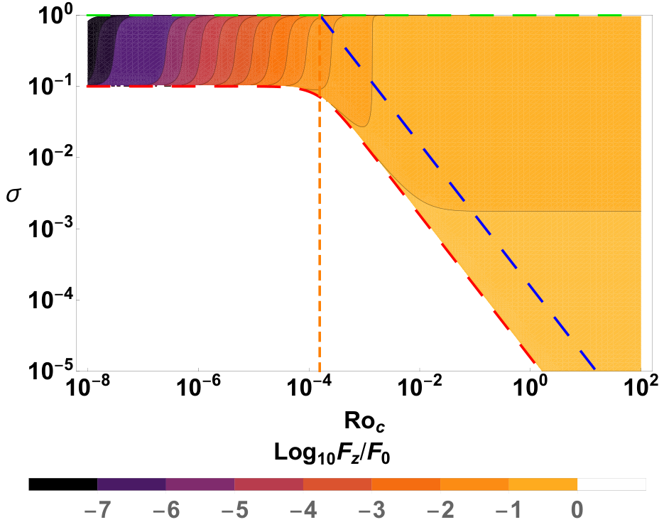
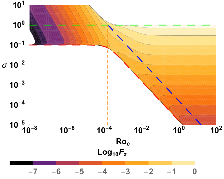
where $\mathrm{Ro_{w}}=\omega/2\Omega_{0}=5\pi\sigma\mathrm{Ro_{c}}S/\sqrt{6}$ and the wave Rossby number is $\mathrm{\widetilde{Ro}_{w}}=\mathrm{Ro_{w}}/\sqrt{\sin^{2}{\theta}\sin^{2}{\psi}+\cos^{2}{\theta}}$ .

This is depicted in Figures 2 and 3, where the colored region exhibits the magnitude of the logarithm of the energy flux ratio and the energy flux itself. An interfacial stiffness of $S=10^{3}$ is chosen as it is a rough estimate of the potential stiffness in most stars, being the ratio of the buoyancy time-scale in the stable region to the convective overturning time. The choice of latitude determines the width of the frequency band of sub-inertial waves, where it is a minimum at the pole and maximum near the equator. This is due to the presence of a critical latitude of the gravito-inertial waves, where sub-inertial waves become evanescent ( $\cos^{2}{\theta_{c}}=\mathrm{Ro_{w}}^{2}$ ). The direction of $\psi=\pm\pi/2$ is chosen as it represents the maximum value of the energy flux ratio for the choice of other parameters and represents the waves traveling toward either of the poles as the energy flux ratio is an even parity function of the horizontal direction. Specifically, the poleward wave energy flux ratio is greater than the other extremal choice of the prograde or retrograde wave energy flux ratios. In particular, given the range of $\omega_{\pm}$ , there are no sub-inertial waves in the prograde or retrograde propagation case ( $\psi=\{0,\pi\}$ , respectively), whereas the super-inertial waves may still propagate with roughly the same frequency range. The white region corresponds to the domain of evanescent waves for a given convective Rossby number with frequencies below the lower cut-off frequency ( $\sigma_{-}$ , dashed red line) for propagating GIWs. At frequencies above this threshold there is a frequency dependence of the energy flux ratio until reaching the upper cut-off where $\sigma=\omega/N_{R}=1$ , which arises due to the domain of validity when comparing GIW to gravity wave energy fluxes. Indeed, gravity waves may propagate if $\omega<N_{R}$ , whereas super-inertial GIWs may propagate even when $N_{R}<\omega<\omega_{+}$ . The transition between super-inertial and sub-inertial waves is demarked with the dashed blue line, with super-inertial waves for $\mathrm{\widetilde{Ro}_{w}}>1$ and sub-inertial waves for $\mathrm{\widetilde{Ro}_{w}}<1$ . Here, interfacially-excited super-inertial waves exhibit both a frequency and convective Rossby number dependence. Specifically, the wave energy flux decreases algebraically with frequency at a fixed convective Rossby number and have a reduced energy flux for convective Rossby numbers below unity. The interfacially-excited sub-inertial waves possess a small frequency domain at a fixed convective Rossby number over which they are propagative. The sub-inertial wave energy flux increases with decreasing convective Rossby number until a critical convective Rossby number $\mathrm{Ro}_{c,\mathrm{crit}}=\sqrt{6}/\left(5\pi S\right)$ as depicted by the vertical dashed orange line in Figure 2. Below this critical convective Rossby number, the sub-inertial wave energy flux decreases and their frequency domain is further restricted until it vanishes entirely and there are no propagative super-inertial waves . The effect of the stiffness is to lower (raise) the value of the critical convective Rossby number for larger (smaller) values of $S$ , which corresponds to the ratio of the buoyancy time-scale in the radiative zone to the convective overturning time. This may have important consequences for the wave-induced transport of angular momentum during the evolution of rotating stars. In particular, the convective Rossby number can vary by several orders of magnitude over a star’s evolution from the PMS to its ultimate demise (Landin et al. 2010; Mathis et al. 2016; Charbonnel et al. 2017, e.g.). Moreover, it can vary internally as a function of radius due to the local amplitude of the convective velocity and due to transport processes, angular momentum loss through winds, and structural changes that modify the local rotation rate (Mathis et al. 2016). Figure 4 presents the variation of the convective Rossby number at the base of the convective envelope of low-mass stars (from 0.7 to 1.5 M_⊙) throughout their evolution. These convective Rossby numbers have been calculated using grids of stellar models that take into account rotation computed with the STAREVOL code (Siess et al. 2000; Palacios et al. 2003; Decressin et al. 2009; Amard et al. 2016). The details of the micro- and macro-physics used for these grids are described in Amard et al. 2019. The dot-dashed purple line provides the value of the critical convective Rossby number ( $\mathrm{Ro}_{c,\mathrm{crit}}=\sqrt{6}/\left(5\pi S\right)$ , shown here for $S=10^{3}$ , for which an increase of the interfacial excitation of GIWs can be expected. For all the stars considered here, which have a median initial rotation (i.e. 4.5 days), this should happen during their PMS.

Figure 4: Variation of the convective Rossby number at the base of the convective envelope of low-mass stars (from 0.7 to 1.5

M_{\odot}

) along their evolution. The critical convective Rossby numbers are shown for which a potential increase of the excitation rate of GIWs (when compared to the one of pure IGWs) is expected. The purple dashed-dot line corresponds to the case of their interfacial excitation and the dashed gray line to the case of the excitation triggered by Reynolds stresses.

The flux ratio $F_{z}/F_{0}$ integrated over latitude $\theta$ , propagation direction $\psi$ , and frequency is shown in Figure 5. This illustrates the general rotational trend of the interfacial flux, namely that it decreases with increasing rotation rate. However, there is a peak at a rotational frequency that depends upon the choice of stiffness $S$ and the Rossby number of the convection at the breakup velocity $\mathrm{Ro}_{\mathrm{b}}$ . Thus, for stars with a modest rotation rate below approximately $0.2\Omega_{b}$ , the interfacial or pressure-driven GIW wave flux could play a role in transport processes that is at least as important as the transport by IGWs. Yet, for more rapidly rotating stars, this flux becomes fairly negligible due primarily to the reduction in the convective velocity amplitudes. Nevertheless, given the complex and nonanalytic form of the full integral, the exploration of the parameter dependence of this peak will be left for future work. As a means of comparison, consider the spherical Couette flow laboratory experiments of Hoff et al. 2016, where it is found that the kinetic energy of the dominant inertial mode increases with decreasing wave Rossby number. Below a critical wave Rossby number this leads to a wave breaking and an increase of small-scale structures at a critical Rossby number, which may be similar to the large increase of wave energy flux for sub-inertial waves below the critical convective Rossby number described above.

V Reynolds Stress Contributions to GIW Amplitudes

As a means of comparison, the amplitude and the wave energy flux of the GIWs may be computed exactly when using the convection model presented earlier, where the impact of rotation on the waves is treated coherently. In a means similar to Goldreich & Kumar 1990 and Lecoanet & Quataert 2013, although with a greater degree of computational complexity, one may derive the wave amplitudes for GIWs in a f-plane. As seen in Mathis et al. 2014, one must first find solutions to the homogeneous Poincaré equation for the GIWs and then use linear combinations of those solutions to construct solutions to the forced equation in the convection zone. These equations result from writing the linearized equations of motion in a f-plane as a single equation for the vertical velocity $W$ as

\displaystyle\left[\partial_{tt}\nabla^{2}+4\left(\bm{\Omega}\!\bm{\cdot}\!\bm{\nabla}\right)^{2}+N^{2}\nabla_{\perp}^{2}\right]W=\partial_{t}\mathbb{S},

(44)

where $\mathbb{S}$ is the convective source term described in detail below. Note that the thermal sources derived in Samadi & Goupil 2001 have been neglected here as in Mathis et al. 2014, for they have been found to be comparatively small for gravity waves when compared to Reynolds stresses (Belkacem et al. 2009b). In addition, the damping mechanisms (i.e. the radiative damping and the damping due to convection-wave interactions) are neglected here. As pointed out in Samadi, R. et al. 2015, the value of the amplitude of stochastically excited waves is proportional to the ratio of the energy injection rate that measures the efficiency of the couplings of turbulent motions with waves and of the damping. The focus of this work is on the energy injection rate while getting a coherent treatment of the turbulent damping of waves in rotating stars will be considered in forthcoming work.

In the stable region, where $\mathbb{S}$ is assumed to vanish, it can be shown that if one follows the methodology of constructing normal modes as in Gerkema & Shrira 2005 then the solutions of the homogeneous Poincaré equation for GIWs may be expanded as $w=\mathrm{w}(\chi,z)e^{i\omega t}$ . The horizontal coordinate $\chi=\cos{\psi}x+\sin{\psi}y$ corresponds to the distance along the direction of the wave propagation with an angle $\psi$ in the horizontal plane as seen in Gerkema & Shrira 2005 and Figure 1 of Mathis et al. 2014. Therefore, as before, the solution of the forced Poincaré equation for GIWs in the convection zone may be expanded as

	$\displaystyle W\left(\chi,z,t\right)$	$\displaystyle=\sum_{n}A_{n}\left(t\right)\mathrm{w}_{n}\left(\chi,z\right)e^{i\omega t}$		(45)
		$\displaystyle=\sum_{n}A_{n}\left(t\right)\psi_{n}\left(z\right)e^{ik_{n}\left(\chi+\delta z\right)+i\omega t},$		(46)

where $\omega$ is the chosen frequency, with $k_{n}$ being the sequence of eigenvalues associated with it, the $\psi_{n}$ are the eigenmodes of the reduced Poincaré equation (see Equation 30), and $A_{n}$ is its amplitude. Technically, the full velocity field would be an integral over all frequencies and the sum over modes associated with each frequency. However, for simplicity, this discussion will at first focus on a single frequency taken to be within the band of propagative frequencies. Substituting this into Equation 44, yields an equation for the mode amplitudes given a source function

		$\displaystyle\sum_{n}\left\{\left[\partial_{tt}A_{n}+2i\omega\partial_{t}A_{n}\right]\left[\partial_{zz}-k_{n}^{2}\right]+A_{n}\left[\left(f^{2}-\omega^{2}\right)\partial_{zz}\right.\right.$
		$\displaystyle\left.\left.+2iff_{ss}k_{n}\partial_{z}+k_{n}^{2}\left(\omega^{2}-N^{2}-f_{ss}^{2}\right)\right]\right\}\mathrm{w}_{n}e^{i\omega t}=\partial_{t}\mathbb{S}.$		(47)

Noting that the second term is simply the homogeneous equation, it vanishes, leaving

$\displaystyle\sum_{n}$	$\displaystyle\left[\partial_{tt}A_{n}+2i\omega\partial_{t}A_{n}\right]$
	$\displaystyle\times\left[\partial_{zz}\psi_{n}+2ik_{n}\delta\partial_{z}\psi_{n}-k_{n}^{2}\left(\delta^{2}+1\right)\psi_{n}\right]$
	$\displaystyle\times e^{ik_{n}\left(\chi+\delta z\right)+i\omega t}=\partial_{t}\mathbb{S}.$	(48)

Utilizing Equation 30, this becomes

		$\displaystyle\sum_{n}\left[\partial_{tt}A_{n}+2i\omega\partial_{t}A_{n}\right]$
		$\displaystyle\times\!\!\left[2ik_{n}\delta\partial_{z}\psi_{n}-k_{n}^{2}\!\!\left(\!\!\frac{f^{2}-N^{2}}{f^{2}-\omega^{2}}+\frac{\left(\omega^{2}+f^{2}\right)f_{ss}^{2}}{\left(f^{2}-\omega^{2}\right)^{2}}\!\!\right)\!\!\psi_{n}\right]$
		$\displaystyle\times e^{ik_{n}\left(\chi+\delta z\right)+i\omega t}=\partial_{t}\mathbb{S}.$		(49)

Assuming homogeneous Dirichlet boundary conditions on $\psi_{n}$ and that the change in the amplitudes at infinity are zero, with an initial condition of being zero, this can be integrated against a single conjugate mode of index $m$ to see that the constant amplitude is

\displaystyle\langle A_{n}\rangle

\displaystyle=\frac{i\int_{0}^{L}dz\int_{-\infty}^{\infty}d\chi\int_{-\infty}^{\infty}dt\partial_{t}\mathbb{S}\psi_{n}^{*}e^{-ik_{n}\left(\chi+\delta z\right)-i\omega t}}{2\omega k_{n}^{2}\int_{0}^{L}dz\left(\frac{f^{2}-N^{2}}{f^{2}-\omega^{2}}+\frac{\left(\omega^{2}+f^{2}\right)f_{ss}^{2}}{\left(f^{2}-\omega^{2}\right)^{2}}\right)\left|\psi_{n}\right|^{2}},

(50)

where the normalization $c_{n}$ follows from the orthogonality condition on the $\psi_{n}$ ,

\displaystyle c_{n}^{2}\delta_{nm}=\frac{1}{L}\int_{0}^{L}dz\left(\frac{\omega^{2}-N^{2}}{f^{2}-\omega^{2}}+\frac{\omega^{2}f_{ss}^{2}}{\left(f^{2}-\omega^{2}\right)^{2}}\right)\psi_{m}^{*}\psi_{n}.

(51)

where $L=z_{2}-z_{1}$ is the depth of the domain. The convective source term is

\displaystyle\mathbb{S}

\displaystyle=\partial_{z}\bm{\nabla}\bm{\cdot}{\mathbf{F}}-\nabla^{2}F_{z}=\partial_{z}\bm{\nabla}_{\perp}\bm{\cdot}\mathbf{F}-\nabla_{\perp}^{2}F_{z},

(52)

where $\mathbf{F}=\bm{\nabla}\bm{\cdot}{\left(\bm{v}\otimes\bm{v}\right)}$ are the Reynolds stresses due to the convective velocities $\bm{v}$ . This can be further simplified noting the definition of the perpendicular direction, yielding

	$\displaystyle\mathbb{S}$	$\displaystyle=\partial_{\chi z}F_{\chi}-\partial_{\chi}^{2}F_{z},$		(53)
		$\displaystyle=\partial_{\chi\chi z}\left(v_{\chi}^{2}-v_{z}^{2}\right)+\left(\partial_{\chi zz}-\partial_{\chi\chi\chi}\right)v_{\chi}v_{z}.$		(54)

The integral in the numerator of Equation 50 can be identified as a Fourier transform of the source in time and space. Treating it as such, it becomes

		$\displaystyle\int_{0}^{L}dz\int_{-\infty}^{\infty}d\chi\int_{-\infty}^{\infty}dt\partial_{t}\mathbb{S}\psi_{n}^{*}e^{-ik_{n}\left(\chi+\delta z\right)-i\omega t}$
		$\displaystyle=\!\omega\!\!\int_{0}^{L}\!\!dz\!\left[ik_{n}^{2}\partial_{z}\!\left(\widetilde{v_{z}^{2}\,}\!-\!\widetilde{v_{\chi}^{2}}\right)\!-\!k_{n}\!\left(\partial_{zz}\!+\!k_{n}^{2}\right)\!\widetilde{v_{\chi}v_{z}}\right]\!\psi_{n}^{*}e^{-ik_{n}\delta z}.$		(55)

In turn this is a Fourier transform of a product, or a convolution in spectral space of the Reynolds stress with a Heaviside function $H$ that confines the convection to a the convective region and the reduced eigenmodes. Under this approach, the previous equation yields

		$\displaystyle\omega\int_{-\infty}^{\infty}dk^{\prime}\left[k^{\prime}k_{n}^{2}\left(\widehat{v_{z}^{2}\,}\left(k^{\prime}\right)-\widehat{v_{\chi}^{2}}\left(k^{\prime}\right)\right)\right.$
		$\displaystyle\left.+k_{n}\left(k^{\prime 2}-k_{n}^{2}\right)\widehat{v_{\chi}v_{z}}\left(k^{\prime}\right)\right]\widehat{H\psi_{n}^{*}}\left(k_{n}\delta-k^{\prime}\right).$		(56)

Assuming henceforth that the Brunt-Väisälä frequency is a discontinuous jump of an amplitude $N=S\omega_{c}$ , there is an exact solution for all three wave classes, sub-inertial, inertial, and super-inertial. This assumption provides an approximation of the stratification in a star, but captures its order of magnitude effects. This means that all integrals except the one of the Reynolds stresses can be evaluated. The latter depends upon the turbulence model that is chosen. The one introduced at the beginning of this paper will be examined here. Specifically, with this choice of $N$ , the reduced Poincaré equation becomes

\displaystyle\left\{\begin{array}[]{lr}\partial_{zz}\psi_{n}+k_{n}^{2}\alpha^{2}\psi_{n}=0&0\leq z<\ell_{s}\\ \partial_{zz}\psi_{n}+k_{n}^{2}\beta^{2}\psi_{n}=0&\ell_{s}\leq z\leq L\end{array}\right.,

where

	$\displaystyle\alpha^{2}$	$\displaystyle=\frac{N^{2}-\omega^{2}}{\omega^{2}-f^{2}}+\frac{\omega^{2}f_{ss}^{2}}{\left(\omega^{2}-f^{2}\right)^{2}},$		(59)
	$\displaystyle\beta^{2}$	$\displaystyle=\frac{\omega^{2}f_{ss}^{2}}{\left(\omega^{2}-f^{2}\right)^{2}}-\frac{\omega_{c}^{2}+\omega^{2}}{\omega^{2}-f^{2}},$		(60)

and where $\omega_{c}$ is the convective overturning time and $\ell_{s}=z_{c}-z_{1}$ is the depth of the radiative-convective interface. The boundary conditions are that $\psi_{n}(0)=\psi_{n}(L)=0$ , and with matching conditions and momentum continuity at the interface leading to the dispersion relationship. With these choices, above equations admit the following solutions for the sub-inertial waves

\displaystyle\psi_{n}=\left\{\begin{array}[]{lr}-\displaystyle{\frac{\sin\left(k_{n}\beta\left(L-\ell_{s}\right)\right)}{\cos\left(k_{n}\beta L\right)\sin\left(k_{n}\alpha\ell_{s}\right)}\sin\left(k_{n}\alpha z\right)}&0\leq z<\ell_{s}\\ \sin\left(k_{n}\beta z\right)-\tan\left(k_{n}\beta L\right)\cos\left(k_{n}\beta z\right)&\ell_{s}\leq z\leq L\end{array}\right.,

with a dispersion relationship

\displaystyle\alpha\tan\left[k_{n}\beta\left(L-\ell_{s}\right)\right]+\beta\tan\left[k_{n}\alpha\ell_{s}\right]=0.

(63)

Similarly, the super-inertial waves are

\displaystyle\psi_{n}=\left\{\begin{array}[]{lr}-\displaystyle{\frac{\sinh\left(k_{n}\beta\left(L-\ell_{s}\right)\right)}{\cosh\left(k_{n}\beta L\right)\sin\left(k_{n}\alpha\ell_{s}\right)}\sin\left(k_{n}\alpha z\right)}&0\leq z<\ell_{s}\\ \sinh\left(k_{n}\beta z\right)-\tanh\left(k_{n}\beta L\right)\cosh\left(k_{n}\beta z\right)&\ell_{s}\leq z\leq L\end{array}\right.,

with a dispersion relationship

\displaystyle\alpha\tanh\left[k_{n}\beta\left(L-\ell_{s}\right)\right]+\beta\tan\left[k_{n}\alpha\ell_{s}\right]=0.

(66)

Note that with $\sin\left(k_{n}\alpha\ell_{s}\right)$ in the numerator, there are certain values of $k_{n}\alpha\ell_{s}=m\pi$ with $m$ some integer where this solution is invalid. This provides an additional selection criterion on the values of S that have solutions. Note that the inertial waves already are normalized with $c_{n}=1$ . The integrals for the denominator in Equation 50 are very similar.

Finally, from Equation 62 in André et al. 2017, the vertical wave flux for a single mode is given as

\displaystyle F_{z}=\frac{\rho_{0}}{2}\left(\frac{f^{2}-\omega^{2}}{\omega k_{n}^{2}}\right)\left|A_{n}^{2}\psi_{n}\partial_{z}\psi_{n}\right|.

(67)

Note that this definition of the flux is slightly different from the interfacial flux, which used an approximation of the pressure. Moreover, that interfacial flux is a local model with driving taking place only at the interface, whereas the current model assesses wave driving throughout the convective zone. The definition of the flux given in Equation 67 is consistent with previous studies of gravity wave driving in the bulk of convective regions (Press 1981; Goldreich & Kumar 1990; Lecoanet & Quataert 2013, e.g.,), where it is seen that the flux for a discontinuous Brunt-Väisälä frequency is $F_{z}\approx F_{c}S^{-1}$ , where $F_{c}$ is the convective flux. This scaling can be obtained using Equation 67 if one considers the regime of low-frequency gravity waves in the non-rotating case (where $f=0$ ), which are described within the JWKB approximation, assuming that their horizontal velocity is $v_{h}\approx v_{c}=\omega_{c}/k_{c}$ , where $v_{c}$ , $\omega_{c}$ , and $k_{c}$ are the convective velocity, frequency, and wavevector, respectively, while one also sets $\omega\approx\omega_{c}$ and $k\approx k_{c}$ . Note that within these assumptions the influence of the spatial behaviour of the eigenmodes is not taken into account.

Thus, with the definition of the amplitude, the flux is

		$\displaystyle F_{z}=\frac{\rho_{0}\left(f^{2}-\omega^{2}\right)\left\|\psi_{n}\partial_{z}\psi_{n}\right\|}{8\omega^{3}k_{n}^{6}}$
		$\displaystyle\times\frac{\left\|\int_{0}^{L}dz\int_{-\infty}^{\infty}d\chi\int_{-\infty}^{\infty}dt\partial_{t}\mathbb{S}\psi_{n}^{*}e^{-ik_{n}\left(\chi+\delta z\right)-i\omega t}\right\|^{2}}{\left(\int_{0}^{L}dz\displaystyle{\left(\frac{f^{2}-N^{2}}{f^{2}-\omega^{2}}+\frac{\left(\omega^{2}+f^{2}\right)f_{ss}^{2}}{\left(f^{2}-\omega^{2}\right)^{2}}\right)}\left\|\psi_{n}\right\|^{2}\right)^{2}}.$		(68)

Averaging over the stable region, this becomes

		$\displaystyle F_{z}=\frac{\rho_{0}\left(f^{2}-\omega^{2}\right)\psi_{n}^{2}(\ell_{s})}{8\omega^{3}k_{n}^{6}\ell_{s}}$
		$\displaystyle\times\frac{\left\|\int_{0}^{L}dz\int_{-\infty}^{\infty}d\chi\int_{-\infty}^{\infty}dt\partial_{t}\mathbb{S}\psi_{n}^{*}e^{-ik_{n}\left(\chi+\delta z\right)-i\omega t}\right\|^{2}}{\left(\int_{0}^{L}dz\displaystyle{\left(\frac{f^{2}-N^{2}}{f^{2}-\omega^{2}}+\frac{\left(\omega^{2}+f^{2}\right)f_{ss}^{2}}{\left(f^{2}-\omega^{2}\right)^{2}}\right)}\left\|\psi_{n}\right\|^{2}\right)^{2}}.$		(69)

The integral in the denominator of the wave flux for the sub-inertial and super-inertial waves are thus

		$\displaystyle D_{n}=\sec^{4}\left(k_{n}L\beta\right)$
		$\displaystyle\times\!\!\left[\frac{\sin^{2}\!\left(k_{n}\beta\ell_{0}\right)}{\sin^{2}\left(k_{n}\alpha\ell_{s}\right)}\!\left(\!\frac{f^{2}-N^{2}}{f^{2}-\omega^{2}}+\frac{\left(\omega^{2}+f^{2}\right)f_{ss}^{2}}{\left(f^{2}-\omega^{2}\right)^{2}}\!\right)\right.$
		$\displaystyle\qquad\times\left(\frac{\ell_{s}}{2}\!-\!\frac{\sin\left(2k_{n}\alpha\ell_{s}\right)}{4k_{n}\alpha}\right)$
		$\displaystyle\left.+\left(\!\frac{f^{2}+\omega_{c}^{2}}{f^{2}-\omega^{2}}+\frac{\left(\omega^{2}+f^{2}\right)f_{ss}^{2}}{\left(f^{2}-\omega^{2}\right)^{2}}\!\right)\left(\frac{\ell_{0}}{2}-\frac{\sin\left(2k_{n}\beta\ell_{0}\right)}{4k_{n}\beta}\right)\right]^{2}\!\!\!\!,$		(70)

for the sub-inertial waves and

		$\displaystyle D_{n}=\mathrm{sech}^{4}\left(k_{n}L\beta\right)$
		$\displaystyle\times\!\!\left[\frac{\sinh^{2}\!\left(k_{n}\beta\ell_{0}\right)}{\sin^{2}\left(k_{n}\alpha\ell_{s}\right)}\!\left(\!\frac{f^{2}-N^{2}}{f^{2}-\omega^{2}}+\frac{\left(\omega^{2}+f^{2}\right)f_{ss}^{2}}{\left(f^{2}-\omega^{2}\right)^{2}}\!\right)\right.$
		$\displaystyle\qquad\times\left(\frac{\ell_{s}}{2}\!-\!\frac{\sin\left(2k_{n}\alpha\ell_{s}\right)}{4k_{n}\alpha}\right)$
		$\displaystyle\left.+\left(\!\frac{f^{2}+\omega_{c}^{2}}{f^{2}-\omega^{2}}+\frac{\left(\omega^{2}+f^{2}\right)f_{ss}^{2}}{\left(f^{2}-\omega^{2}\right)^{2}}\!\right)\left(\frac{\ell_{0}}{2}+\frac{\sinh\left(2k_{n}\beta\ell_{0}\right)}{4k_{n}\beta}\right)\right]^{2}\!\!\!\!,$		(71)

for the super-inertial waves.

The integral in the numerator can be computed exactly for the convection model discussed in Section II. Specifically, using the definition of the velocities there, e.g.

	$\displaystyle\mathrm{v}_{z}$	$\displaystyle=\mathrm{v}\left(\mathrm{Ro_{c}}\right)\sin{\left(\frac{\pi z}{\ell_{0}}\right)}e^{\left(ik_{\perp}\chi+i\omega_{c}t\right)},$		(72)
	$\displaystyle\mathrm{v}_{\chi}$	$\displaystyle=\frac{i\pi}{\ell_{0}k_{\perp}}\mathrm{v}\left(\mathrm{Ro_{c}}\right)\cos{\left(\frac{\pi z}{\ell_{0}}\right)}e^{\left(ik_{\perp}\chi+i\omega_{c}t\right)},$		(73)

as follows from the continuity equation for the convection model. These integrals are

		$\displaystyle\frac{\pi^{4}v^{4}\sec^{2}\left(2k_{\perp}L\beta\right)\left(2k_{\perp}^{2}\ell_{0}^{2}-3\pi^{2}\right)^{2}}{2\ell_{0}^{4}\left[\pi^{4}-2\pi^{2}k_{\perp}^{2}\ell_{0}^{2}\left(\beta^{2}+\delta^{2}\right)+k_{\perp}^{4}\ell_{0}^{4}\left(\beta^{2}-\delta^{2}\right)^{2}\right]^{2}}$
		$\displaystyle\times\left[\pi^{4}-2\pi^{2}k_{\perp}^{2}\ell_{0}^{2}\left(\beta^{2}+\delta^{2}\right)+k_{\perp}^{4}\ell_{0}^{4}(\beta^{4}+14\beta^{2}\delta^{2}+\delta^{4})\right.$
		$\displaystyle+4\beta\delta k_{\perp}^{2}\ell_{0}^{2}\left(k_{\perp}^{2}\ell_{0}^{2}\left(\beta-\delta\right)^{2}-\pi^{2}\right)$
		$\displaystyle\qquad\times\left(\cos\left(2k_{\perp}\ell_{0}\left(\beta+\delta\right)\right)+\cos\left(2k_{\perp}\ell_{0}\left(\beta-\delta\right)\right)\right)$
		$\displaystyle\left.-\!\left(\pi^{2}\!-\!k_{\perp}^{2}\ell_{0}^{2}\left(\beta+\delta\right)^{2}\right)\!\!\left(\pi^{2}\!-\!k_{\perp}^{2}\ell_{0}^{2}\left(\beta\!-\!\delta\right)^{2}\right)\!\cos\left(4k_{\perp}\ell_{0}\beta\right)\right],$		(74)

for the sub-inertial waves where the horizontal and time integrals impose $\omega=2\omega_{c}$ and $k_{\perp}=k_{n}/2$ . For the super-inertial waves, this is

		$\displaystyle-\frac{\pi^{4}v^{4}\mathrm{sech}^{2}\left(k_{\perp}L\beta\right)\left(2k_{\perp}^{2}\ell_{0}^{2}-3\pi^{2}\right)^{2}}{2\ell_{0}^{4}\left[\pi^{4}+2\pi^{2}k_{\perp}^{2}\ell_{0}^{2}\left(\beta^{2}-\delta^{2}\right)+k_{\perp}^{4}\ell_{0}^{4}\left(\beta^{2}+\delta^{2}\right)^{2}\right]^{2}}$
		$\displaystyle\times\left[\pi^{4}+2\pi^{2}k_{\perp}^{2}\ell_{0}^{2}\left(\beta^{2}-\delta^{2}\right)+k_{\perp}^{4}\ell_{0}^{4}(\beta^{4}-14\beta^{2}\delta^{2}+\delta^{4})\right.$
		$\displaystyle+16\beta^{2}\delta^{2}k_{\perp}^{4}\ell_{0}^{4}\cos\left(2k_{\perp}\ell_{0}\delta\right)\cosh\left(2k_{\perp}\ell_{0}\beta\right)$
		$\displaystyle-8\beta\delta k_{\perp}^{2}\ell_{0}^{2}\left(\pi^{2}+k_{\perp}^{2}\ell_{0}^{2}\left(\beta^{2}-\delta^{2}\right)\right)$
		$\displaystyle\qquad\times\sin\left(2k_{\perp}\ell_{0}\delta\right)\sinh\left(2k_{\perp}\ell_{0}\beta\right)$
		$\displaystyle-\!\left(k_{\perp}^{2}\ell_{0}^{2}\beta^{2}+\left(\pi+k_{\perp}\ell_{0}\delta\right)^{2}\right)$
		$\displaystyle\left.\qquad\times\left(k_{\perp}^{2}\ell_{0}^{2}\beta^{2}+\left(\pi-k_{\perp}\ell_{0}\delta\right)^{2}\right)\!\cosh\left(4k_{\perp}\ell_{0}\beta\right)\right].$		(75)

These waves will attain a maximum flux near the equator, especially for low convective Rossby number where the waves become increasingly equatorially focused. Thus, evaluating these expressions at the equator, one has a wave flux analogous to the section on interfacial waves, but excited by the Reynolds stresses in the bulk of the convection zone. Figure 6 illustrates this flux for several values of the stiffness, where each value of the convective Rossby number is computed such that the dispersion relationships are obeyed, leading to its discrete nature. The sub-inertial waves have an oscillatory character, where some waves achieve a resonance and have a peak in flux. The peak flux arises at moderate convective Rossby numbers below $1/\sqrt{5}$ , due to $\alpha$ being small and transitioning from super-inertial to sub-inertial waves. The decay of the flux at lower convective Rossby numbers results from the weakening convective velocities and the increasing horizontal wavenumber of the convection. The peak in the super-inertial waves also occurs near $\mathrm{Ro}_{c}=1/\sqrt{5}$ , above which it decays primarily due to the scaling of the denominator of the flux, which arises from the hyperbolic trigonometric functions in the structure of the eigenmodes and it asymptotes to the flux of pure gravity waves driven by nonrotating convection. When considering Figure 4 and also Figure 4 in Mathis et al. 2016, where $\mathrm{Ro_{c}}=1/\sqrt{5}$ is distinguished by the dashed gray line. One can see that these phenomena may occur for a majority of low-mass stars along their evolution, in particular during the PMS (or close to the base of their convective envelope) because of the low values of $\mathrm{Ro}_{c}$ during these evolutionary phases (and in these regions).

The actual value of the both the nonrotating and rotating fluxes are very dependent upon the value of the stiffness chosen due to the dependence on the average of the eigenfunction in the stable region in the numerator and the normalization in the denominator of the flux derived above. The non-rotating wave flux normalized by the total convective flux is shown in Figure 6(d). Note that this flux $F_{0}$ differs from that of Section IV because the flux defined in Equation 67 has a complex spatial dependence. When averaged over the stable region, this yields $F_{0}\propto Q(S)S^{-4}$ where $Q(S)$ is the dependence arising from the integral of the source term and the average value of $|\psi_{n}\partial_{z}\psi_{n}|$ in the radiative region (see Equation 68). However, if one makes the assumptions explained in the Appendix, where the spatial dependence of the eigenfunctions and their dispersion relationship become simple and continuous (see Appendix), one recovers $F_{0}\propto S^{-1}$ . Thus, if one makes similar assumptions for the gravito-inertial waves, then $F_{z}/F_{0}\propto 1$ , whereas with the more complex spatial dependence of the exact eigenfunctions and the more intricate dispersion relationship it scales as $F_{z}/F_{0}\propto Q(S)S^{-2}$ as seen in Figure 6. Finally, both the flux of the IGWs and the GIWs are always weaker than the total convective flux.

VI Summary and Discussion

A model of rotating convection originating with Stevenson 1979 has been extended to include thermal and viscous diffusions for any convective Rossby number in Augustson & Mathis 2019. The scaling of the velocity and superadiabaticity in terms of the colatitude, and Rossby number are outlined in Section II. Asymptotically at low convective Rossby number and without diffusion, these match the expressions given in Stevenson 1979, as well as the numerical results found in the 3D simulations of Käpylä et al. 2005 and Barker et al. 2014.

Here this rotating convection model has been employed to examine the excitation of gravito-inertial waves (GIWs) by two different channels: one by interfacial excitation and another by Reynolds-stress excitation. First, the convection model is applied to the interfacial wave excitation paradigm developed in Press 1981, where the gravity wave dynamics there is replaced with the GIW wave dynamics computed in Mathis et al. 2014 and André et al. 2017. Both mechanisms are considered since, as seen in Lecoanet et al. 2015, both sources of wave excitation play a role in simulations of gravity wave excitation, with the dominant one being due to the volume integrated Reynolds stresses. Next, with a turbulent convective velocity spectrum in hand, more sophisticated approaches allow for the computation of the wave energy flux in the context of both more realistic variations in the Brunt-Väisälä frequency as well as in a non-interfacial paradigm that includes the Reynolds stresses throughout the convection zone. Such a step has been taken in this paper, which builds upon the methods developed in Belkacem et al. 2009a, Lecoanet & Quataert 2013, Mathis et al. 2014, where the gravity wave and GIW excitation amplitudes and accompanying wave energy injection rate are computed by solving the wave equation driven by a convective source term. This approach provides a general method of computing the wave flux that takes into account the volumetric excitation of the waves and that includes the region in which they are potentially evanescent. Specifically, to assess the influence of the convective Reynolds stresses and of rotation on the GIWs, a wave energy flux estimate is constructed using an explicit computation of the amplitude for both the super-inertial and sub-inertial waves. The convection model of Paper I is then invoked as means of estimating the Reynolds stresses.

In the context of the wave energy flux, distinct parameter regimes have been found that depend upon the mode of excitation (either interfacial pressure perturbations or convective Reynolds stresses), the convective Rossby number (or alternatively the rotation rate), and the stiffness of the convective-radiative interface. The visibility of these regimes depends upon the colatitude selected, with the distinction between them being starkest at low latitudes near the equator and vanishing at the poles due to impact of the Coriolis acceleration on the frequency range over which GIWs may propagate. As depicted in Figure 2, interfacially-excited sub-inertial waves have a peak energy flux near a critical convective Rossby number, but decay below it. Interfacially-excited super-inertial waves, on the other hand, have an increasing energy flux with increasing frequency and increasing Rossby number. As a means of comparison, the influence of convective Reynolds stresses on the wave amplitude and their energy flux has been assessed by directly employing the convection model of Paper I. The detailed behavior of the eigenfunctions appropriate for GIWs and how they interact with the convective source is examined in V. A trend similar to that of interfacial waves is found where there is a decline in the amplitude of the fluxes is found as the convective Rossby number is decreased for both the sub and super-inertial waves. However, there is a large variation in the sub-inertial wave flux for a given convective Rossby number, depending upon whether wave is in resonance or not, leading to the series of peaks seen in Figure 6 where the flux relative to gravity waves in nonrotating convection can be many orders of magnitude larger, but still below the convective flux. The amplitude of the nonrotating flux is computed using the same mathematical formalism as the gravito-inertial waves, but utilizing the proper eigenmodes. The super-inertial waves have an increased flux at lower Rossby numbers reaching a peak at the transitional Rossby number of $1/\sqrt{5}$ for the parameters chosen in Figure 6.

If realized, these characteristics of GIWs may have substantial consequences for the transport and mixing of angular momentum, chemical species, and heat in stellar and planetary interiors, in particular during the PMS of low-mass stars or close to the base of their convective envelope, as well as consequences for the seismic observations of them. According to the results presented in §IV and shown in Figure 2, the GIW energy flux due to interfacially-excited waves is likely to be reduced relative to the nonrotating case when the wave Rossby number is not close to the critical one, meaning that any transport mechanisms associated with those waves will be reduced as well. Similarly, as discussed in §V and shown in Figure 6, the sub-inertial wave energy flux generally decreases at lower convective Rossby numbers, but reaches a peak at moderate Rossby number. What is described here is the energy injection rate by turbulent convective motions into GIWs. However, to get a more complete picture, the damping of GIWs resulting from their interactions with turbulent convection needs to be studied (see Samadi & Goupil 2001 and Belkacem et al. 2009a). Nevertheless, the examination of Be star outbursts in Neiner et al. 2020 have already pointed to tantilizing clues about the role of gravito-inertial waves in angular momentum transport. There, a global description of gravito-inertial wave excitation is employed to compute the a wave spectrum that matches the observations well (see their Figure 7).

Finally, the model examined here for the wave energy flux and excitation of GIWs has assumed a particular form of the convective Reynolds stresses that is valid only in local domains. However, this neglects global-scale shearing flows seen in 3D convection simulations in spherical geometry (Brun et al. 2011; Augustson et al. 2012; Alvan et al. 2015; Emeriau-Viard & Brun 2017, e.g.,) and theoretically predicted (Busse 2002; Julien et al. 2006; Grooms et al. 2010), as well as neglecting the more extremal convective events that can still occur frequently enough to influence the wave energy flux (Pratt et al. 2017b; Pratt et al. 2017a, e.g.,). These events have typically been modeled as collections of plumes for gravity waves (Schmitt et al. 1984; Schatzman 1993; Schatzman 1996; Pinçon et al. 2016; Pinçon et al. 2017, e.g.,), and they are tied closely to the interfacial excitation model as such events are more likely to deform the average interface depth at least in the local region near the plume. Therefore, the model can be further improved by considering more sophisticated models of the structure of the flows, such as applying the models of rotating plumes considered in Pedley 1968 or Grooms et al. 2010. Thus, the formalism developed here will be extended in future work to include the influence of rotation on those plumes as well as a utilizing theoretical models for global-scale flows to better characterize GIW excitation and energy flux.

Acknowledgments

The authors thank the referee for their very careful reading of the manuscript and their helpful and constructive comments. K. C. Augustson, S. Mathis, and A. Astoul acknowledge support from the ERC SPIRE 647383 grant and PLATO CNES grant at CEA/DAp-AIM. The authors also thank Q. André, U. Lee, C. Neiner, C. Pinçon, and V. Prat for fruitful conversations.

Appendix A Gravity Wave Flux in the Nonrotating and Low-Frequency Limit

With the appropriate limit and the assumptions made in Goldreich & Kumar 1990 and Lecoanet & Quataert 2013, which also are similar to those made in section 4 of this paper and in Press 1981, one can show that they are equivalent. To do this, recall that the definition of the flux given in Equation 67 is

F_{z}=\rho_{0}\frac{f^{2}-\omega^{2}}{2\omega k_{n}^{2}}\left|A_{n}^{2}\psi_{n}\partial_{z}\psi_{n}\right|.

(A1)

In the non-rotating limit this becomes

F_{z}=-\rho_{0}\frac{\omega}{2k_{n}^{2}}|A_{n}^{2}\psi_{n}\partial_{z}\psi_{n}|.

(A2)

In the asymptotic limit of low-frequency gravity waves the JWKB approximation can be applied where $\partial_{z}\psi_{n}\approx ik_{V}\psi_{n}$ , so the flux becomes

F_{z}=-\rho_{0}\frac{\omega k_{V}}{2k_{n}^{2}}|A_{n}\psi_{n}|^{2}.

(A3)

In this limit, the vertical wavenumber is approximately

k_{V}=\frac{N}{\omega}k_{n}.

(A4)

So, then it can be seen that

F_{z}=-\rho_{0}\frac{N}{2k_{n}}|A_{n}|^{2}\psi_{n}^{2}.

(A5)

Now, noting that $v_{w}=A_{n}\psi_{n}$ is the vertical velocity of the wave, one has that

F_{z}=-\rho_{0}\frac{N}{2k_{n}}v_{w}^{2}.

(A6)

Making the assumptions of Goldreich & Kumar 1990, Lecoanet & Quataert 2013, and Press 1981, one has that $k_{n}\approx k_{c}$ , $\omega\approx\omega_{c}$ and $v_{w}\approx\omega_{c}^{2}/(k_{c}N)$ , where the subscript $c$ indicates the wave vector ( $k_{c}$ ) and overturning frequency ( $\omega_{c}$ ) of the convection. To obtain this expression of $v_{w}$ , we consider the low-frequency regime where the ratio between the vertical and the horizontal components of the gravity waves’ velocity is given approximately by $v_{w}/v_{h}\approx\omega/N$ . In addition, it is assumed, as in Equation (36) of Press 1981 and in Equation (49) of Lecoanet & Quataert 2013, that the horizontal wave velocity is given by $v_{h}\approx v_{c}=\omega_{c}/k_{c}$ . Therefore, the previous expression becomes

F_{z}\approx-\rho_{0}\frac{N}{2k_{c}}\left(\frac{\omega_{c}^{2}}{k_{c}N}\right)^{2}=-\rho_{0}\frac{\omega_{c}^{4}}{2k_{c}^{3}N}.

(A7)

Now, since $u_{c}=\omega_{c}/k_{c}$ (the convective velocity), one has that

F_{z}\propto\rho_{0}u_{c}^{3}\frac{\omega_{c}}{2N}\propto F_{c}M,

(A8)

where $M=\omega_{c}/N=S^{-1}$ is the Mach number or the inverse stiffness ( $S$ ) and $F_{c}$ is the convective flux. Hence, under these limits and assumptions, the flux definitions have the same scaling. Note that within these assumptions the influence of the spatial behaviour of the eigenmodes is not apparent because $|\psi_{n}|^{2}\approx|e^{ik_{V}z}|^{2}=1$ , which is not the case for the exact solutions used in Equation 68.

References

Aerts et al. (2010) Aerts, C., Christensen-Dalsgaard, J., & Kurtz, D. W. 2010, Asteroseismology
Aerts et al. (2018) Aerts, C., Mathis, S., & Rogers, T. 2018, arXiv e-prints. https://arxiv.org/abs/1809.07779
Aerts et al. (2017) Aerts, C., Van Reeth, T., & Tkachenko, A. 2017, ApJ, 847, L7, doi: 10.3847/2041-8213/aa8a62
Aerts et al. (2019) Aerts, C., Pedersen, M. G., Vermeyen, E., et al. 2019, A&A, 624, A75, doi: 10.1051/0004-6361/201834762
Alexakis & Biferale (2018) Alexakis, A., & Biferale, L. 2018, Phys. Rep., 767, 1, doi: 10.1016/j.physrep.2018.08.001
Alvan et al. (2014) Alvan, L., Brun, A. S., & Mathis, S. 2014, A&A, 565, A42, doi: 10.1051/0004-6361/201323253
Alvan et al. (2013) Alvan, L., Mathis, S., & Decressin, T. 2013, A&A, 553, A86, doi: 10.1051/0004-6361/201321210
Alvan et al. (2015) Alvan, L., Strugarek, A., Brun, A. S., Mathis, S., & Garcia, R. A. 2015, A&A, 581, A112, doi: 10.1051/0004-6361/201526250
Amard et al. (2016) Amard, L., Palacios, A., Charbonnel, C., Gallet, F., & Bouvier, J. 2016, A&A, 587, A105, doi: 10.1051/0004-6361/201527349
Amard et al. (2019) Amard, L., Palacios, A., Charbonnel, C., et al. 2019, A&A, 631, A77, doi: 10.1051/0004-6361/201935160
Ando et al. (2018) Ando, H., Takagi, M., Fukuhara, T., et al. 2018, Journal of Geophysical Research (Planets), 123, 2270, doi: 10.1029/2018JE005640
André et al. (2017) André, Q., Barker, A. J., & Mathis, S. 2017, A&A, 605, A117, doi: 10.1051/0004-6361/201730765
Augustson et al. (2012) Augustson, K. C., Brown, B. P., Brun, A. S., Miesch, M. S., & Toomre, J. 2012, ApJ, 756, 169, doi: 10.1088/0004-637X/756/2/169
Augustson et al. (2016) Augustson, K. C., Brun, A. S., & Toomre, J. 2016, ApJ, 829, 92, doi: 10.3847/0004-637X/829/2/92
Augustson & Mathis (2019) Augustson, K. C., & Mathis, S. 2019, ApJ, 874, 83, doi: 10.3847/1538-4357/ab0b3d
Barker et al. (2014) Barker, A. J., Dempsey, A. M., & Lithwick, Y. 2014, ApJ, 791, 13, doi: 10.1088/0004-637X/791/1/13
Beck et al. (2012) Beck, P. G., Montalban, J., Kallinger, T., et al. 2012, Nature, 481, 55, doi: 10.1038/nature10612
Belkacem et al. (2009a) Belkacem, K., Mathis, S., Goupil, M. J., & Samadi, R. 2009a, A&A, 508, 345, doi: 10.1051/0004-6361/200912284
Belkacem et al. (2009b) Belkacem, K., Samadi, R., Goupil, M. J., et al. 2009b, A&A, 494, 191, doi: 10.1051/0004-6361:200810827
Benomar et al. (2015) Benomar, O., Takata, M., Shibahashi, H., Ceillier, T., & García, R. A. 2015, MNRAS, 452, 2654, doi: 10.1093/mnras/stv1493
Browning et al. (2004) Browning, M. K., Brun, A. S., & Toomre, J. 2004, ApJ, 601, 512, doi: 10.1086/380198
Brun et al. (2011) Brun, A. S., Miesch, M. S., & Toomre, J. 2011, ApJ, 742, 79, doi: 10.1088/0004-637X/742/2/79
Brun et al. (2017) Brun, A. S., Strugarek, A., Varela, J., et al. 2017, ApJ, 836, 192, doi: 10.3847/1538-4357/aa5c40
Busse (2002) Busse, F. H. 2002, Ph. Fl., 14, 1301, doi: 10.1063/1.1455626
Charbonnel et al. (2013) Charbonnel, C., Decressin, T., Amard, L., Palacios, A., & Talon, S. 2013, A&A, 554, A40, doi: 10.1051/0004-6361/201321277
Charbonnel et al. (2017) Charbonnel, C., Decressin, T., Lagarde, N., et al. 2017, A&A, 605, A102, doi: 10.1051/0004-6361/201526724
Christophe et al. (2018) Christophe, S., Ballot, J., Ouazzani, R. M., Antoci, V., & Salmon, S. J. A. J. 2018, A&A, 618, A47, doi: 10.1051/0004-6361/201832782
Clark di Leoni et al. (2014) Clark di Leoni, P., Cobelli, P. J., Mininni, P. D., Dmitruk, P., & Matthaeus, W. H. 2014, Physics of Fluids, 26, 035106, doi: 10.1063/1.4868280
Couston et al. (2018) Couston, L.-A., Lecoanet, D., Favier, B., & Le Bars, M. 2018, Journal of Fluid Mechanics, 854, R3, doi: 10.1017/jfm.2018.669
Cowling (1941) Cowling, T. G. 1941, MNRAS, 101, 367, doi: 10.1093/mnras/101.8.367
Davidson (2013) Davidson, P. 2013, Turbulence in Rotating, Stratified and Electrically Conducting Fluids (Cambridge University Press). https://books.google.fr/books?id=-QpCAQAAQBAJ
Decressin et al. (2009) Decressin, T., Mathis, S., Palacios, A., et al. 2009, A&A, 495, 271, doi: 10.1051/0004-6361:200810665
Deheuvels et al. (2012) Deheuvels, S., García, R. A., Chaplin, W. J., et al. 2012, ApJ, 756, 19, doi: 10.1088/0004-637X/756/1/19
Deheuvels et al. (2014) Deheuvels, S., Doğan, G., Goupil, M. J., et al. 2014, A&A, 564, A27, doi: 10.1051/0004-6361/201322779
Dintrans et al. (2005) Dintrans, B., Brandenburg, A., Nordlund, Å., & Stein, R. F. 2005, A&A, 438, 365, doi: 10.1051/0004-6361:20052831
Dintrans & Rieutord (2000) Dintrans, B., & Rieutord, M. 2000, A&A, 354, 86
Edelmann et al. (2019) Edelmann, P. V. F., Ratnasingam, R. P., Pedersen, M. G., et al. 2019, ApJ, 876, 4, doi: 10.3847/1538-4357/ab12df
Emden (1907) Emden, R. 1907, Gaskugeln: Anwendungen der Mechanischen Wärmetheorie.
Emeriau-Viard & Brun (2017) Emeriau-Viard, C., & Brun, A. S. 2017, ApJ, 846, 8, doi: 10.3847/1538-4357/aa7b33
Fletcher et al. (2018) Fletcher, L. N., Melin, H., Adriani, A., et al. 2018, AJ, 156, 67, doi: 10.3847/1538-3881/aace02
Fossat et al. (2017) Fossat, E., Boumier, P., Corbard, T., et al. 2017, A&A, 604, A40, doi: 10.1051/0004-6361/201730460
Fuller (2017) Fuller, J. 2017, MNRAS, 470, 1642, doi: 10.1093/mnras/stx1314
Fuller & Ro (2018) Fuller, J., & Ro, S. 2018, MNRAS, 476, 1853, doi: 10.1093/mnras/sty369
Gallet & Bouvier (2015) Gallet, F., & Bouvier, J. 2015, A&A, 577, A98, doi: 10.1051/0004-6361/201525660
García et al. (2007) García, R. A., Turck-Chièze, S., Jiménez-Reyes, S. J., et al. 2007, Science, 316, 1591, doi: 10.1126/science.1140598
Gehan et al. (2018) Gehan, C., Mosser, B., Michel, E., Samadi, R., & Kallinger, T. 2018, ArXiv e-prints. https://arxiv.org/abs/1802.04558
Gerkema & Shrira (2005) Gerkema, T., & Shrira, V. I. 2005, Journal of Fluid Mechanics, 529, 195, doi: 10.1017/S0022112005003411
Gerkema et al. (2008) Gerkema, T., Zimmerman, J. T. F., Maas, L. R. M., & van Haren, H. 2008, Reviews of Geophysics, 46, RG2004, doi: 10.1029/2006RG000220
Goldreich & Kumar (1990) Goldreich, P., & Kumar, P. 1990, ApJ, 363, 694, doi: 10.1086/169376
Grooms et al. (2010) Grooms, I., Julien, K., Weiss, J. B., & Knobloch, E. 2010, Physical Review Letters, 104, 224501, doi: 10.1103/PhysRevLett.104.224501
Gubenko & Kirillovich (2018) Gubenko, V., & Kirillovich, I. 2018, Solar-Terrestrial Physics, 4, 41, doi: 10.12737/stp-42201807
Gubenko et al. (2015) Gubenko, V. N., Kirillovich, I. A., & Pavelyev, A. G. 2015, Cosmic Research, 53, 133, doi: 10.1134/S0010952515020021
Hinson & Tyler (1983) Hinson, D. P., & Tyler, G. L. 1983, Icarus, 54, 337, doi: 10.1016/0019-1035(83)90202-6
Hoff et al. (2016) Hoff, M., Harlander, U., & Triana, S. A. 2016, Physical Review Fluids, 1, 043701, doi: 10.1103/PhysRevFluids.1.043701
Howard (1963) Howard, L. N. 1963, Journal of Fluid Mechanics, 17, 405, doi: 10.1017/S0022112063001427
Hurlburt et al. (1986) Hurlburt, N. E., Toomre, J., & Massaguer, J. M. 1986, ApJ, 311, 563, doi: 10.1086/164796
Julien et al. (2006) Julien, K., Knobloch, E., Milliff, R., & Werne, J. 2006, Journal of Fluid Mechanics, 555, 233, doi: 10.1017/S0022112006008949
Julien et al. (2012) Julien, K., Rubio, A. M., Grooms, I., & Knobloch, E. 2012, Geophysical and Astrophysical Fluid Dynamics, 106, 392, doi: 10.1080/03091929.2012.696109
Käpylä et al. (2005) Käpylä, P. J., Korpi, M. J., Stix, M., & Tuominen, I. 2005, A&A, 438, 403, doi: 10.1051/0004-6361:20042244
Kiraga et al. (2005) Kiraga, M., Stepien, K., & Jahn, K. 2005, Acta Astron., 55, 205
Kurtz et al. (2014) Kurtz, D. W., Saio, H., Takata, M., et al. 2014, MNRAS, 444, 102, doi: 10.1093/mnras/stu1329
Landin et al. (2010) Landin, N. R., Mendes, L. T. S., & Vaz, L. P. R. 2010, A&A, 510, A46, doi: 10.1051/0004-6361/200913015
Le Bars et al. (2015) Le Bars, M., Lecoanet, D., Perrard, S., et al. 2015, Fluid Dynamics Research, 47, 045502, doi: 10.1088/0169-5983/47/4/045502
Lecoanet et al. (2015) Lecoanet, D., Le Bars, M., Burns, K. J., et al. 2015, Phys. Rev. E, 91, 063016, doi: 10.1103/PhysRevE.91.063016
Lecoanet & Quataert (2013) Lecoanet, D., & Quataert, E. 2013, MNRAS, 430, 2363, doi: 10.1093/mnras/stt055
Lee et al. (2014) Lee, U., Neiner, C., & Mathis, S. 2014, MNRAS, 443, 1515, doi: 10.1093/mnras/stu1256
Lee & Saio (1993) Lee, U., & Saio, H. 1993, MNRAS, 261, 415, doi: 10.1093/mnras/261.2.415
Li et al. (2019) Li, G., Van Reeth, T., Bedding, T. R., et al. 2019, MNRAS, 2517, doi: 10.1093/mnras/stz2906
Maeder & Meynet (2000) Maeder, A., & Meynet, G. 2000, ARA&A, 38, 143, doi: 10.1146/annurev.astro.38.1.143
Maksimova (2018) Maksimova, E. V. 2018, Scientific reports, 8, 15952
Malkus (1954) Malkus, W. V. R. 1954, Proceedings of the Royal Society of London Series A, 225, 196, doi: 10.1098/rspa.1954.0197
Mathis (2009) Mathis, S. 2009, A&A, 506, 811, doi: 10.1051/0004-6361/200810544
Mathis (2013) Mathis, S. 2013, in Lecture Notes in Physics, Berlin Springer Verlag, Vol. 865, Lecture Notes in Physics, Berlin Springer Verlag, ed. M. Goupil, K. Belkacem, C. Neiner, F. Lignières, & J. J. Green, 23
Mathis et al. (2016) Mathis, S., Auclair-Desrotour, P., Guenel, M., Gallet, F., & Le Poncin-Lafitte, C. 2016, A&A, 592, A33, doi: 10.1051/0004-6361/201527545
Mathis et al. (2013) Mathis, S., Decressin, T., Eggenberger, P., & Charbonnel, C. 2013, A&A, 558, A11, doi: 10.1051/0004-6361/201321934
Mathis et al. (2014) Mathis, S., Neiner, C., & Tran Minh, N. 2014, A&A, 565, A47, doi: 10.1051/0004-6361/201321830
Mathis et al. (2008) Mathis, S., Talon, S., Pantillon, F.-P., & Zahn, J.-P. 2008, Sol. Phys., 251, 101, doi: 10.1007/s11207-008-9157-0
Melchior & Ducarme (1986) Melchior, P., & Ducarme, B. 1986, Physics of the Earth and Planetary Interiors, 42, 129, doi: 10.1016/0031-9201(86)90085-3
Moravveji et al. (2016) Moravveji, E., Townsend, R. H. D., Aerts, C., & Mathis, S. 2016, ApJ, 823, 130, doi: 10.3847/0004-637X/823/2/130
Mosser et al. (2012) Mosser, B., Goupil, M. J., Belkacem, K., et al. 2012, A&A, 540, A143, doi: 10.1051/0004-6361/201118519
Murphy et al. (2016) Murphy, S. J., Fossati, L., Bedding, T. R., et al. 2016, MNRAS, 459, 1201, doi: 10.1093/mnras/stw705
Neiner et al. (2020) Neiner, C., Lee, U., Mathis, S., et al. 2020, A&A, 627, A47
Neiner et al. (2012) Neiner, C., Floquet, M., Samadi, R., et al. 2012, A&A, 546, A47, doi: 10.1051/0004-6361/201219820
Ouazzani et al. (2017) Ouazzani, R.-M., Salmon, S. J. A. J., Antoci, V., et al. 2017, MNRAS, 465, 2294, doi: 10.1093/mnras/stw2717
Palacios et al. (2003) Palacios, A., Talon, S., Charbonnel, C., & Forestini, M. 2003, A&A, 399, 603, doi: 10.1051/0004-6361:20021759
Pedley (1968) Pedley, T. J. 1968, Journal of Atmospheric Sciences, 25, 789, doi: 10.1175/1520-0469(1968)025<0789:SSFTJA>2.0.CO;2
Pinçon et al. (2016) Pinçon, C., Belkacem, K., & Goupil, M. J. 2016, A&A, 588, A122, doi: 10.1051/0004-6361/201527663
Pinçon et al. (2017) Pinçon, C., Belkacem, K., & Goupil, M.-J. 2017, in European Physical Journal Web of Conferences, Vol. 160, European Physical Journal Web of Conferences, 02002
Prat et al. (2016) Prat, V., Lignières, F., & Ballot, J. 2016, A&A, 587, A110, doi: 10.1051/0004-6361/201527737
Pratt et al. (2017a) Pratt, J., Baraffe, I., Goffrey, T., et al. 2017a, A&A, 604, A125, doi: 10.1051/0004-6361/201630362
Pratt et al. (2017b) Pratt, J., Busse, A., Müller, W.-C., Watkins, N. W., & Chapman, S. C. 2017b, New Journal of Physics, 19, 065006, doi: 10.1088/1367-2630/aa6fe8
Press (1981) Press, W. H. 1981, ApJ, 245, 286, doi: 10.1086/158809
Rodda et al. (2018) Rodda, C., Borcia, I. D., Le Gal, P., Vincze, M., & Harlander, U. 2018, Geophysical and Astrophysical Fluid Dynamics, 112, 175, doi: 10.1080/03091929.2018.1461858
Rogers (2015) Rogers, T. M. 2015, ApJ, 815, L30, doi: 10.1088/2041-8205/815/2/L30
Rogers & Glatzmaier (2005) Rogers, T. M., & Glatzmaier, G. A. 2005, MNRAS, 364, 1135, doi: 10.1111/j.1365-2966.2005.09659.x
Rogers et al. (2006) Rogers, T. M., Glatzmaier, G. A., & Jones, C. A. 2006, ApJ, 653, 765, doi: 10.1086/508482
Rogers et al. (2013) Rogers, T. M., Lin, D. N. C., McElwaine, J. N., & Lau, H. H. B. 2013, ApJ, 772, 21, doi: 10.1088/0004-637X/772/1/21
Rogers & McElwaine (2017) Rogers, T. M., & McElwaine, J. N. 2017, ApJ, 848, L1, doi: 10.3847/2041-8213/aa8d13
Saio et al. (2015) Saio, H., Kurtz, D. W., Takata, M., et al. 2015, MNRAS, 447, 3264, doi: 10.1093/mnras/stu2696
Samadi et al. (2010) Samadi, R., Belkacem, K., Goupil, M. J., et al. 2010, Ap&SS, 328, 253, doi: 10.1007/s10509-009-0215-3
Samadi & Goupil (2001) Samadi, R., & Goupil, M. J. 2001, A&A, 370, 136, doi: 10.1051/0004-6361:20010212
Samadi, R. et al. (2015) Samadi, R., Belkacem, K., & Sonoi, T. 2015, EAS Publications Series, 73-74, 111, doi: 10.1051/eas/1573003
Schatzman (1993) Schatzman, E. 1993, A&A, 279, 431
Schatzman (1996) —. 1996, Journal of Fluid Mechanics, 322, 355, doi: 10.1017/S0022112096002820
Schmitt et al. (1984) Schmitt, J. H. M. M., Rosner, R., & Bohn, H. U. 1984, ApJ, 282, 316, doi: 10.1086/162205
Sen et al. (2012) Sen, A., Mininni, P. D., Rosenberg, D., & Pouquet, A. 2012, Phys. Rev. E, 86, 036319, doi: 10.1103/PhysRevE.86.036319
Shiode et al. (2013) Shiode, J. H., Quataert, E., Cantiello, M., & Bildsten, L. 2013, MNRAS, 430, 1736, doi: 10.1093/mnras/sts719
Siess et al. (2000) Siess, L., Dufour, E., & Forestini, M. 2000, A&A, 358, 593. https://arxiv.org/abs/astro-ph/0003477
Spada et al. (2016) Spada, F., Gellert, M., Arlt, R., & Deheuvels, S. 2016, A&A, 589, A23, doi: 10.1051/0004-6361/201527591
Stevenson (1979) Stevenson, D. J. 1979, Geophysical and Astrophysical Fluid Dynamics, 12, 139, doi: 10.1080/03091927908242681
Talon & Charbonnel (2005) Talon, S., & Charbonnel, C. 2005, A&A, 440, 981, doi: 10.1051/0004-6361:20053020
Tellmann et al. (2012) Tellmann, S., Häusler, B., Hinson, D. P., et al. 2012, Icarus, 221, 471, doi: 10.1016/j.icarus.2012.08.023
Townsend (1962) Townsend, A. A. 1962, in Colloques Internationaux du Centre National de la Recherche Scientifique, Paris, Vol. 108, Mécanique de la Turbulence: Marseille, 28 Août-2 Sept. 1961, ed. A. Favre, 167–180
Van Reeth et al. (2016) Van Reeth, T., Tkachenko, A., & Aerts, C. 2016, A&A, 593, A120, doi: 10.1051/0004-6361/201628616
Van Reeth et al. (2018) Van Reeth, T., Mombarg, J. S. G., Mathis, S., et al. 2018, A&A, 618, A24, doi: 10.1051/0004-6361/201832718
Young et al. (1997) Young, L. A., Yelle, R. V., Young, R., Seiff, A., & Kirk, D. B. 1997, Science, 276, 108, doi: 10.1126/science.276.5309.108
Zahn et al. (1997) Zahn, J.-P., Talon, S., & Matias, J. 1997, A&A, 322, 320