Discovery of a hot, transiting, Earth-sized planet and a second temperate, non-transiting planet around the M4 dwarf GJ 3473 (TOI-488)Thanks: RV data are only available in electronic form at the CDS via anonymous ftp to cdsarc.u-strasbg.fr (130.79.128.5) or via http://cdsweb.u-strasbg.fr/cgi-bin/qcat?J/A+A/
Abstract
We present the confirmation and characterisation of GJ 3473 b (G 50–16, TOI-488.01), a hot Earth-sized planet orbiting an M4 dwarf star, whose transiting signal () was first detected by the Transiting Exoplanet Survey Satellite (TESS). Through a joint modelling of follow-up radial velocity observations with CARMENES, IRD, and HARPS together with extensive ground-based photometric follow-up observations with LCOGT, MuSCAT, and MuSCAT2, we determined a precise planetary mass, and radius, . Additionally, we report the discovery of a second, temperate, non-transiting planet in the system, GJ 3473 c, which has a minimum mass, and orbital period, . The inner planet of the system, GJ 3473 b, is one of the hottest transiting Earth-sized planets known thus far, accompanied by a dynamical mass measurement, which makes it a particularly attractive target for thermal emission spectroscopy.
Key Words.
planetary systems – techniques: radial velocities, photometric – stars: individual: GJ 3473 – stars: late-type – planets and satellites: detection1 Introduction
The detection of transiting planets with the radial velocity (RV) method enables us to derive a comprehensive characterisation of their properties. In particular, it permits the measurement of a dynamical planetary mass and, hence, a measurement of the planetary mean density when combined with the planetary radius derived from the transit light curve. From comparisons with theoretical models, the density of a planet provides information about its composition and structure and, therefore, it plays a key role in understanding planet formation and evolution (Southworth 2010; Marcy et al. 2014; Rogers 2015; Fulton et al. 2017; Bitsch et al. 2019; Zeng et al. 2019, e.g.). Furthermore, additional non-transiting planets in the system can be detected with the RV method. Such multi-planetary systems hold valuable information because the dynamical interaction between the planets can have a significant influence on their formation and evolution, as well as shaping the currently observed architecture of the system (Lissauer 2007; Zhu et al. 2012; Anglada-Escudé et al. 2013; Mills & Mazeh 2017; Morales et al. 2019, e.g.).
A significant fraction of the over transiting exoplanets known today11 1 On 26 August 2020, 3189 transiting exoplanets were listed by exoplanetarchive.ipac.caltech.edu/ were discovered by the Kepler satellite (Borucki et al. 2010; Borucki 2016). However, Kepler’s focus on faint stars () impeded detailed follow-up studies of those planets using ground-based facilities. In contrast, the Transiting Exoplanet Survey Satellite (Ricker et al. 2015, TESS;) is now filling in this gap. To date, TESS has already found more than 50 confirmed transiting planets, and many more candidates, orbiting bright, nearby stars ( 6–13 mag, 10–340 pc). One of its level-one science requirements is to measure the masses for 50 transiting planets with radii smaller than by RV follow-up observations22 2 https://heasarc.gsfc.nasa.gov/docs/tess/primary-science.html, visited on 28 June 2020. What is particularly interesting in this regime are planets that are orbiting M dwarf stars. The relative transit depth, and thus the detection probability of rocky planets around M dwarfs, is much higher compared to larger stars of earlier spectral types. Still, despite M dwarfs being the most common stars in our Galaxy (Chabrier 2003; Henry et al. 2006, e.g.) and the fact that small planets are more abundant around later type stars (Howard et al. 2012; Bonfils et al. 2013; Mulders et al. 2015; Dressing & Charbonneau 2015; Gaidos et al. 2016; Hardegree-Ullman et al. 2019), only a few precise dynamical masses of such planets have currently been determined. Prior to the TESS mission, only planets with radii smaller than and dynamical mass measurements to a precision better than were known to orbit stars with temperatures, . Thanks to the intensive RV follow-up of TESS planet candidates, this number already increased by seven new planets (see Table 6 for the full list). The brightness of these cool TESS host stars, combined with their small size, makes many of them ideal targets for atmospheric characterisation by transmission or thermal emission spectroscopy with upcoming space-borne or ground-based instruments (Kempton et al. 2018; Batalha et al. 2018).
Here, we report the discovery of a planetary system around the intermediate M dwarf GJ~3473. The inner, Earth-sized planet was first detected as a transiting planet candidate by TESS. Our extensive RV monitoring campaign, using CARMENES, IRD, and HARPS, confirms its planetary nature and reveals a second, more massive, non-transiting planet on a wider orbit. This paper is structured as follows: Sect. 2 describes the data used in this study. In Sect. 3, the properties of the host star are presented. The analysis of the data is set out in Sect. 4 and the results are discussed in Sect. 5. Finally, we give our conclusions in Sect. 6.
2 Data
2.1 TESS
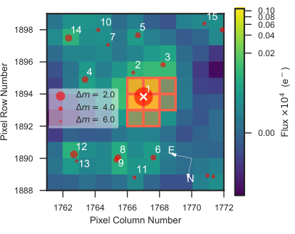
GJ 3473 (TIC 452866790) was observed by TESS with a two-minute cadence in Sector 7 (Camera #1, CCD #3) between 7 January and 2 February 2019 and is listed to have a transiting planet candidate on the TESS releases website (TOI–488.01). Due to its proximity to the ecliptic plane, it will not be observed again by TESS during its primary mission, but will be revisited in Sector 34 of the TESS extended mission in the third year33 3 https://heasarc.gsfc.nasa.gov/cgi-bin/tess/webtess/wtv.py?Entry=452866790, visited on 28 April 2020. The time series had a gap between and because of the data downlink and telescope re-pointing (see Fig. 2). The light curves produced by the Science Processing Operations Center (Jenkins et al. 2016, SPOC;) are available on the Mikulski Archive for Space Telescopes44 4 https://mast.stsci.edu. For our analysis, we used the systematics-corrected simple aperture photometry (PDC-SAP) light curve (Smith et al. 2012; Stumpe et al. 2012; Stumpe et al. 2014). A plot of the target pixel file (TPF) and the aperture mask that is used for the simple aperture photometry (SAP), generated with tpfplotter55 5 https://github.com/jlillo/tpfplotter, is shown in Fig. 1. The TESS data have a median internal uncertainty of (parts per thousand) and root mean square (rms) of around the mean. See Luque et al. 2019, Dreizler et al. 2020, Nowak et al. 2020, and Bluhm et al. 2020 for further details on the applied methodology.
2.2 High-resolution spectroscopy
High-resolution follow-up spectroscopy of the TESS planet candidates is arranged by the TESS follow-up programme (TFOP), ‘Precise Radial Velocities’ SG4 subgroup66 6 https://tess.mit.edu/followup/. The goal is to achieve a full validation of the candidates and to ultimately provide their mass measurement.
CARMENES.
As part of the CARMENES guaranteed time observation programme to search for exoplanets around M dwarfs (Reiners et al. 2018), we observed GJ 3473 with CARMENES (Quirrenbach et al. 2014, Calar Alto high-Resolution search for M dwarfs with Exoearths with Near-infrared and visible Echelle Spectrographs;). CARMENES is a high-resolution spectrograph at the Calar Alto telescope that consists of two cross-dispersed echelle channels operating in the spectral ranges of in the visible light (VIS, ) and in the near infrared (NIR, ), respectively. The observations began at the end of March 2019, just after the announcement of the transiting planet candidate, and ended in January 2020. In this period, we collected 67 pairs of VIS and NIR spectra with exposure times of about each. Within the standard CARMENES data flow, the spectra are calibrated using CARACAL (Caballero et al. 2016b), while the RVs are calculated using SERVAL (Zechmeister et al. 2018). The RVs are corrected for barycentric motion, secular perspective acceleration, as well as instrumental drift. To reconstruct small systematic radial-velocity variations, so called nightly zero-point offsets, we use the measured RVs of all other stars with only small intrinsic RV variations from the respective observing nights (see Trifonov et al. 2018; Tal-Or et al. 2019; Trifonov et al. 2020, for details). Spectra without simultaneous Fabry-Pérot drift measurements or a signal-to-noise ratio (S/N) lower than are excluded during the process, which results in a total of 64 RV measurements in the VIS and 66 in the NIR. The RVs show a median internal uncertainty of and a weighted rms (wrms) of in the VIS and and in the NIR, respectively. The high scatter in the NIR channel corresponds to our expectation from the photon-noise limit considering the median measured S/N of for the NIR observations (see Bauer et al. 2020, for a detailed analysis of the performance of CARMENES). Due to the low RV amplitude of the transiting planet candidate (), we therefore used only the VIS data for this study.
IRD.
In the course of the Subaru IRD TESS Intensive Follow-up Project (proposal S19A-069I), we observed GJ 3473 with the InfraRed Doppler spectrograph (Kotani et al. 2018, IRD;), a near-infrared, adaptive-optics (AO) corrected, high-resolution spectrograph (, ) installed on the Subaru 8.2 m telescope. The integration time was set to so that the extracted one-dimensional spectra have S/N ratios of per pixel at . A total of 56 frames were acquired for GJ 3473 by IRD on 12 different nights between April 2019 and December 2019, all of which had simultaneous reference spectra of the laser frequency comb. The reduction of the raw data was performed with the IRAF echelle package (Tody 1993), including the wavelength calibration using thorium-argon hollow cathode lamps. For the RV analyses, wavelengths were re-calibrated more precisely based on the laser frequency comb spectra. RVs were measured using the forward modelling technique described by Hirano et al. 2020, in which the time-variable telluric absorptions and the instantaneous instrumental profile of the spectrograph were modelled and taken into account in the RV fits. The IRD RVs show a median internal uncertainty of and a wrms of .
HARPS.
GJ 3473 was also observed by the High Accuracy Radial velocity Planet Searcher (Mayor et al. 2003, HARPS;) as part of the ESO programme 1102.C-0339(A). The spectrograph, installed at the ESO La Silla 3.6 m telescope, covers the spectral range from and has a resolution of . The observations presented here were taken between May 2019 and March 2020. Their exposure times ranged between . We use the reduced spectra from the HARPS Data Reduction Software (Lovis & Pepe 2007, DRS;) and compute their RVs following Astudillo-Defru et al. 2017b, which resulted in a lower rms scatter compared to the RVs retrieved with the SERVAL pipeline. They are calibrated for the barycentric motion, secular perspective acceleration, and instrumental drift. For the HARPS RVs, we obtain a median internal uncertainty of and a wrms of .
2.3 Ground-based transit follow-up
The TFOP subgroup SG1 provides seeing-limited photometry follow-up observations of the TESS planet candidates in order to supplement the available photometry and to provide improved ephemerides for the targets. An overview of the observations, the instruments and the filters used is given in Table 1.
| Telescope | Date | Transit ( a ) (a)(a) ( a ) (a)(a)footnotemark: | Filter | texp | Duration ( b ) (b)(b) ( b ) (b)(b)footnotemark: | Nobs | Aperture | rms |
|---|---|---|---|---|---|---|---|---|
| [] | [min] | [pix] | [ppt] | |||||
| LCOGT McD | 2019-03-19 | |||||||
| MuSCAT2 | 2019-12-21 | |||||||
| MuSCAT2 | 2019-12-21 | |||||||
| MuSCAT2 | 2020-01-02 | |||||||
| MuSCAT2 | 2020-01-02 | |||||||
| MuSCAT2 | 2020-01-02 | |||||||
| MuSCAT | 2020-01-18 | |||||||
| MuSCAT | 2020-01-18 | |||||||
| LCOGT CTIO | 2020-02-21 | |||||||
| LCOGT CTIO | 2020-02-27 | |||||||
| LCOGT SAAO | 2020-03-13 |
LCOGT.
We used four transit observations of GJ 3473 from the Las Cumbres Observatory global telescope network (Brown et al. 2013, LCOGT;). The observations were taken with the SINISTRO CCDs at the telescopes of the LCOGT, which have a pixel scale of and a field of view (FOV) of each. The first transit was observed from the McDonald Observatory (McD) on 19 March 2019 in the filter, two transits were observed from the Cerro Tololo Interamerican Observatory (CTIO) on 21 and 27 February 2020 in filter and one transit in filter on 13 March 2020 from South African Astronomical Observatory (SAAO). We calibrated the images with the standard LCOGT Banzai pipeline (McCully et al. 2018) and extracted the light curves using AstroImageJ (Collins et al. 2017).
MuSCAT.
GJ 3473 was observed on 18 January 2020 by the Multi-color Simultaneous Camera for studying Atmospheres of Transiting planets (Narita et al. 2015, MuSCAT;) mounted at the telescope at the Okayama Astro-Complex on Mt. Chikurinji, Japan. MuSCAT is a multi-colour instrument that performs imaging in the , and -filter bands at the same time. Each camera has a FOV of with a pixel scale of . Due to a large scatter in the band, we only use the and light curves here. The individual images are corrected for dark current and flat fields, and the light curves are generated using a custom pipeline that is described in Fukui et al. 2011.
MuSCAT2.
We made use of two transit observations from MuSCAT2 (Narita et al. 2019). The instrument is mounted at the Telescopio Carlos Sánchez at the Observatorio del Teide, Spain. MuSCAT2 operates simultaneously in the , , , and passbands and has a FOV of at resolution. One transit was observed on 21 December 2019, from which we use the observations in the and bands. The other transit was observed on 2 January 2020, from which we use the observations in the , and bands. Both transits were observed defocussed to optimise the quality of the photometry. The transit signal had too low S/N in the band to be useful in the fitting, and the band observations were affected by systematics on the night of 21 December. The photometry was produced using a dedicated MuSCAT2 photometry pipeline (see Parviainen et al. 2019, for details) and the detrended light curves were created by a fit that aims to simultaneously choose the best target and comparison star apertures, model the systematics using a linear term, and include the transit using PyTransit (Parviainen 2015).
USAFA.
We used the brand-new, recently commissioned 1 m USAFA Telescope, which is an optically-fast Ritchey-Chrétien telescope with a wide field of view 0.9 deg2 and an STA1600 CCD installed on the outskirts of Colorado Springs. We observed GJ 3473 on 04 March 2020. The USAFA data did not firmly detect the transit on target, but ruled out nearby eclipsing binaries in all other stars within the apertures of TESS, LCOGT, and MuSCAT/2 (Fig. 1).
2.4 Photometric monitoring
We used long-term photometric monitoring of GJ 3473 to search for periodic signals associated with the rotation period of the star.
TJO.
We observed GJ 3473 with the 80 cm Joan Oró telescope (TJO) at Observatori Astronòmic del Montsec, Spain. The star was monitored between 31 January and 8 May 2020 for a total of 32 nights. Our observations were performed in the Johnson filter by using the main imaging camera LAIA, which has a 4k 4k back illuminated CCD with a pixel scale of 0.4 arcsec and a FOV of 30 arcmin. We calibrated each image for bias and dark current as well as applied flat field images using the ICAT pipeline (Colome & Ribas 2006). Differential photometry was extracted with AstroImageJ using the aperture size and set of comparison stars that minimised the rms of the photometry. Low S/N data due to high airmass or bad weather were removed. The data were binned to one measurement per hour. The median internal uncertainty is , while the rms is around the mean. For the estimation of the stellar rotation period with a Gaussian process, we binned these data to one data point per night. This reduces short term variations caused by jitter and yields a median internal uncertainty of and a rms of around the mean.
MEarth.
The all-sky transit survey MEarth consists of 16 robotic telescopes with a FOV of located at two observatories in the southern and northern hemisphere (Berta et al. 2012). We use archival photometric monitoring data from the Mearth-North project DR888 8 https://www.cfa.harvard.edu/MEarth/DR8/ covering the time span from and . In total, we retrieved observations of GJ 3473 from the archive. They were observed with telescopes and in the broad RG715 filter. For the photometric analysis of the host star, we use the individual nightly binned time series, which shows a median internal uncertainty of and a rms of around the mean.
2.5 High-resolution imaging
As part of the standard process for validating transiting exoplanets and to assess the possible contamination of bound or unbound companions on the derived planetary radii (Ciardi et al. 2015), high-resolution images of GJ 3473 were taken within the TFOP ‘High Resolution Imaging’ SG3 subgroup.
Gemini/NIRI.
Nine images of GJ 3473 in the Br narrow filter ) were taken with the NIRI instrument mounted at the 8.1 m Gemini North telescope (Hodapp et al. 2003) on 22 March 2019 as part of the Gemini programme GN-2019A-LP-101. The science frames had an exposure time of each and were dithered in a grid pattern with spacing (). A sky background image was created by median combining the dithered images. The basic reduction included bad pixel interpolation, flatfield correction, sky background subtraction, and alignment and co-adding of the images.
Keck/NIRC2.
The Keck Observatory observations were made with the NIRC2 instrument on the 10.0 m Keck II telescope behind the natural guide star AO system (Service et al. 2016, and references therein). The observations were taken on 25 March 2019 in the standard three-point dither pattern that is used with NIRC2 to avoid the left lower quadrant of the detector, which is typically noisier than the other three quadrants. The dither pattern step size was and was repeated four times. The observations were also obtained in the narrow-band Br filter ) with an integration time of with one coadd per frame for a total of on target. The camera was in the narrow-angle mode with a full field of view of arcsec and a pixel scale of 0.099442 arcsec pix-1.
3 Properties of GJ 3473
| Parameter | Value | Ref. |
| Name and identifiers | ||
| Name | GJ 3473 | Gli91 |
| Alt. name | G 50–16 | Gic59 |
| Karmn | J08023+033 | Cab16 |
| TIC | 452866790 | Stas19 |
| TOI | 488 | TESS releases |
| Coordinates and spectral type | ||
| (J2000) | 08 02 22.88 | Gaia DR2 |
| (J2000) | +03 20 19.7 | Gaia DR2 |
| Sp. type | M4.0 V | Haw96 |
| [mag] | Gaia DR2 | |
| [mag] | Stas19 | |
| [mag] | 2MASS | |
| Parallax and kinematics | ||
| [] | Gaia DR2 | |
| [] | Gaia DR2 | |
| [] | Gaia DR2 | |
| [] | Gaia DR2 | |
| [] | This work | |
| [] | This work | |
| [] | This work | |
| [] | This work | |
| Photospheric parameters | ||
| [K] | This work | |
| [dex] | This work | |
| [dex] | This work | |
| Physical parameters | ||
| [] | This work | |
| [] | This work | |
| [] | This work | |
| Activity parameters | ||
| pEW (H) [] | This work | |
| [dex] | This work | |
| [] | This work | |
| [d] | This work | |
The star GJ~3473 (G 50–16, Karmn J08023+033) was included in the TESS Input Catalogue as TIC 452866790 and declared a TESS Object of Interest (TOI) after the transiting planet candidate was found. A summary of the stellar parameters is given in Table 2. The star was classified as an M4.0 V star by Hawley et al. 1996, but it was never subject to an in-depth analysis of its properties (Newton et al. 2014, e.g.). To determine precise stellar parameters, we used the high-resolution spectra from the CARMENES follow-up observations. Following Passegger et al. 2018; Passegger et al. 2019 and applying a measured upper limit of , we calculated the effective temperature , , and from a fit to a grid of PHOENIX stellar atmosphere models (Husser et al. 2013) using a method. The derived matches the literature spectral type taking into account the uncertainties in both parameters (Alonso-Floriano et al. 2015; Passegger et al. 2018; Cifuentes et al. 2020). Next, we determined the bolometric luminosity, , by integrating the spectral energy distribution in 14 broad passbands from optical to with the Gaia DR2 parallax (Gaia Collaboration et al. 2018) as in Cifuentes et al. 2020. The radius, , was subsequently calculated using the Stephan-Boltzmann law. Lastly, the mass, , was derived from the Schweitzer et al. 2019 empirical mass-radius relation derived from eclipsing binaries. The values determined in this way are consistent with the mass and radius determined from isochrones (Morton 2015). We updated the Galactocentric space velocities according to Cortés-Contreras 2016 by combining the Gaia DR2 parameters and the absolute velocity measured from the cross-correlation function (CCF) of the spectra with a weighted binary mask (Lafarga et al. 2020). Using the space velocities and the BANYAN Bayesian classification tool, we found no indication that GJ 3473 is a member of any nearby young stellar association. Instead, it is most probably a field star located in the Galactic thin disk (Gagné et al. 2018).
GJ 3473 is listed in the Washington Double Star catalogue (Mason et al. 2001) as the primary of the binary system LDS 5160 (Luyten Double Star), with a date of first satisfactory observation in 1949. The secondary, at an angular separation of 49.290.09 arcsec to the southeast of GJ 3473 ( = 222.814.1 deg), is LP~544–12 (GJ 3474, source #3 in Fig. 1), a = 12.2 mag M6 V star that shares the proper motion and parallax values of our planet-host star, but with a third of its mass (Luyten 1979; Reid et al. 1995; Newton et al. 2017). At the distance of GJ 3473, the angular separation between the two stars translates into a projected physical separation of 1349.93.1 au.
4 Analysis and results
4.1 Transit search within the TESS light curve

A transiting planet candidate around GJ 3473 was announced on 14 March 2020 via the TESS releases website1010 10 https://tess.mit.edu/toi-releases. The candidate passed all tests from the SPOC Data Validation Report (Twicken et al. 2018; Jenkins 2002; Li et al. 2019) and it is listed on the Exoplanet Follow-up Observing Program (ExoFOP)1111 11 https://exofop.ipac.caltech.edu/tess/target.php?id=452866790 webpage as having a period of and a transit depth of . We performed an independent transit search on the PDC-SAP light curve using the Transit-Least-Squares method (Hippke & Heller 2019, TLS;)1212 12 https://github.com/hippke/tls. We consider a signal to be significant if it reaches a signal detection efficiency (Alcock et al. 2000; Pope et al. 2016, SDE;) of at least . The TLS shows a highly significant transit signal () with an SDE of and a transit depth of . After pre-whitening of the photometric data by fitting for this signal, a TLS of the residuals shows no remaining significant signals with .
4.2 Adaptive-optics imaging and limits of photometric contamination


As part of our standard process for validating transiting exoplanets and to assess the possible contamination of bound or unbound companions on the derived planetary radii (Ciardi et al. 2015), we investigated the deep AO images from NIRC2 at Keck II and NIRI at Gemini North shown in Fig. 3. Both images were taken in Br narrow filters. No companions are visible to a separation of . The contrast curves are obtained by injecting fake sources of different brightness at different separations from the star and determining the radial detection limit. The NIRC2 observations are sensitive up to a contrast of at a separation of to the star, but only span the region of the inner . The area further out up to is covered by the NIRI image, which reaches a contrast level of . We therefore conclude, based on a combination of the contrast curves, a visual inspection of the AO images in Fig. 3, and the Baraffe et al. 2003 COND models for an approximate solar age, that GJ 3473 does not have a high-mass brown dwarf or more massive companion at 13–160 au. Furthermore, using additional 2MASS imaging and Gaia DR2 astro-photometry, we ruled out the presence of stellar companions of any mass at separations beyond 160 au up to a few thousands au (excluding the known companion LP 544–12). Another indicator for binarity is the re-normalised a posteriori mean error of unit weight (RUWE), which quantifies the goodness-of-fit of the astrometric solution in the Gaia DR2 (Arenou et al. 2018; Lindegren et al. 2018). At approximate separations between 1.3 au and 13 au, any hypothetical stellar companion would cause GJ 3473 to have a Gaia RUWE value larger than 1.41 (its actual value is 1.06; Cifuentes et al. 2020, and references therein) and an asymmetric point spread function in the NIRC2 and NIRI images. At separations closer than 1.3 au, we would see a double-peaked CCF or a long-term trend in the CARMENES RV data. We cannot exclude, however, the presence of substellar objects of a few Jupiter masses at wide separations (with orbital periods much longer than the RV coverage) or unfavourably aligned objects at close separations.
Additionally, we assessed the photometric contamination of the TESS light curves using Eq. 6 from Espinoza et al. 2019b. From the AO images, we obtained upper limits from in contrast for the inner area from , which correspond to contamination below . For the nearby Gaia sources apparent in Fig. 1, we make use of the fact that the TESS and Gaia -band filter are very similar. We find that for the brightest nearby source (# 3 in Fig. 1), which is its binary companion LP 544–12, the dilution factor would be 0.96. However, given the separation of to GJ 3473, this is negligible and, thus, we assume for our modelling that there are no contaminating sources nearby.
4.3 Transits only modelling
In order to refine the orbital period of the transiting planet candidate that was determined from the TLS analysis and to evaluate whether the individual follow-up observations show adequate transit detections, we first investigated the photometric observations separately from the RV measurements.
For all modelling tasks in this work, we used juliet1313 13 https://juliet.readthedocs.io/en/latest/ (Espinoza et al. 2019b), a fitting tool that uses nested sampling to efficiently evaluate the parameter space of a given prior volume and to allow for model comparison based on Bayesian evidences. Here, juliet combines publicly available packages for RVs and transits, namely, radvel1414 14 https://radvel.readthedocs.io/en/latest (Fulton et al. 2018) and batman1515 15 https://www.cfa.harvard.edu/~lkreidberg/batman/ (Kreidberg 2015). It allows us to choose among a range of different nested sampling algorithms for the fitting. We opted for dynesty1616 16 https://github.com/joshspeagle/dynesty (Speagle 2020) because of its simple usage with regard to multi-processing. Additionally, juliet provides the implementation of Gaussian processes in the models using either george1717 17 https://george.readthedocs.io/en/latest/ (Ambikasaran et al. 2015) or celerite1818 18 https://celerite.readthedocs.io/en/stable (Foreman-Mackey et al. 2017).
As a first step, we modelled all of the available ground based follow-up observations of transit events obtained by the TFOP SG11919 19 As of 13 March 2020 separately with the TESS light curve while fitting for the transit centre of each transit (see Eastman et al. 2019, and the documentation of juliet for details of the implementation). In doing so, we re-parametrised the scaled semi-major axis to the stellar density, . In this manner we can make use of the derived stellar parameters to obtain a density estimation as a fit prior. Furthermore, we implement the parameter transformation suggested by Espinoza 2018 and fit for the parameters, and instead of the planet-to-star radius ratio, , and the impact parameter, . A quadratic limb-darkening model is used for the TESS data (Espinoza & Jordán 2015), which is parametrised by the and parameters (Kipping 2013), while a linear model is used for the ground-based follow-up observations. We used a linear term to detrend the LCOGT and MuSCAT light curves with airmass, while the MuSCAT2 light curves were pre-detrended (see Sect. 2.3). Based on the results from Sect. 4.2, we fix the dilution factor to one for all instruments, but consider free individual instrumental offsets. Also instrumental jitter terms are taken into account and added in quadrature to the nominal instrumental errorbar.
By carrying out this pre-analysis, we were able to disregard observations that show no, or only marginal transits, or seem to be only apparent transits with transit centres far from a linear ephemeris. The final dataset, which is presented in Sect. 2 and which we use for the analysis in this work, includes transit events with observations of firm transit detections (cf. Table 1).
In the next step, we combine these observations and then fit for a common period and time of transit centre that serve as a basis for the joint analysis. In doing so, we determine d and .
4.4 RV only modelling
We approach the analysis of the RVs with a signal search in the data, proceeding as if we do not know of the transiting planet a priori. In Fig. 4, the generalised Lomb-Scargle periodograms (Zechmeister & Kürster 2009, GLS;) of the residuals from different fits of increasing complexity to the combined RVs from CARMENES, IRD, and HARPS are shown. We normalised the periodograms using the parametrisation of Zechmeister & Kürster 2009. For all fits, we used Gaussian distributed priors for the signal of the transiting planet candidate based on the results from Sect. 4.3 and a narrow uniform range around the peak of the second signal. Instrumental offsets and jitter are treated separately for each dataset. For comparison, we list the Bayesian evidences of the fits in Table 4.
The first panel in Fig. 4 shows the periodogram of the residuals after fitting a flat model that only includes offsets and instrumental jitter to the CARMENES, IRD, and HARPS measurements. The strongest signal apparent in the RV data is a period at . After subtracting this periodicity with a circular Keplerian fit, the residual periodogram shows a significant signal (), coincident with the period of the transiting planet at (see the middle panel of Fig. 4). The FAP for a signal to occur especially at this frequency can be evaluated using the method by Baluev 2008 and the power of the signal in a Lomb-Scargle periodogram. By this means, we find a spectral . We verify this using a bootstrap method of random realisations over a decreasing frequency range centred on the period in question, which yields . This is in agreement with the Baluev method and we therefore assume a FAP of for the signal to occur at the expected period. Furthermore, the phase of this signal matches the phase of the planet candidate from TESS and we thus report a highly significant detection of the transiting planet candidate in the RV. The two other signals of significant power at periods of and are aliases of the former signal of the transiting planet due to the approximately daily sampling. This is reflected by the fact that they disappear when the signal is fitted together with the period of the transiting planet at (see the bottom panel of Fig. 4). Given that RV data provide more information on the eccentricity of an orbit, we performed an analogous analysis using eccentric orbits. We find that the difference between a circular and eccentric orbit is indistinguishable () and, therefore, we use the results for the simpler circular model fits. The residuals of this fit comprising two circular Keplerian signals do not show any further periodicities with FAPs above our significance criterion of .
4.5 Joint modelling

For the final retrieval of the most precise parameters we perform a joint fit of the TESS observations, the ground-based transit follow-ups, and the combined RV data. The model includes two circular planets: firstly, the transiting planet that is detected in the photometry and RV data and; secondly, a non-transiting planet that is only apparent in the RV data. The model of the joint fit comprises 58 free parameters, which turns the fit into a high-dimensional problem. A fit with uninformed priors would therefore be very costly. Hence, we make use of the findings from the photometry-only analysis in Sect. 4.3 and the RV-only analysis in Sect. 4.4 – that is, we implement Gaussian distributed priors for the planetary parameters, as, for example, in Brahm et al. 2019; Espinoza et al. 2019a; Kossakowski et al. 2019; Luque et al. 2019; or Bluhm et al. 2020. Since we use uninformed priors for the planetary parameters for the transit and RV-only fits, nested sampling warrants an efficient exploration of the possible parameter space fitting the individual datasets. Planetary parameters specific to a given data type, such as the planetary semi-amplitude in RV data or planet-to-star radius (and others) in transit data, would not change significantly in a joint fit as they are independent from the other data to first order. Generally, this also holds true for the shared parameters since they are mostly driven by either one or the other method. Likewise, using the posterior results from the transit-only and RV-only fits as a prior knowledge for the joint fit is therefore justified given that the chosen prior volume for the joint fit does not restrict the posterior volume from the individual fits. Following this, the width of the priors that we choose for the planetary parameters of the joint fit are three times the standard deviation of the posterior results from the individual best fits. It limits the computational cost, but still allows the nested sampling algorithm to freely explore the parameter space since the Gaussian distribution has no strict borders. In the end, the posterior distribution of our joint fit is much narrower than that of the input priors, which shows that the input priors were conservatively chosen to map the relevant parameter space and did not reject crucial possible solutions. Descriptions and justifications of the adopted instrumental parameters and priors can be found in the respective subsections, Sect. 4.3 and Sect. 4.4. A summary of the used priors is given in Table 7.
In Fig. 6 and Fig. 5, we show the final models of the joint fit based on the posterior of the sampling. The median posteriors of the planetary parameters are shown in Table 3 and the full list of the posteriors of the instrumental parameters is given in Table 9.
| Parameter | Posterior ( a ) (a)(a) ( a ) (a)(a)footnotemark: | Units |
|---|---|---|
| Stellar parameters | ||
| Planetary parameters | ||
| d | ||
| d | ||
| … | ||
| … | ||
| (fixed) | … | |
| (fixed) | … | |
| d | ||
| d | ||
| (fixed) | … | |
| (fixed) | … | |
4.6 Stellar activity
We investigated a set of activity indicators derived from the CARMENES spectra to search for signals of stellar activity that would interfere with the transiting planet candidate or provide information on the origin of the second periodicity that is visible in the RV data (see Sect. 4.4). In Fig. 7, the GLS periodograms of 13 selected activity indicators, as well as our applied nightly zero-point offsets, are shown. The chromatic index (CRX) and the differential line width (dLW) are products of the SERVAL reduction pipeline (Zechmeister et al. 2018). From the CCF (see Sect. 3), the full-width at half-maximum (FWHM), the contrast, and the bisector span are determined (Lafarga et al. 2020). The pseudo-equivalent width after subtraction of an inactive template spectrum (pEW′) of the chromospheric H, Ca ii IRT (a, b and c), He i and He i D3 lines, and the photospheric TiO and TiO indices are calculated following Schöfer et al. 2019.
A measured median pEW of the H line of indicates that GJ 3473 is a rather inactive star (Jeffers et al. 2018). We find a significant, although moderate, correlation between RV and the CRX and Na i D activity indices, however, the GLS periodograms from the extensive set of activity indicators do not show any power at the frequencies of the transiting planet candidate or the signal. The dLW, CCF contrast, TiO , and He i show a forest of signals with in the range of approximately . This is consistent with a lower limit of the stellar rotation period to be longer than as determined from , however, there is no common periodicity or conclusive pattern, which would hint at the rotation period of the star. The most significant signal, which is apparent in the He i indicator, has a period of around . From the HARPS spectra we derive , which is equivalent to a stellar rotation period of following the vs. relationship of Astudillo-Defru et al. 2017a. We also investigated GLS periodograms of the HARPS activity indicators derived by the DRS pipeline, but we do not find any significant periodicity and, therefore, we do not present them here.
4.7 Photometric stellar rotational period
We combined the -band TJO data collected between January and May 2020 and the RG715-band MEarth data taken between 2008 and 2018 to determine a stellar rotation period. A marginalised likelihood periodogram (Feng et al. 2017, MLP;) analysis of the combined data, where we fit for jitter and offsets between the datasets, indicated a preliminary periodicity of 160 d. The MLP uses sinusoidal functions to model possible significant signals. However, stellar activity tends to be quasi-periodic and can also deviate significantly from a simple sinusoidal. Thus, we used a Gaussian process (GP) to fit the photometry in a second approach.
We used juliet and select the quasi-periodic kernel by george for the modelling of the photometric data:
| (1) |
where is the amplitude of the GP component given in (or when applied to RV data), is the amplitude of GP sine-squared component, is the inverse length-scale of the GP exponential component given in , is the period of the GP quasi-periodic component given in days, and is the temporal distance between two measurements. To perform a blind search for quasi-periodic signals with the GP model, we put in uninformed priors for , and , but take a uniform range from for .
In doing so, the data of each instrument are averaged into nightly bins because of the large dataset and the computationally expensive log-likelihood evaluation of the used kernel. A daily sampling of the photometry is reasonable since we are searching for signals with periods of at least multiple days (see Sect. 4.6). Furthermore, binning reduces short-term variations due to jitter and decreases the uncertainties of the data points. For the GP model, we consider that each dataset can have different solutions for the amplitude parameters, and . This accounts for the possibility that the stellar activity depends on wavelength and might impact each instrument differently. However, the timescale parameters, such as the rotational period, , and the exponential decay of the signal , for example, due to spot-life time, should not depend on the instrument. For the latter two parameters, we therefore allow only for global solutions of the GP model. We also model the flux offset between the photometric datasets, as well as an extra jitter component, which is added in quadrature to the diagonal of the resulting covariance matrix. Our GP fit, using unconstrained priors (Table 8), results in only one specific region within the prior volume that has a high density of posterior samples with high likelihood. We show the nightly binned photometric data and the GP fit with its uncertainties in Fig 8.
From the posterior solutions we derive a photometric rotation period, d for GJ 3473, which is consistent with the result from the MLP analysis and, within , with the expected period from . Both estimates show that GJ 3473 is a slow rotator, which should not exhibit strong signals related to activity. This is also in agreement with the spectroscopic activity indicators, which do not exhibit a predominant periodicity and no H activity.
4.8 Investigation of the signal


| Model | Periods ( a ) (a)(a) ( a ) (a)(a)footnotemark: | ||
| [] | |||
| 0 Planets | … | ||
| 1 Planet | |||
| 1 Planet | |||
| 1 Planet + GP | |||
| 2 Planets | 15.5, 1.20 |
The signal seems to be unrelated to stellar activity or the stellar rotation period. Following Fig. 5, the signal looks stable for the entire period of observations and shows no significant deviations from a circular Keplerian motion. However, we thoroughly examined the signal in order to asses its nature and to test whether we can attribute it unambigously to a planetary origin.
We used juliet to perform a model comparison based on the Bayesian evidence of different models, applied to the RV data only, in order to check whether the signal is indeed best fit with a Keplerian model. The log-evidences of the results are shown in Table 4. As outlined by Trotta 2008, we consider a difference of as weak evidence that one of the models is preferred over the others and that a model is significantly favoured. We use Gaussian distributed priors based on the posterior solutions from Sect. 4.3 to account for the transiting planet candidate, and uniform priors for instrumental offsets and jitter. However, we adopted two approaches to include the signal in the modelling: on the one hand, a simple two-planet model is fitted to the data and on the other hand, we implement a quasi-periodic GP (see Eq. 1 in Sect. 4.7) to test the possibility that the second signal does not have a Keplerian nature and is only of a quasi-periodic origin, for example, due to stellar activity. We find a difference of () in favour of the two-planet model compared to the model, including a quasi-periodic component for the signal. This offers only weak evidence, confirming, nonetheless, that the signal is legitimately fitted by a Keplerian model.
Another way to test the coherence of a signal for a given dataset is the use of the so-called stacked Bayesian generalised Lomb-Scargle periodogram (Mortier et al. 2015, s-BGLS;). The diagram in the left panel of Fig. 9 shows the probability of the signal normalised to the minimum of the considered frequency range (Mortier & Collier Cameron 2017) for an increasing number of observations. The period of the signal is uncertain when only a few observations are included, but starting with more than 80 observations, a signal of consistently rising probability is detected at the period in question. This indicates that the signal is stable in phase and amplitude over the whole observational period of a time baseline, as is likely for a planetary signal. A colour-coded bar on the right side of the diagram specifies which of the instruments the considered data points originate from. As there are no variations of the signal caused by chunks of data from one specific instrument, we can also conclude that the signal is consistent between the different instruments.
Even though there are no obvious signs of more than one transiting planet in the TESS light curve (see Sect. 4.1), we searched for transits of the signal based on its parameters derived from the RV observations. Since the period of the planet is larger than half of the time span of the TESS data, which comprise only one sector, a potential transit is likely to occur only once in the data. The right panel in Fig. 9 shows the TESS data phase-folded to the expected time of transit centre. No obvious transit signals are visible. However, to quantify whether in fact there is no transit signal, we ran two more juliet fits on the TESS data using Gaussian distributed priors based on the posterior of the planetary parameters in Table 3. The model considering only the transiting planet is favoured by over the model that treats the second periodicity as a transiting planet. Thus, we conclude that no significant transiting signal is associated with the periodicity.
5 Discussion
5.1 GJ 3473 b
| Parameter | Posterior ( a ) (a)(a) ( a ) (a)(a)footnotemark: | Units | |
| GJ 3473 b | GJ 3473 c | ||
| Derived transit parameters | |||
| … | … | ||
| … | … | ||
| … | … | ||
| … | deg | ||
| ( d ) (d)(d) ( d ) (d)(d)footnotemark: | … | … | |
| … | … | ||
| … | h | ||
| Derived physical parameters ( b ) (b)(b) ( b ) (b)(b)footnotemark: | |||
| … | |||
| … | |||
| … | |||
| ( c ) (c)({c}) ( c ) (c)({c})footnotemark: | |||
| ESM ( d ) (d)(d) ( d ) (d)(d)footnotemark: | … | … | |
Our derived mass and radius confirm the planetary nature of the transiting planet candidate detected by TESS. GJ 3473 b has a mass of and a radius of , which correspond to a density of and, thus, fits in the regime of Earth-sized planets with a density consistent with a composition dominated by MgSiO3 (see Fig. 10). A summary of the derived physical parameters of the planet can be found in Table 5.
With an insolation flux of , GJ 3473 b is one of the hottest transiting Earth-mass planets with a dynamical mass measurement that has been detected so far (see Fig. 11). Its equilibrium temperature corresponds to , assuming a zero Bond albedo. If the planet had an atmosphere, thermochemical equilibrium calculations predict water and methane to be the dominant opacity sources in the near/mid infrared (NIR/MIR) of the transmission spectrum of GJ 3473 b, assuming a cloud-free solar-abundance scenario (Madhusudhan 2012; Mollière et al. 2015; Molaverdikhani et al. 2019b, e.g.); see the red line in Fig. 12. In this scenario, the main transmission spectral features in the optical are expected to be alkali (Na and K), although their expected strength depends on a number of parameters such as the planetary atmospheric metallicity. The emission spectrum is heavily muted by water and methane absorption, causing very low relative flux at wavelengths shorter than 3 m; see the blue line in Fig. 12. The dominant spectral features of a cloudy atmosphere in the optical and NIR are expected to be similar to those of a cloud-free atmosphere, although with lower amplitudes and less pronounced methane features (Molaverdikhani et al. 2020).
In addition, disequilibrium processes could change the composition and thermal structure of the planetary atmosphere. Depending on the exact temperature structure and methane abundance profile, vertical mixing could lead to methane quenching (Molaverdikhani et al. 2019a, e.g.). Hydrocarbon haze (soot) production could act as a carbon-sink in the atmosphere, which might cause a reduced carbon-to-oxygen (C/O) ratio (Molaverdikhani et al. 2019a; Gao et al. 2020, e.g.). While haze opacities tend to obscure the optical to NIR wavelength range, a reduced C/O ratio could result in an enhancement of CO2 production. This causes a prominent feature at around (Kawashima & Ikoma 2019; Nowak et al. 2020, see e.g.). Atmospheres with higher metallicities are likely to lead to more prominent CO2 features (Heng & Lyons 2016; Molaverdikhani et al. 2019a; Nowak et al. 2020; Schlecker et al. 2020, see e.g.). Hence, this spectral feature appears to be a key feature to retrieve planetary atmosphere metallicities, which, in turn, helps us to understand the formation history of the planet and the stellar system.
The amplitudes of the transmission spectral features of GJ 3473 b are estimated to be around for the discussed model. This poses a challenge for future observations of this planet through transmission spectroscopy. However, the relatively high temperature of this planet causes the emission spectral features at wavelengths longer than 3 m to vary from tens of ppm in NIR to hundreds ppm in MIR wavelengths up to . We calculate the emission spectroscopy metric (ESM), based on Kempton et al. 2018, to be , which is close to what Kempton et al. 2018 classify as high-quality atmospheric characterisation targets ().
5.2 GJ 3473 c
Our RV modelling shows evidence for a second planet in the system. Its derived period is likely not linked to the stellar rotation period of as determined in Sect. 4.7. Furthermore, the analysis of a comprehensive set of activity indicators exhibits no signs of stellar activity at the period in question. The analysis of the pEW of the H line and the index describes GJ 3473 as a rather inactive star, which would contradict the relatively high RV amplitude of if the signal was attributed to activity (cf. Sect. 4.6). Furthermore, the signal is coherent for at least one year of observations and invariant with respect to the different instruments (see Sect. 4.8).
We therefore conclude that the signal in the RVs is caused by a second planet in the system, GJ 3473 c. The planet has a lower mass limit of . Further physical parameters derived for this planet are shown in Table 5. No transit signals of GJ 3473 c are found within the TESS data. An estimate of its bulk composition from theoretical models is not feasible because the derived mass places the planet just in the regime of the radius dichotomy between super-Earths and mini-Neptunes (Owen & Wu 2013; Jin et al. 2014; Fulton et al. 2017; Zeng et al. 2017; Cloutier & Menou 2020, e.g. ). However, the non-detection of transits is not unexpected when an orbit co-planar to GJ 3473 b () is assumed. The minimum inclination for at least grazing transits at a separation of from the host star would be considering a planet at the empirical upper radius limit for mini-Neptunes. At a distance of from the host star, GJ 3473 c receives times the stellar flux compared to Earth, which places it outside the inner boundary of the optimistic habitable zone, , as defined by Kopparapu et al. 2014. The planet therefore is a temperate super-Earth or mini-Neptune such as GJ~887~c (Jeffers et al. 2020), GJ~686~b (Lalitha et al. 2019; Affer et al. 2019), GJ~685 (Pinamonti et al. 2019) or GJ~581~c (Udry et al. 2007) (see Fig. 11).
5.3 Comparison to synthetic planet populations
We compare the planetary system of GJ 3473 with a synthetic M dwarf planet population from a core accretion model of planet formation (Burn et al. in prep.) to assess the frequency of such a configuration. There, planets like GJ 3473 b are relatively abundant and often accompanied by multiple other planets in the system. More than of their synthetic systems contain systems with a combination of planets similar to GJ 3473 b and c with respect to their masses and periods. The systems with an architecture closest to GJ 3473 suggest a low bulk density for the outer planet, which can currently not be tested observationally. Another theoretical prediction from the core accretion paradigm is a higher frequency of distant companions for volatile-poor inner planets such as GJ 3473 b (Schlecker et al. 2020). While the current results do not demonstrate any clear evidence for planets beyond GJ 3473 c, further long-term monitoring is needed to probe the outer system.
5.4 Search for transit timing variations
The period ratio of the two planets (, ) does not suggest the presence of strong transit timing variations (TTV) for the transiting planet. However, we used juliet to perform a fit that only explores possible TTVs in the system. For this, we re-ran the joint fit but fixed all parameters to the results in Table 3 and Table 9 and added a TTV parameter for each transit (Gaussian distributed prior with mean and a standard deviation of , see the documentation of juliet for details). Although the results in Fig. 13 indicate TTVs up to , the error bars are rather large. The main reason for this is the small transit depth of GJ 3473 b compared to the scatter of the data points (see Fig. 6). A GLS analysis of the TTVs reveals no significant periodicity that would indicate the presence of another massive planet in the system.
6 Conclusions
Here, we report the discovery of a planetary system around the M4.0 V dwarf GJ 3473 based on an extensive set of RV measurements from CARMENES, IRD, and HARPS, as well as space-based TESS photometry and photometric transit follow-up observations from LCOGT, MuSCAT, and MuSCAT2, and high-resolution images from Keck/NIRC2 and Gemini/NIRI. We confirm the planetary nature of GJ 3473 b (TOI-488.01) and present its detailed characterisation from a simultaneous fit of the RV and transit data. The short-period planet has a mass of and a radius of , which yields a density that is consistent with a rocky composition. The planet complements the sample of small planets with mass and radius measurements better than and contributes to the TESS mission’s primary goal to measure the masses of planets with radii smaller than . Its proximity to the host star makes GJ 3473 b attractive for thermal emission spectroscopy. Synthetic cloud-free emission spectra predict amplitudes of the transmission spectral features up to 100s ppm in the MIR.
The RV data show evidence for an additional, non-transiting planet in the system. GJ 3473 c has a minimum mass of and an orbital period of , which places it just outside the inner boundary of the habitable zone.
The planetary system of GJ 3473 is another multi-planet system discovered around an M dwarf with planets in the range of Earth-like masses to super-Earths and mini-Neptunes. A comparison with synthetic planet populations shows that systems similar to GJ 3473 may be relatively abundant and often host multiple planets. We therefore encourage further long-time monitoring of the system to find additional planets.
Acknowledgements.
CARMENES is an instrument at the Centro Astronómico Hispano-Alemán de Calar Alto (CAHA, Almería, Spain). CARMENES was funded by the German Max-Planck-Gesellschaft (MPG), the Spanish Consejo Superior de Investigaciones Científicas (CSIC), the European Union through FEDER/ERF FICTS-2011-02 funds, and the members of the CARMENES Consortium (Max-Planck-Institut für Astronomie, Instituto de Astrofísica de Andalucía, Landessternwarte Königstuhl, Institut de Ciències de l’Espai, Insitut für Astrophysik Göttingen, Universidad Complutense de Madrid, Thüringer Landessternwarte Tautenburg, Instituto de Astrofísica de Canarias, Hamburger Sternwarte, Centro de Astrobiología and Centro Astronómico Hispano-Alemán), with additional contributions by the Spanish Ministry of Economy, the German Science Foundation through the Major Research Instrumentation Programme and Deutsche Forschungsgemeinschaft (DFG) Research Unit FOR2544 “Blue Planets around Red Stars”, the Klaus Tschira Stiftung, the states of Baden-Württemberg and Niedersachsen, and by the Junta de Andalucía. Part of this work was funded by the the Ministerio de Ciencia e Innovación via projects PID2019-109522GB-C51/2/3/4 and AYA2016-79425-C3-1/2/3-P, (MEXT/)JSPS KAKENHI via grants 15H02063, JP17H04574, 18H05442, JP18H01265, JP18H05439, 19J11805, JP19K14783, and 22000005, JST PRESTO via grant JPMJPR1775, FCT/MCTES through national funds (PIDDAC, PTDC/FIS-AST/32113/2017) via grant UID/FIS/04434/2019, FEDER - Fundo Europeu de Desenvolvimento Regional through COMPETE2020 - Programa Operacional Competitividade e Internacionalização (POCI-01-0145-FEDER-032113), the FONDECYT project 3180063, Fundação para a Ciência e a Tecnologia through national funds and by FEDER through COMPETE2020 - Programa Operacional Competitividade e Internacionalização by these grants: UID/FIS/04434/2019; UIDB/04434/2020; UIDP/04434/2020; PTDC/FIS-AST/32113/2017 & POCI-01-0145-FEDER-032113; PTDC/FIS-AST/28953/2017 & POCI-01-0145-FEDER-028953. and the International Graduate Program for Excellence in Earth-Space Science. Part of the data analysis was carried out on the Multi-wavelength Data Analysis System operated by the Astronomy Data Center, National Astronomical Observatory of Japan. Funding for the TESS mission is provided by NASA’s Science Mission directorate. We acknowledge the use of public TESS Alert data from pipelines at the TESS Science Office and at the TESS Science Processing Operations Center. This research has made use of the Exoplanet Follow-up Observation Program website, which is operated by the California Institute of Technology, under contract with the National Aeronautics and Space Administration under the Exoplanet Exploration Program. Resources supporting this work were provided by the NASA High-End Computing Program through the NASA Advanced Supercomputing Division at Ames Research Center for the production of the SPOC data products. This paper includes data collected by the TESS mission, which are publicly available from the Mikulski Archive for Space Telescopes. This work makes use of observations from the LCOGT network. The analysis of this work has made use of a wide variety of public available software packages that are not referenced in the manuscript: Exo-Striker (Trifonov 2019), astropy Astropy Collaboration et al. 2018, scipy (Virtanen et al. 2020), numpy (Oliphant 2006), matplotlib (Hunter 2007), tqdm (da Costa-Luis 2019), pandas (The pandas development team 2020), seaborn (Waskom et al. 2020), lightkurve (Lightkurve Collaboration et al. 2018) and PyFITS (Barrett et al. 2012).References
- Affer et al. (2019) Affer, L., Damasso, M., Micela, G., et al. 2019, A&A, 622, A193
- Alcock et al. (2000) Alcock, C., Allsman, R., Alves, D. R., et al. 2000, ApJ, 542, 257
- Almenara et al. (2018) Almenara, J. M., DDorn, C., Bonfils, X., & Udry, S. 2018, MNRAS, 478, 460
- Alonso-Floriano et al. (2015) Alonso-Floriano, F. J., Morales, J. C., Caballero, J. A., et al. 2015, A&A, 577, A128
- Ambikasaran et al. (2015) Ambikasaran, S., Foreman-Mackey, D., Greengard, L., Hogg, D. W., & O’Neil, M. 2015, IEEE transactions on pattern analysis and machine intelligence, 38, 252
- Anglada-Escudé et al. (2013) Anglada-Escudé, G., Tuomi, M., Gerlach, E., et al. 2013, A&A, 556, A126
- Arenou et al. (2018) Arenou, F., Luri, X., Babusiaux, C., et al. 2018, A&A, 616, A17
- Astropy Collaboration et al. (2018) Astropy Collaboration, Price-Whelan, A. M., Sipocz, B. M., et al. 2018, AJ, 156, 123
- Astudillo-Defru et al. (2020) Astudillo-Defru, N., Cloutier, R., Wang, S. X., et al. 2020, A&A, 636, A58
- Astudillo-Defru et al. (2017a) Astudillo-Defru, N., Delfosse, X., Bonfils, X., et al. 2017a, A&A, 600, A13
- Astudillo-Defru et al. (2017b) Astudillo-Defru, N., Forveille, T., Bonfils, X., et al. 2017b, A&A, 602, A88
- Baluev (2008) Baluev, R. V. 2008, MNRAS, 385, 1279
- Baraffe et al. (2003) Baraffe, I., Chabrier, G., Barman, T. S., Allard, F., & Hauschildt, P. H. 2003, A&A, 402, 701
- Barrett et al. (2012) Barrett, P., Hsu, J. C., Hanley, C., et al. 2012, PyFITS: Python FITS Module
- Batalha et al. (2018) Batalha, N. E., Lewis, N. K., Line, M. R., Valenti, J., & Stevenson, K. 2018, ApJ, 856, L34
- Bauer et al. (2020) Bauer, F. F., Zechmeister, M., Kaminski, A., et al. 2020, A&A, 640, A50
- Berta et al. (2012) Berta, Z. K., Irwin, J., Charbonneau, D., Burke, C. J., & Falco, E. E. 2012, AJ, 144, 145
- Berta-Thompson et al. (2015) Berta-Thompson, Z. K., Irwin, J., Charbonneau, D., et al. 2015, Nature, 527, 204
- Bitsch et al. (2019) Bitsch, B., Raymond, S. N., & Izidoro, A. 2019, A&A, 624, A109
- Bluhm et al. (2020) Bluhm, P., Luque, R., Espinoza, N., et al. 2020, A&A, submitted
- Bonfils et al. (2018) Bonfils, X., Almenara, J.-M., Cloutier, R., et al. 2018, A&A, 618, A142
- Bonfils et al. (2013) Bonfils, X., Delfosse, X., Udry, S., et al. 2013, A&A, 549, A109
- Borucki (2016) Borucki, W. J. 2016, Reports on progress in physics. Physical Society (Great Britain), 79, 036901
- Borucki et al. (2010) Borucki, W. J., Koch, D., Basri, G., et al. 2010, Science (New York, N.Y.), 327, 977
- Brahm et al. (2019) Brahm, R., Espinoza, N., Jordán, A., et al. 2019, AJ, 158, 45
- Brown et al. (2013) Brown, T. M., Baliber, N., Bianco, F. B., et al. 2013, Publications of the Astronomical Society of the Pacific, 125, 1031
- Caballero et al. (2016a) Caballero, J. A., Cortés-Contreras, M., Alonso-Floriano, F. J., et al. 2016a, in 19th Cambridge Workshop on Cool Stars, Stellar Systems, and the Sun, 148
- Caballero et al. (2016b) Caballero, J. A., Guàrdia, J., López del Fresno, M., et al. 2016b, in Proc. SPIE, Vol. 9910, Observatory Operations: Strategies, Processes, and Systems VI, 99100E
- Chabrier (2003) Chabrier, G. 2003, Publications of the Astronomical Society of the Pacific, 115, 763
- Ciardi et al. (2015) Ciardi, D. R., Beichman, C. A., Horch, E. P., & Howell, S. B. 2015, ApJ, 805, 16
- Cifuentes et al. (2020) Cifuentes, C., Caballero, J. A., Cortes-Contreras, M., et al. 2020, arXiv e-prints, arXiv:2007.15077
- Cloutier et al. (2019) Cloutier, R., Astudillo-Defru, N., Bonfils, X., et al. 2019, A&A, 629, A111
- Cloutier et al. (2020a) Cloutier, R., Eastman, J. D., Rodriguez, J. E., et al. 2020a, AJ, 160, 3
- Cloutier & Menou (2020) Cloutier, R. & Menou, K. 2020, AJ, 159, 211
- Cloutier et al. (2020b) Cloutier, R., Rodriguez, J. E., Irwin, J., et al. 2020b, AJ, 160, 22
- Collins et al. (2017) Collins, K. A., Kielkopf, J. F., Stassun, K. G., & Hessman, F. V. 2017, AJ, 153, 77
- Colome & Ribas (2006) Colome, J. & Ribas, I. 2006, IAU Special Session, 6, 11
- Cortés-Contreras (2016) Cortés-Contreras, M. 2016, PhD thesis, Universidad Complutense de Madrid
- da Costa-Luis (2019) da Costa-Luis, C. 2019, The Journal of Open Source Software, 4, 1277
- Delrez et al. (2018) Delrez, L., Gillon, M., Triaud, A. H. M. J., et al. 2018, MNRAS, 475, 3577
- Dittmann et al. (2017) Dittmann, J. A., Irwin, J. M., Charbonneau, D., et al. 2017, Nature, 544, 333
- Dreizler et al. (2020) Dreizler, S., Crossfield, I. J. M., Kossakowski, D., Plavchan, P., & et al. 2020, A&A, submitted
- Dressing & Charbonneau (2015) Dressing, C. D. & Charbonneau, D. 2015, ApJ, 807, 45
- Eastman et al. (2019) Eastman, J. D., Rodriguez, J. E., Agol, E., et al. 2019, arXiv e-prints, arXiv:1907.09480
- Espinoza (2018) Espinoza, N. 2018, Research Notes of the AAS, 2, 209
- Espinoza et al. (2019a) Espinoza, N., Hartman, J. D., Bakos, G. A., et al. 2019a, AJ, 158, 63
- Espinoza & Jordán (2015) Espinoza, N. & Jordán, A. 2015, MNRAS, 450, 1879
- Espinoza et al. (2019b) Espinoza, N., Kossakowski, D., & Brahm, R. 2019b, MNRAS, 490, 2262
- Feng et al. (2017) Feng, F., Tuomi, M., & Jones, H. R. A. 2017, MNRAS, 470, 4794
- Foreman-Mackey et al. (2017) Foreman-Mackey, D., Agol, E., Angus, R., & Ambikasaran, S. 2017, AJ, 154, 220
- Fukui et al. (2011) Fukui, A., Narita, N., Tristram, P. J., et al. 2011, PASJ, 63, 287
- Fulton et al. (2018) Fulton, B. J., Petigura, E. A., Blunt, S., & Sinukoff, E. 2018, PASP, 130, 044504
- Fulton et al. (2017) Fulton, B. J., Petigura, E. A., Howard, A. W., et al. 2017, AJ, 154, 109
- Gagné et al. (2018) Gagné, J., Mamajek, E. E., Malo, L., et al. 2018, AJ, 856, 23
- Gaia Collaboration et al. (2018) Gaia Collaboration, Brown, A. G. A., Vallenari, A., et al. 2018, A&A, 616, A1
- Gaidos et al. (2016) Gaidos, E., Mann, A. W., Kraus, A. L., & Ireland, M. 2016, MNRAS, 457, 2877
- Gao et al. (2020) Gao, P., Thorngren, D. P., Lee, G. K. H., et al. 2020, Nature Astronomy
- Giclas et al. (1959) Giclas, H. L., Slaughter, C. D., & Burnham, R. 1959, Lowell Observatory Bulletin, 4, 136
- Gillon et al. (2016) Gillon, M., Jehin, E., Lederer, S. M., et al. 2016, Nature, 533, 221
- Gillon et al. (2017) Gillon, M., Triaud, Amaury H. M. J., Demory, B.-O., et al. 2017, Nature, 542, 456
- Gliese & Jahreiß (1991) Gliese, W. & Jahreiß, H. 1991, Preliminary Version of the Third Catalogue of Nearby Stars
- Grimm et al. (2018) Grimm, S. L., Demory, B.-O., Gillon, M., et al. 2018, A&A, 613, A68
- Hardegree-Ullman et al. (2019) Hardegree-Ullman, K. K., Cushing, M. C., Muirhead, P. S., & Christiansen, J. L. 2019, AJ, 158, 75
- Hawley et al. (1996) Hawley, S. L., Gizis, J. E., & Reid, I. N. 1996, AJ, 112, 2799
- Heng & Lyons (2016) Heng, K. & Lyons, J. R. 2016, ApJ, 817, 149
- Henry et al. (2006) Henry, T. J., Jao, W., Subasavage, J. P., et al. 2006, AJ, 132, 2360
- Hippke & Heller (2019) Hippke, M. & Heller, R. 2019, A&A, 623, A39
- Hirano et al. (2020) Hirano, T., Gaidos, E., Winn, J. N., et al. 2020, ApJ, 890, L27
- Hodapp et al. (2003) Hodapp, K. W., Jensen, J. B., Irwin, E. M., et al. 2003, PASP, 115, 1388
- Howard et al. (2012) Howard, A. W., Marcy, G. W., Bryson, S. T., et al. 2012, ApJS, 201, 15
- Hunter (2007) Hunter, J. D. 2007, Computing in Science & Engineering, 9, 90
- Husser et al. (2013) Husser, T.-O., Wende-von Berg, S., Dreizler, S., et al. 2013, A&A, 553, A6
- Jeffers et al. (2020) Jeffers, S. V., Dreizler, S., Barnes, J. R., et al. 2020, Science (New York, N.Y.), 368, 1477
- Jeffers et al. (2018) Jeffers, S. V., Schöfer, P., Lamert, A., et al. 2018, A&A, 614, A76
- Jeffreys (1946) Jeffreys, H. 1946, Proceedings of the Royal Society of London Series A, 186, 453
- Jenkins (2002) Jenkins, J. M. 2002, ApJ, 575, 493
- Jenkins et al. (2016) Jenkins, J. M., Twicken, J. D., McCauliff, S., et al. 2016, in Society of Photo-Optical Instrumentation Engineers (SPIE) Conference Series, Vol. 9913, Proc. SPIE, 99133E
- Jenkins et al. (2019) Jenkins, J. S., Pozuelos, F. J., Tuomi, M., et al. 2019, MNRAS, 490, 5585
- Jin et al. (2014) Jin, S., Mordasini, C., Parmentier, V., et al. 2014, ApJ, 795, 65
- Kawashima & Ikoma (2019) Kawashima, Y. & Ikoma, M. 2019, ApJ, 877, 109
- Kempton et al. (2018) Kempton, E. M.-R., Bean, J. L., Louie, D. R., et al. 2018, PASP, 130, 114401
- Kipping (2013) Kipping, D. M. 2013, A&A, 435, 2152
- Kipping et al. (2014) Kipping, D. M., Nesvorný, D., Buchhave, L. A., et al. 2014, ApJ, 784, 28
- Kopparapu et al. (2014) Kopparapu, R. K., Ramirez, R. M., SchottelKotte, J., et al. 2014, ApJ, 787, L29
- Kossakowski et al. (2019) Kossakowski, D., Espinoza, N., Brahm, R., et al. 2019, MNRAS, 490, 1094
- Kostov et al. (2019) Kostov, V. B., Schlieder, J. E., Barclay, T., et al. 2019, AJ, 158, 32
- Kotani et al. (2018) Kotani, T., Tamura, M., Suto, H., et al. 2018, in Ground-Based and Airborne Instrumentation for Astronomy VII, ed. C. J. Evans, L. Simard, & H. Takami, Proceedings of SPIE (Bellingham, Washington, USA: SPIE), 37
- Kreidberg (2015) Kreidberg, L. 2015, PASP, 127, 1161
- Lafarga et al. (2020) Lafarga, M., Ribas, I., Lovis, C., et al. 2020, A&A, submitted
- Lalitha et al. (2019) Lalitha, S., Baroch, D., Morales, J. C., et al. 2019, A&A, 627, A116
- Li et al. (2019) Li, J., Tenenbaum, P., Twicken, J. D., et al. 2019, PASP, 131, 024506
- Lightkurve Collaboration et al. (2018) Lightkurve Collaboration, Cardoso, J. V. d. M., Hedges, C., et al. 2018, Lightkurve: Kepler and TESS time series analysis in Python
- Lindegren et al. (2018) Lindegren, L., Hernández, J., Bombrun, A., et al. 2018, A&A, 616, A2
- Lissauer (2007) Lissauer, J. J. 2007, ApJ, 660, L149
- Lovis & Pepe (2007) Lovis, C. & Pepe, F. 2007, A&A, 468, 1115
- Luger et al. (2017) Luger, R., Sestovic, M., Kruse, E., et al. 2017, Nature Astronomy, 1, 0129
- Luque et al. (2019) Luque, R., Pallé, E., Kossakowski, D., et al. 2019, A&A, 628, A39
- Luyten (1979) Luyten, W. J. 1979, New Luyten catalogue of stars with proper motions larger than two tenths of an arcsecond; and first supplement; NLTT. (Minneapolis (1979)); Label 12 = short description; Label 13 = documentation by Warren; Label 14 = catalogue
- Madhusudhan (2012) Madhusudhan, N. 2012, ApJ, 758, 36
- Mann et al. (2017) Mann, A. W., Dupuy, T., Muirhead, P. S., et al. 2017, AJ, 153, 267
- Marcy et al. (2014) Marcy, G. W., Isaacson, H., Howard, A. W., et al. 2014, ApJS, 210, 20
- Mason et al. (2001) Mason, B. D., Wycoff, G. L., Hartkopf, W. I., Douglass, G. G., & Worley, C. E. 2001, AJ, 122, 3466
- Mayor et al. (2003) Mayor, M., Pepe, F., Queloz, D., et al. 2003, The Messenger, 114, 20
- McCully et al. (2018) McCully, C., Turner, M., Volgenau, N., et al. 2018, Lcogt/Banzai: Initial Release
- Ment et al. (2019) Ment, K., Dittmann, J. A., Astudillo-Defru, N., et al. 2019, AJ, 157, 32
- Mills & Mazeh (2017) Mills, S. M. & Mazeh, T. 2017, ApJ, 839, L8
- Molaverdikhani et al. (2019a) Molaverdikhani, K., Henning, T., & Mollière, P. 2019a, ApJ, 883, 194
- Molaverdikhani et al. (2019b) Molaverdikhani, K., Henning, T., & Mollière, P. 2019b, ApJ, 873, 32
- Molaverdikhani et al. (2020) Molaverdikhani, K., Henning, T., & Mollière, P. 2020, arXiv e-prints, arXiv:2007.06562
- Mollière et al. (2015) Mollière, P., van Boekel, R., Dullemond, C., Henning, T., & Mordasini, C. 2015, ApJ, 813, 47
- Morales et al. (2019) Morales, J. C., Mustill, A. J., Ribas, I., et al. 2019, Science (New York, N.Y.), 365, 1441
- Mortier & Collier Cameron (2017) Mortier, A. & Collier Cameron, A. 2017, A&A, 601, A110
- Mortier et al. (2015) Mortier, A., Faria, J. P., Correia, C. M., Santerne, A., & Santos, N. C. 2015, A&A, 573, A101
- Morton (2015) Morton, T. D. 2015, isochrones: Stellar model grid package
- Mulders et al. (2015) Mulders, G. D., Pascucci, I., & Apai, D. 2015, ApJ, 798, 112
- Narita et al. (2015) Narita, N., Fukui, A., Kusakabe, N., et al. 2015, Journal of Astronomical Telescopes, Instruments, and Systems, 1, 045001
- Narita et al. (2019) Narita, N., Fukui, A., Kusakabe, N., et al. 2019, Journal of Astronomical Telescopes, Instruments, and Systems, 5, 015001
- Newton et al. (2014) Newton, E. R., Charbonneau, D., Irwin, J., et al. 2014, AJ, 147, 20
- Newton et al. (2017) Newton, E. R., Irwin, J., Charbonneau, D., et al. 2017, ApJ, 834, 85
- Nowak et al. (2020) Nowak, G., Luque, R., Parviainen, H., et al. 2020, A&A, submitted
- Oliphant (2006) Oliphant, T. E. 2006, A guide to NumPy, Vol. 1 (Trelgol Publishing USA)
- Owen & Wu (2013) Owen, J. E. & Wu, Y. 2013, ApJ, 775, 105
- Parviainen (2015) Parviainen, H. 2015, Monthly Notices of the Royal Astronomical Society, 450
- Parviainen et al. (2019) Parviainen, H., Tingley, B., Deeg, H. J., et al. 2019, A&A, 630, A89
- Passegger et al. (2018) Passegger, V. M., Reiners, A., Jeffers, S. V., et al. 2018, A&A, 615, A6
- Passegger et al. (2019) Passegger, V. M., Schweitzer, A., Shulyak, D., et al. 2019, A&A, 627, A161
- Pinamonti et al. (2019) Pinamonti, M., Sozzetti, A., Giacobbe, P., et al. 2019, A&A, 625, A126
- Pope et al. (2016) Pope, B. J. S., Parviainen, H., & Aigrain, S. 2016, MNRAS, 461, 3399
- Quirrenbach et al. (2014) Quirrenbach, A., Amado, P. J., Caballero, J. A., et al. 2014, in Proc. SPIE, Vol. 9147, Ground-based and Airborne Instrumentation for Astronomy V, 91471F
- Reid et al. (1995) Reid, I. N., Hawley, S. L., & Gizis, J. E. 1995, AJ, 110, 1838
- Reiners et al. (2018) Reiners, A., Ribas, I., Zechmeister, M., et al. 2018, A&A, 609, L5
- Ricker et al. (2015) Ricker, G. R., Winn, J. N., Vanderspek, R., et al. 2015, Journal of Astronomical Telescopes, Instruments, and Systems, 1, 014003
- Rogers (2015) Rogers, L. A. 2015, ApJ, 801, 41
- Schlecker et al. (2020) Schlecker, M., Mordasini, C., Emsenhuber, A., et al. 2020, arXiv e-prints, arXiv:2007.05563
- Schweitzer et al. (2019) Schweitzer, A., Passegger, V. M., Cifuentes, C., et al. 2019, A&A, 625, A68
- Schöfer et al. (2019) Schöfer, P., Jeffers, S. V., Reiners, A., et al. 2019, A&A, 623, A44
- Service et al. (2016) Service, M., Lu, J. R., Campbell, R., et al. 2016, PASP, 128, 095004
- Shporer et al. (2020) Shporer, A., Collins, K. A., Astudillo-Defru, N., et al. 2020, ApJ, 890, L7
- Skrutskie et al. (2006) Skrutskie, M. F., Cutri, R. M., Stiening, R., et al. 2006, AJ, 131, 1163
- Smith et al. (2012) Smith, J. C., Stumpe, M. C., van Cleve, J. E., et al. 2012, PASP, 124, 1000
- Southworth (2010) Southworth, J. 2010, MNRAS, 408, 1689
- Southworth (2011) Southworth, J. 2011, MNRAS, 417, 2166
- Speagle (2020) Speagle, J. S. 2020, MNRAS, 493, 3132
- Stassun et al. (2019) Stassun, K. G., Oelkers, R. J., Paegert, M., et al. 2019, AJ, 158, 138
- Stumpe et al. (2014) Stumpe, M. C., Smith, J. C., Catanzarite, J. H., et al. 2014, PASP, 126, 100
- Stumpe et al. (2012) Stumpe, M. C., Smith, J. C., van Cleve, J. E., et al. 2012, PASP, 124, 985
- Tal-Or et al. (2019) Tal-Or, L., Trifonov, T., Zucker, S., Mazeh, T., & Zechmeister, M. 2019, MNRAS, 484, L8
- The pandas development team (2020) The pandas development team. 2020, pandas-dev/pandas: Pandas
- Tody (1993) Tody, D. 1993, in Astronomical Society of the Pacific Conference Series, Vol. 52, Astronomical Data Analysis Software and Systems II, ed. R. J. Hanisch, R. J. V. Brissenden, & J. Barnes, 173
- Trifonov (2019) Trifonov, T. 2019, The Exo-Striker: Transit and radial velocity interactive fitting tool for orbital analysis and N-body simulations
- Trifonov et al. (2018) Trifonov, T., Kürster, M., Zechmeister, M., et al. 2018, A&A, 609, A117
- Trifonov et al. (2020) Trifonov, T., Tal-Or, L., Zechmeister, M., et al. 2020, A&A, 636, A74
- Trotta (2008) Trotta, R. 2008, Contemporary Physics, 49, 71
- Twicken et al. (2018) Twicken, J. D., Catanzarite, J. H., Clarke, B. D., et al. 2018, PASP, 130, 064502
- Udry et al. (2007) Udry, S., Bonfils, X., Delfosse, X., et al. 2007, A&A, 469, L43
- Virtanen et al. (2020) Virtanen, P., Gommers, R., Oliphant Travis E., et al. 2020, Nature Methods, 17, 261
- Waskom et al. (2020) Waskom, M., Botvinnik, O., Ostblom, J., et al. 2020, mwaskom/seaborn: v0.10.1 (April 2020)
- Zechmeister & Kürster (2009) Zechmeister, M. & Kürster, M. 2009, A&A, 496, 577
- Zechmeister et al. (2018) Zechmeister, M., Reiners, A., Amado, P. J., et al. 2018, A&A, 609, A12
- Zeng et al. (2017) Zeng, L., Jacobsen, S. B., & Sasselov, D. D. 2017, Research Notes of the AAS, 1, 32
- Zeng et al. (2019) Zeng, L., Jacobsen, S. B., Sasselov, D. D., et al. 2019, Proceedings of the National Academy of Sciences of the United States of America, 116, 9723
- Zeng et al. (2016) Zeng, L., Sasselov, D. D., & Jacobsen, S. B. 2016, ApJ, 819, 127
- Zhu et al. (2012) Zhu, Z., Hartmann, L., Nelson, R. P., & Gammie, C. F. 2012, Research Notes of the AAS, 746, 110
Appendix A Known transiting planets with precise mass measurements around M dwarfs
Appendix B Priors for juliet
| Parameter | Prior | Units | Description |
|---|---|---|---|
| Stellar parameters | |||
| Stellar density | |||
| Planetary parameters | |||
| d | Period of the transiting planet | ||
| d | Time of transit centre of the transiting planet | ||
| … | Parametrisation for p and b | ||
| … | Parametrisation for p and b | ||
| Radial-velocity semi-amplitude of the transiting planet | |||
| … | Parametrisation for and . | ||
| … | Parametrisation for and . | ||
| d | Period of the second RV signal | ||
| d | Time of transit centre of the second RV signal | ||
| Radial-velocity semi-amplitude of the second RV signal | |||
| … | Parametrisation for and . | ||
| … | Parametrisation for and . | ||
| Instrument parameters CARMENES, HARPS, IRD | |||
| Instrumental offset | |||
| Jitter term | |||
| Instrument parameters TESS | |||
| … | Quadratic limb-darkening parametrisation | ||
| … | Quadratic limb-darkening parametrisation | ||
| mdilution | … | Dilution factor | |
| mflux | ppm | Instrumental offset | |
| ppm | Jitter term | ||
| Instrument parameters MuSCAT2 | |||
| … | Linear limb-darkening parametrisation | ||
| mdilution | … | Dilution factor | |
| mflux | ppm | Instrumental offset | |
| ppm | Jitter term | ||
| Instrument parameters MuSCAT, LCOGT | |||
| … | Linear limb-darkening parametrisation | ||
| mdilution | … | Dilution factor | |
| mflux | ppm | Instrumental offset | |
| ppm | Jitter term | ||
| … | Linear airmass detrending coefficient | ||
| Parameter | Prior | Units | Description |
|---|---|---|---|
| Instrument parameters Mearth, TJO | |||
| mdilution | … | Dilution factor | |
| mflux | ppm | Instrumental offset | |
| ppm | Jitter term | ||
| GP parameters (individual) Mearth, TJO | |||
| GP- | ppm | GP amplitude | |
| GP- | … | GP amplitude of the sine-squared component | |
| GP parameters (shared) Mearth, TJO | |||
| GP- | d-2 | GP inverse length scale of the exponential component | |
| GP- | d | GP rotation period of the quasi-periodic component | |
Appendix C Continuation of the posteriors
| Parameter | Posterior ( a ) (a)(a) ( a ) (a)(a)footnotemark: | Units |
| TESS | ||
| … | ||
| … | ||
| ppm | ||
| LCO McD 19 Mar. 2019 | ||
| … | ||
| ppm | ||
| … | ||
| MuSCAT2i 21 Dec. 2019 | ||
| … | ||
| ppm | ||
| MuSCAT2zs 21 Dec. 2019 | ||
| … | ||
| ppm | ||
| MuSCAT2i 2 Jan. 2020 | ||
| … | ||
| ppm | ||
| MuSCAT2r 2 Jan. 2020 | ||
| … | ||
| ppm | ||
| MuSCAT2zs 2 Jan. 2020 | ||
| … | ||
| ppm | ||
| Parameter | Posterior ( a ) (a)(a) ( a ) (a)(a)footnotemark: | Units |
| MuSCATr 18 Jan. 2020 | ||
| … | ||
| ppm | ||
| … | ||
| MuSCAT 18 Jan. 2020 | ||
| … | ||
| ppm | ||
| … | ||
| LCO CTIOip 21 Feb. 2020 | ||
| … | ||
| ppm | ||
| … | ||
| LCO CTIOip 27 Feb. 2020 | ||
| … | ||
| ppm | ||
| … | ||
| LCO SAAOzs 13 Mar. 2020 | ||
| … | ||
| ppm | ||
| … | ||