Tensor-network codes

The code tensors $T(L)$, defined in equation (2), can be related to any encoding unitary as follows. Consider a unitary $U$ that takes products of Pauli operators to products of Pauli operators (a Clifford unitary). This can be represented as a simple tensor $u_{i_{1},...,i_{n}}^{j_{1},...,j_{n}}$, defined via

with the property that, for each fixed set of indices $j_{1},...,j_{n}$, the tensor $u_{i_{1},...,i_{n}}^{j_{1},...,j_{n}}\in\{1,-1,i,-i\}$ for exactly one set of indices $i_{1},...,i_{n}$, and $u_{i_{1},...,i_{n}}^{j_{1},...,j_{n}}=0$ for all the rest. Any stabilizer code state can be prepared by such a Clifford unitary. We may take the first $k$ input qubits to correspond to the logical input qubits, so the image under $U$ of any operator of the form $\sigma^{j_{1}}\otimes...\otimes\sigma^{j_{k}}\otimes\sigma^{0}\otimes...\otimes\sigma^{0}$ is a logical operator on the code.

Similarly, we may take the stabilizer generators to be the image under $U$ of all operators $\sigma^{3}_{l}$, where $l\in\{k+1,...,n\}$, and $\sigma^{3}_{l}$ is a Pauli $Z$ operator on qubit $l$ (and acts as the identity on all other qubits). Thus, we have that the code tensor $T(L)$ defined in equation (2) representing the logical coset $\mathcal{S}L$ for logical operator $L=\sigma^{j_{1}}\otimes...\otimes\sigma^{j_{k}}$ is given by

The tensor-network decoder of [8] calculates $\chi(L,\vec{s}\,)$ via (for independent noise on each physical qubit, with probabilities $p(\sigma^{i_{\alpha}})$)

where $L=\sigma^{j_{1}}\otimes...\otimes\sigma^{j_{k}}$, and we have the syndrome tensors $s_{j_{\beta}}=(1,0,0,1)$ if the syndrome corresponding to stabilizer $S_{\beta}$ is $+1$ and $s_{j_{\beta}}=(0,1,1,0)$ if the syndrome corresponding to $S_{\beta}$ is $-1$.

This is useful if $u_{i_{1},...,i_{n}}^{j_{1},...,j_{n}}$ can be decomposed into a product of smaller encoding unitaries and the resulting tensor-network contraction can be done efficiently. In [8, 9] examples of codes were considered where this was possible.

This approach is focussed on sequentially applying encoding unitaries (typically CNOTs), whereas in our approach we allow contraction of output legs from code tensors: e.g., $\sum_{j}T^{1}(L_{1})_{g_{1},...,g_{5},j}T^{1}(L_{2})_{j,h_{2},...,h_{6}}$ describes a stabilizer code with two logical qubits and ten physical qubits. This can in principle also be reinterpreted as a sequence of two encoding unitaries, but this will become very cumbersome in contrast to the simple formula in our case because we can easily contract two output legs of, e.g., the same code tensor, whereas with unitaries, one needs to chain different unitaries. Also, our approach is agnostic about the precise form of the encoding circuit. Furthermore, our decoder also allows locally correlated noise, which is no obstacle to efficiency in the case of holographic codes.

Suppose we have the two stabilizer-code tensors $T(L)_{g_{1},...,g_{n}}$ and $T^{\prime}(L^{\prime})_{h_{1},...,h_{n^{\prime}}}$ which have $n$ and $n^{\prime}$ physical qubits and $k$ and $k^{\prime}$ logical qubits respectively. Our goal is to show that the tensors

describe a new stabilizer code provided that at least one of the codes $T(L)$ or $T^{\prime}(L^{\prime})$ can distinguish any Pauli error on the set of qubits corresponding to the contracted legs.

For simplicity, first we will show that $T_{\mathrm{new}}(L\otimes L^{\prime})$ describes a stabilizer code in the case where $l=1$ (i.e., we are only contracting one index), and then at the end we explain how to generalize this to arbitrary $l$. Also, without loss of generality, we will assume that it is tensor $T(L)$ that has the property that it can distinguish arbitrary Pauli errors on the qubits corresponding to the contracted legs.

For $T_{\mathrm{new}}(L\otimes L^{\prime})$ to describe a stabilizer code, we need it to have the following three properties:

1. (i)

   The elements of $T_{\mathrm{new}}(L\otimes L^{\prime})$ must be either zero or one as in equation (2).

2. (ii)

   $T_{\mathrm{new}}(\openone\otimes\openone^{\prime})$ must describe a stabilizer group of $n+n^{\prime}-2$ physical qubits with $k+k^{\prime}$ logical qubits.

3. (iii)

   $T_{\mathrm{new}}(L\otimes L^{\prime})$ must describe the logical coset of $L\otimes L^{\prime}$ with the right commutation relations between all representatives of logical operators. E.g., all stabilizers should commute, meaning all operators described by $T_{\mathrm{new}}(\openone\otimes\openone^{\prime})$ should commute.

Proof of (i): For any set of indices the tensor $T_{\mathrm{new}}(L\otimes L^{\prime})$ takes positive integer values, which can be seen from the sum in equation (9) and noting that the entries of $T(L)$ and $T^{\prime}(L^{\prime})$ are either zero or one. Then we can show that the entries of $T_{\mathrm{new}}(L\otimes L^{\prime})$ can only be zero or one by contradiction. Suppose an entry of $T_{\mathrm{new}}(L\otimes L^{\prime})$ is greater than one. This implies that, for some value of the indices $g_{2},...,g_{n}$ and some $L$, the tensor $T(L)_{k,g_{2},...,g_{n}}=1$ for more than one value of the index $k$. Then both $\sigma^{k}\otimes\sigma^{g_{2}}\otimes...\otimes\sigma^{g_{n}}$ and $\sigma^{k^{\prime}}\otimes\sigma^{g_{2}}\otimes...\otimes\sigma^{g_{n}}$ with $k\neq k^{\prime}$ must describe stabilizers or logical operators. By taking the products of these two operators we find that $\sigma^{k^{\prime\prime}}\otimes\openone\otimes...\otimes\openone$ is also a stabilizer or logical operator (for some $k^{\prime\prime}\neq 0$). But any code with this property cannot detect the single-qubit error $\sigma^{k^{\prime\prime}}$ on qubit $1$, since every stabilizer must commute with $\sigma^{k^{\prime\prime}}\otimes\openone\otimes...\otimes\openone$, so we have a contradiction.

Proof of (ii): To show that property (ii) is satisfied, it is useful to think in terms of the stabilizers of $T(L)$ and $T^{\prime}(L^{\prime})$ before contracting the tensor indices. We need to find which stabilizers survive the contraction: exactly those that match on qubits $1$ of $T(L)$ and $1^{\prime}$ of $T^{\prime}(L^{\prime})$.

Because $T(L)$ can distinguish an arbitrary error on qubit $1$, we may choose its stabilizer generators to have a useful form. We choose exactly one stabilizer generator $S_{1}$ to have a Pauli $X$ on qubit $1$ and exactly one stabilizer generator $S_{2}$ to have a Pauli $Z$ on qubit $1$ with the rest having identities on qubit $1$. ($S_{1}$ and $S_{2}$ are analogous to the pushing vectors of [10].) For any stabilizer generator in $T^{\prime}(L^{\prime})$, $S_{j}^{\prime}$, which acts like $\sigma^{k}$ on its qubit $1^{\prime}$, we can choose $\mu_{1},\mu_{2}\in\{0,1\}$ such that $P_{j}=(S_{1})^{\mu_{1}}(S_{2})^{\mu_{2}}$ acts like $\sigma^{k}$ on qubit $1$ of $T(L)$. The only stabilizer generators (of the tensor product of both codes $T(L)$ and $T^{\prime}(L^{\prime})$) that survive the index contraction are then $P_{j}\otimes S_{j}^{\prime}$ for all $j$ and $S_{i}\otimes\openone^{\prime}$ for $i\in\{3,..,n-k\}$. This means that there are two fewer stabilizer generators after contraction. Before contraction, the stabilizer group of the two codes had $n-k+n^{\prime}-k^{\prime}$ generators, and after contraction the stabilizer group of the new code has $n-k+n^{\prime}-k^{\prime}-2$ generators. In the new code, there are $n+n^{\prime}-2$ physical qubits, so the number of logical qubits must be $k+k^{\prime}$.

Proof of (iii): Consider any representatives for the two operators $L_{1}\otimes L_{1}^{\prime}$ and $L_{2}\otimes L_{2}^{\prime}$ on the new code, which we can write as $\sigma^{\underline{a}}\otimes\sigma^{\underline{b}}$ and $\sigma^{\underline{c}}\otimes\sigma^{\underline{d}}$, where $\sigma^{\underline{a}}$ is shorthand for $\sigma^{a_{2}}\otimes...\otimes\sigma^{a_{n}}$, which acts on the first $n-1$ qubits and $\sigma^{\underline{b}}$ is shorthand for $\sigma^{b_{n}}\otimes...\otimes\sigma^{b_{n^{\prime}+n-1}}$, which acts on qubits $n$ to $n^{\prime}+n-2$. These obey the algebraic relation

for some $z\in\{1,-1\}$. If we look at the original codes before contraction, the corresponding operators are $(\sigma^{l}\otimes\sigma^{\underline{a}})\otimes(\sigma^{l}\otimes\sigma^{\underline{b}})$ representing $L_{1}\otimes L_{1}^{\prime}$ and $(\sigma^{k}\otimes\sigma^{\underline{c}})\otimes(\sigma^{k}\otimes\sigma^{\underline{d}})$ representing $L_{2}\otimes L_{2}^{\prime}$ for some $l,k\in\{0,1,2,3\}$. These obey the same algebraic relation

because $\sigma^{l}$ and $\sigma^{k}$ both appear twice, so whether they commute or anticommute does not matter. In particular, this verifies that the stabilizer group, described by $T_{\mathrm{new}}(\openone\otimes\openone^{\prime})$, is indeed abelian. It also implies that any representation of the logical group of operators has the correct algebraic structure, e.g., if each code $T(L)$ and $T^{\prime}(L^{\prime})$ had a single logical qubit, then, for example, $X\otimes Z^{\prime}$ would anticommute with $Y\otimes Z^{\prime}$.

Finding representatives of operators: In proving property (ii), we chose a useful form for the stabilizer generators of $T(L)$. A consequence is that, by possibly taking products with these stabilizers, we can always find a representative of any logical operator $L$ that acts like the identity on qubit $1$ of code $T(L)$. Suppose this had the form $\sigma^{0}\otimes A$, where $A$ is an operator on qubits $2$ to $n$ of code $T(L)$. Then on the new code $T_{\mathrm{new}}(L\otimes L^{\prime})$, one representative of $L\otimes\openone$ will be $A\otimes\sigma^{0}\otimes...\otimes\sigma^{0}$, where the identities $\sigma^{0}$ act on qubits $n$ to $n+n^{\prime}-1$ of the new code.

For logical operators $L^{\prime}$ from the code $T(L^{\prime})$, we can first choose any representative, which we can write as $\sigma^{k}\otimes B$, where $B$ is an operator on qubits $2$ to $n^{\prime}$ of the code $T(L^{\prime})$. We can always find $\mu_{1},\mu_{2}\in\{0,1\}$ such that the product of stabilizers $Q=S_{1}^{\mu_{1}}S_{2}^{\mu_{2}}$ has a $\sigma^{k}$ on qubit $1$ of the code $T(L)$, which means that the operator $Q\otimes L^{\prime}$ survives the contraction, which gives us a representative of $\openone\otimes L^{\prime}$ on the new code.

A similar argument applies to pure errors, and the end result is that it is easy to find stabilizer generators, representatives of logical operators and pure errors for the new code, given the corresponding operators of the original codes.

Generalization to many qubits: If we are contracting more than one index, all the same arguments apply except that we need to choose the stabilizer generators to have the following form on the first $l$ qubits of the code $T(L)$. We choose the stabilizer generators such that

where $A_{i}$ are tensor products of Paulis on qubits $l+1$ to $n$. This means that, for any combination of Pauli operators on the first $l$ qubits, there is a unique product of the first $2l$ stabilizers that has that form on those qubits.

The stabilizer generators can always be chosen to have this form if the code $T(L)$ can distinguish all Pauli errors on qubits $1$ to $l$. To see this, consider the errors

Given any set of stabilizer generators $S_{i}$, at least one will anticommute with $E_{1}$ (otherwise the code could not detect that error). Relabel indices of the stabilizer generators such that $S_{1}$ anticommutes with $E_{1}$, and for any other generator $S_{i}$ that also anticommutes with $E_{1}$ make the replacement $S_{i}\rightarrow S_{i}S_{1}$, so that the only stabilizer that anticommutes with $E_{1}$ is $S_{1}$. Repeat this procedure for $E_{2}$, so that the only stabilizer anticommuting with $E_{2}$ is $S_{2}$. (In general, it is possible that the only stabilizer anticommuting with $E_{2}$ is also $S_{1}$, but we have assumed that the code can distinguish each different error, so this possibility cannot occur.) We repeat this for each $E_{i}$ up to $i=2l$. Finally, because, e.g., $S_{1}$ commutes with all $E_{i}$ except $E_{1}$, it must have the form $\sigma^{1}\otimes\openone...\openone\otimes A_{1}$, where $A_{1}$ is some tensor product of Paulis on qubits $l+1$ to $n$, and similarly for the other stabilizers.

Isometries: Now let us relate the condition that a code can distinguish all Pauli errors on some qubits to the existence of an isometry from those qubits (plus the logical qubits) to the rest.

Suppose the encoding isometry for a stabilizer code is given by

Then, via the Choi–Jamiołkowski isomorphism, there is a corresponding stabilizer state given by

This state is stabilized by all stabilizers of the code, which act as $S_{1,...,n}\otimes\openone_{n+1,...,n+k}$, where $S_{1,...,n}$ is a stabilizer acting on the first $n$ qubits and $\openone_{n+1,...,n+k}$ is the identity on the last $k$ qubits. Furthermore, the state $|J\rangle$ is also stabilized by operators formed from the logical operators of the original code. These act as $L_{1,...,n}\otimes L^{\mathrm{log}}_{n+1,...,n+k}$, where $L^{\mathrm{log}}_{n+1,...,n+k}$ is a Pauli product on the last $k$ qubits, and $L_{1,...,n}$ is a representative of this Pauli product on the first $n$ qubits.

Now suppose that the code can distinguish all Pauli errors on qubits $n-j+1$ to $n$. Via equation (12), by taking products of stabilizer generators, we can find stabilizers realizing any product of Paulis on qubits $n-j+1$ to $n$. Also, because the logical operators are now stabilizers for the state $|J\rangle$, there is also a stabilizer for every product of Paulis on qubits $n+1$ to $n+k$.

So consider a stabilizer of $|J\rangle$, given by $S=A\otimes B$, where $A$ is some product of Paulis on qubits $1$ to $n+j$, and $B$ is a product of Paulis on qubits $n-j+1$ to $n+k$. We know that

Now consider the new linear operator

It follows from equation (16) that

which we used that the maximally entangled state in the Choi-Jamiołkowski isomorphism satisfies $\sum_{\alpha=1}^{d}\langle\alpha\alpha|M\otimes\openone=\sum_{\alpha=1}^{d}\langle\alpha\alpha|\openone\otimes M^{T}$ for any operator $M$. Then it follows that

since $A^{2}=\openone$, and $A$ and $B^{T}$ are self-adjoint. But $B$ can be any product of Pauli operators on qubits $n-j+1$ to $n+k$, which means that $U^{\dagger}U\propto\openone_{n-j+1,...,n+k}$, so $U$ is proportional to an isometry.

To prove equation (5), which bounds the complexity of the contraction algorithm, it helps to look at figure 2. Recall that the bond dimension grows with the radius we have contracted to $r$, i.e.,

for all $r\leq R$, where $R$ is the code radius. We also have $D[R+1]=1$ as the tensors at radius $R+1$ are the single-leg tensors describing the probabilities of Pauli errors on the physical qubits. Using the contraction scheme described in figure 2, all contractions have the same form (except for the final contraction with the central tensor which is slightly different).

Here we will assume that each tensor in the holographic code has $m$ legs and we will denote them by $T^{0}$, but one could also consider codes with different tensors at each site (and which may have logical qubits too), in which case $m$ can be taken to be the maximum number of legs of any tensor in the code to get a similar bound.

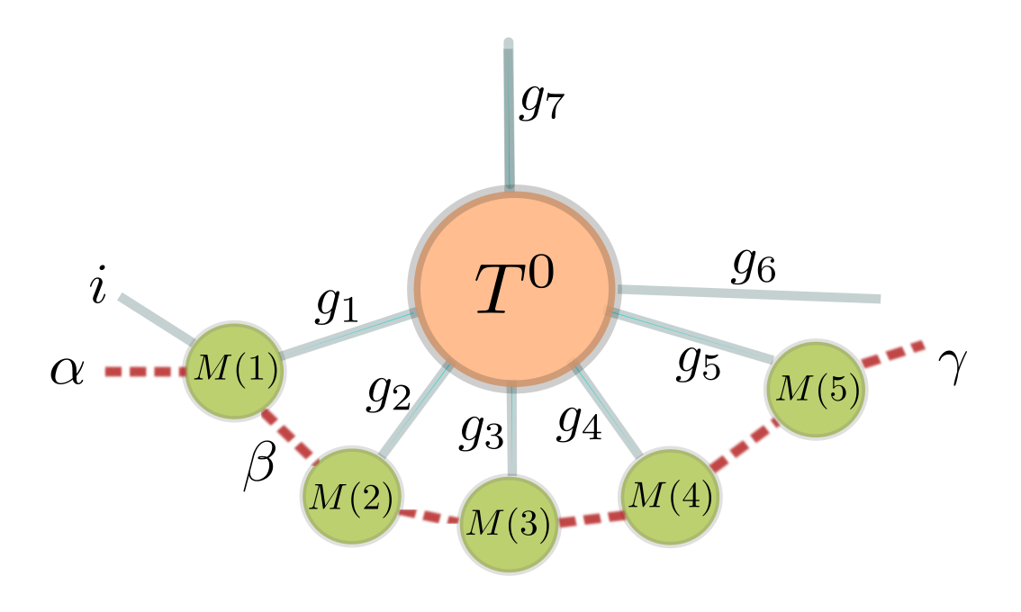
Consider the tensor at radius $r$ (labelled with $T^{0}$ in figure 4). For each string of indices $g_{1},...,g_{m}$ for which $T^{0}_{g_{1},...,g_{m}}\neq 0$, we contract the other tensors (labelled by $M(k)$ with $k\in\{1,...,m-2\}$ in figure 4). This entails multiplying a constant number of matrices. As $g_{1}$ is now fixed, the first tensor $M(1)^{i\,g_{1}}_{\alpha\beta}$ consists of four $D[r+1]\times D[r+1]$ matrices for each value of index $i$ (in practice, it is easier to view it as a $D[r]\times D[r+1]$ matrix, though the bound we would get would be a bit more convoluted). The other tensors $M(k)$ are $D[r+1]\times D[r+1]$ matrices. So, since there are $m-2$ tensors $M(k)$, the complexity of contracting them is $4(m-3)\times c_{\mathrm{mat}}D[r+1]^{n_{\mathrm{mat}}}$, where we are assuming that multiplying two $N\times N$ matrices takes at most $c_{\mathrm{mat}}N^{n_{\mathrm{mat}}}$ operations. The fastest known algorithm has $n_{\mathrm{mat}}\simeq 2.37$ [35], but typically different algorithms are used in practice with a slightly higher value of $n_{\mathrm{mat}}$. We have to do this contraction for each nonzero value of $T^{0}_{g_{1},...,g_{m}}$, which is a total of (at most) $2^{m}$ different contractions. (This is because each code tensor has at most $2^{m}$ non-zero entries.) Thus, we get a total of $2^{m+2}(m-3)c_{\mathrm{mat}}D[r+1]^{n_{\mathrm{mat}}}$ operations to do the contraction in figure 4.

However, some of the tensors at radius $r$ will actually have two legs joined to tensors at radius $r-1$ as opposed to one, which means there are only $m-3$ tensors $M(k)$ to contract, so these cases require fewer operations, i.e., $2^{m+2}(m-4)c_{\mathrm{mat}}D[r+1]^{n_{\mathrm{mat}}}$, but for the sake of simplicity, for each contraction we use the larger value.

For the final contraction with the central tensor, for each string of indices $g_{1},...,g_{m}$ for which $T(L)_{g_{1},...,g_{m}}\neq 0$, we take the trace of the product of tensors at radius two. So we multiply $m$ matrices and take the trace, which takes at most $(m-1)c_{\mathrm{mat}}D[2]^{n_{\mathrm{mat}}}+D[2]$ operations. Since we do this at most $2^{m}$ times, we get a total of $2^{m}((m-1)c_{\mathrm{mat}}D[2]^{n_{\mathrm{mat}}}+D[2])$ operations. However, this is less than the general formula $2^{m+2}(m-3)c_{\mathrm{mat}}D[r+1]^{n_{\mathrm{mat}}}$ with $r=1$, so we can use the general expression as an upper bound.

Let us denote the number of tensors at radius $r$ by $n_{\mathrm{tens}}(r)$. Then the total number of operations is bounded above by

where we defined $K=2^{m+2}(m-3)c_{\mathrm{mat}}$.

Next we use that the number of tensors at each radius increases exponentially. E.g., for the holographic code we are considering, each tensor at radius $r$ has at least five outgoing legs (to radius $r+1$), so there are at least four unique tensors at radius $r+1$ for each tensor at radius $r$. (See figure 2.) So we choose the largest $\gamma>1$ (which is at least four for our example) such that

References

- [1] J. C. Bridgeman and C. T. Chubb. Hand-waving and interpretive dance: an introductory course on tensor networks. Journal of Physics A: Mathematical and Theoretical, 50(22):223001, 2017.
- [2] S. Bravyi, M. Suchara, and A. Vargo. Efficient algorithms for maximum likelihood decoding in the surface code. Phys. Rev. A, 90:032326, 2014.
- [3] D. K. Tuckett, A. S. Darmawan, C. T. Chubb, S. Bravyi, S. D. Bartlett, and S. T. Flammia. Tailoring surface codes for highly biased noise. Phys. Rev. X, 9:041031, 2019.
- [4] D. K. Tuckett, S. D. Bartlett, and S. T. Flammia. Ultrahigh error threshold for surface codes with biased noise. Phys. Rev. Lett., 120:050505, 2018.
- [5] C. T. Chubb and S. T. Flammia. Statistical mechanical models for quantum codes with correlated noise. arXiv:1809.10704, 2018.
- [6] A. S. Darmawan and D. Poulin. Tensor-network simulations of the surface code under realistic noise. Phys. Rev. Lett., 119:040502, 2017.
- [7] A. S. Darmawan and D. Poulin. Linear-time general decoding algorithm for the surface code. Phys. Rev. E, 97:051302, 2018.
- [8] A. J. Ferris and D. Poulin. Tensor networks and quantum error correction. Phys. Rev. Lett., 113:030501, 2014.
- [9] A. J. Ferris and D. Poulin. Branching MERA codes: A natural extension of classical and quantum polar codes. In 2014 IEEE International Symposium on Information Theory, pages 1081–1085, 2014.
- [10] F. Pastawski, B. Yoshida, D. Harlow, and J. Preskill. Holographic quantum error-correcting codes: toy models for the bulk/boundary correspondence. J. High Energ. Phys., 2015:149, 2015.
- [11] J. I. Latorre and G. Sierra. Holographic codes. arXiv:1502.06618, 2015.
- [12] P. Hayden, S. Nezami, X.-L. Qi, N. Thomas, M. Walter, and Z. Yang. Holographic duality from random tensor networks. J. High Energ. Phys., 9:2016, 2016.
- [13] G. Evenbly. Hyperinvariant tensor networks and holography. Phys. Rev. Lett., 119:141602, 2017.
- [14] A. Jahn, M. Gluza, F. Pastawski, and J. Eisert. Holography and criticality in matchgate tensor networks. Science Advances, 5(8), 2019.
- [15] A. Jahn, M. Gluza, F. Pastawski, and J. Eisert. Majorana dimers and holographic quantum error-correcting codes. Phys. Rev. Research, 1:033079, 2019.
- [16] T. Kohler and T. Cubitt. Toy models of holographic duality between local Hamiltonians. J. High Energ. Phys., 17, 2019.
- [17] T. J. Osborne and D. E. Stiegemann. Dynamics for holographic codes. J. High Energ. Phys., 154, 2020.
- [18] D. Harlow. Jerusalem lectures on black holes and quantum information. Rev. Mod. Phys., 88:015002, 2016.
- [19] S. Ryu and T. Takayanagi. Holographic derivation of entanglement entropy from the anti–de Sitter space/conformal field theory correspondence. Phys. Rev. Lett., 96:181602, 2006.
- [20] R. J. Harris, N. A. McMahon, G. K. Brennen, and T. M. Stace. Calderbank-Shor-Steane holographic quantum error-correcting codes. Phys. Rev. A, 98:052301, 2018.
- [21] J. Berger and T. J. Osborne. Perfect tangles. arXiv:1804.03199, 2018.
- [22] A. Steane. Multiple-particle interference and quantum error correction. Proceedings of the Royal Society of London. Series A: Mathematical, Physical and Engineering Sciences, 452(1954):2551–2577, 1996.
- [23] R. J. Harris, E. Coupe, N. A. McMahon, G. K. Brennen, and T. M. Stace. Maximum Likelihood Decoder for Holographic Codes. arXiv:2008.10206, 2020.
- [24] H. Bombin, R. S. Andrist, M. Ohzeki, H. G. Katzgraber, and M. A. Martin-Delgado. Strong resilience of topological codes to depolarization. Phys. Rev. X, 2:021004, 2012.
- [25] D. Gottesman. Stabilizer codes and quantum error correction. PhD thesis, California Institute of Technology, 1997.
- [26] D. Gottesman. An Introduction to Quantum Error Correction and Fault-Tolerant Quantum Computation. arXiv:0904.2557, 2009.
- [27] M. A. Nielsen and I. L. Chuang. Quantum Computation and Quantum Information. Cambridge University Press, 2010.
- [28] J. Roffe. Quantum error correction: an introductory guide. Contemporary Physics, 60(3):226–245, 2019.
- [29] B. Shaw, M. M. Wilde, O. Oreshkov, I. Kremsky, and D. A. Lidar. Encoding one logical qubit into six physical qubits. Phys. Rev. A, 78:012337, 2008.
- [30] M.-H. Hsieh and F. Le Gall. NP-hardness of decoding quantum error-correction codes. Phys. Rev. A, 83:052331, 2011.
- [31] P. Iyer and D. Poulin. Hardness of decoding quantum stabilizer codes. arXiv:1310.3235, 2013.
- [32] J. Fan, Y. Li, M.-H. Hsieh, and H. Chen. On quantum tensor product codes. Quantum Information & Computation, 17:1105–1122, 2017.
- [33] M. Grassl, P. Shor, G. Smith, J. Smolin, and B. Zeng. Generalized concatenated quantum codes. Phys. Rev. A, 79:050306, 2009.
- [34] Y. Wang, B. Zeng, M. Grassl, and B. C. Sanders. Stabilizer formalism for generalized concatenated quantum codes. In 2013 IEEE International Symposium on Information Theory, pages 529–533, 2013.
- [35] F. Le Gall. Powers of tensors and fast matrix multiplication. In Proceedings of the 39th International Symposium on Symbolic and Algebraic Computation, pages 296–303, 2014.
- [36] C. Wang, J. Harrington, and J. Preskill. Confinement-Higgs transition in a disordered gauge theory and the accuracy threshold for quantum memory. Annals of Physics, 303(1):31 – 58, 2003.
Appendix A Relation of code tensors to encoding unitaries
The code tensors , defined in equation (2), can be related to any encoding unitary as follows. Consider a unitary that takes products of Pauli operators to products of Pauli operators (a Clifford unitary). This can be represented as a simple tensor , defined via